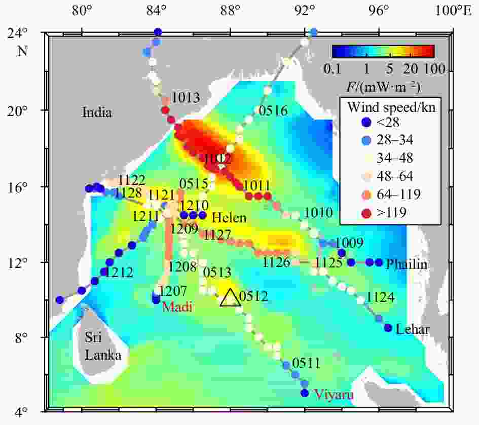
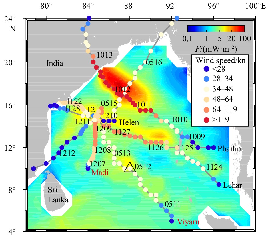
Figure  1.  Distribution of annual-mean near-inertial energy flux (colors) in the BoB in 2013. The mooring location is indicated by the black triangle. Gray solid lines and color dots give the paths and strength levels of TCs in 2013, respectively. Dates (MMDD) are marked along the tracks besides the dots. The color dots represent the maximum sustained wind speed (in knots) of the TCs. The near-inertial energy flux (F) is computed by solving the Pollard-Millard slab model using the spectral method (Alford, 2003) with National Centers for Environmental Prediction (NCEP) Climate Forecast Version 2 (CSFv2) 6-hourly wind data (Saha et al., 2014) with the mixed layer depth in the slab model set to 15 m.

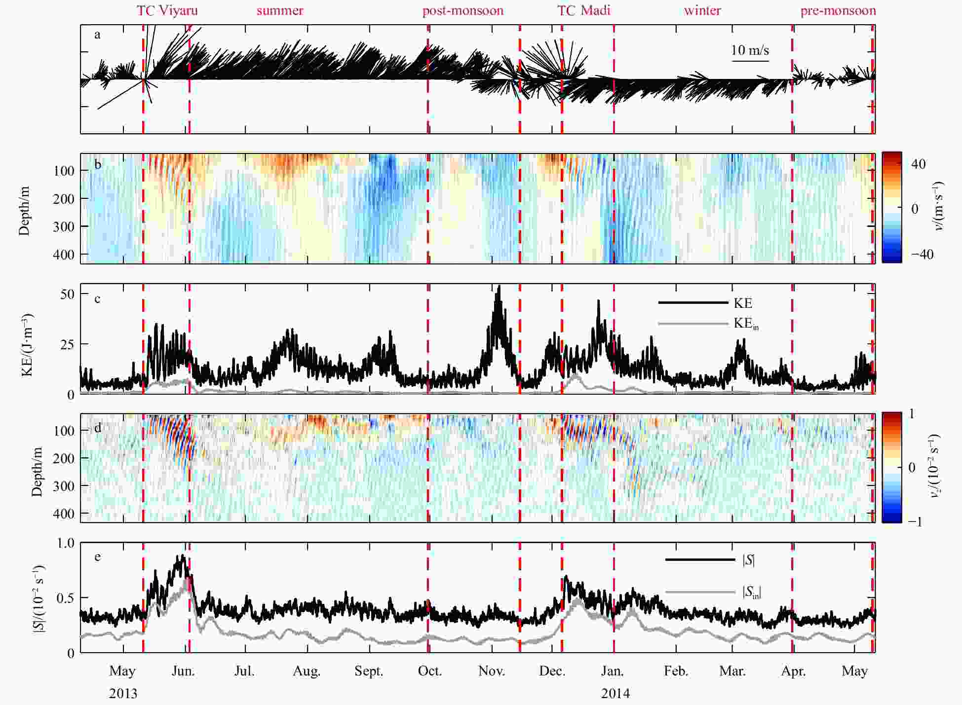
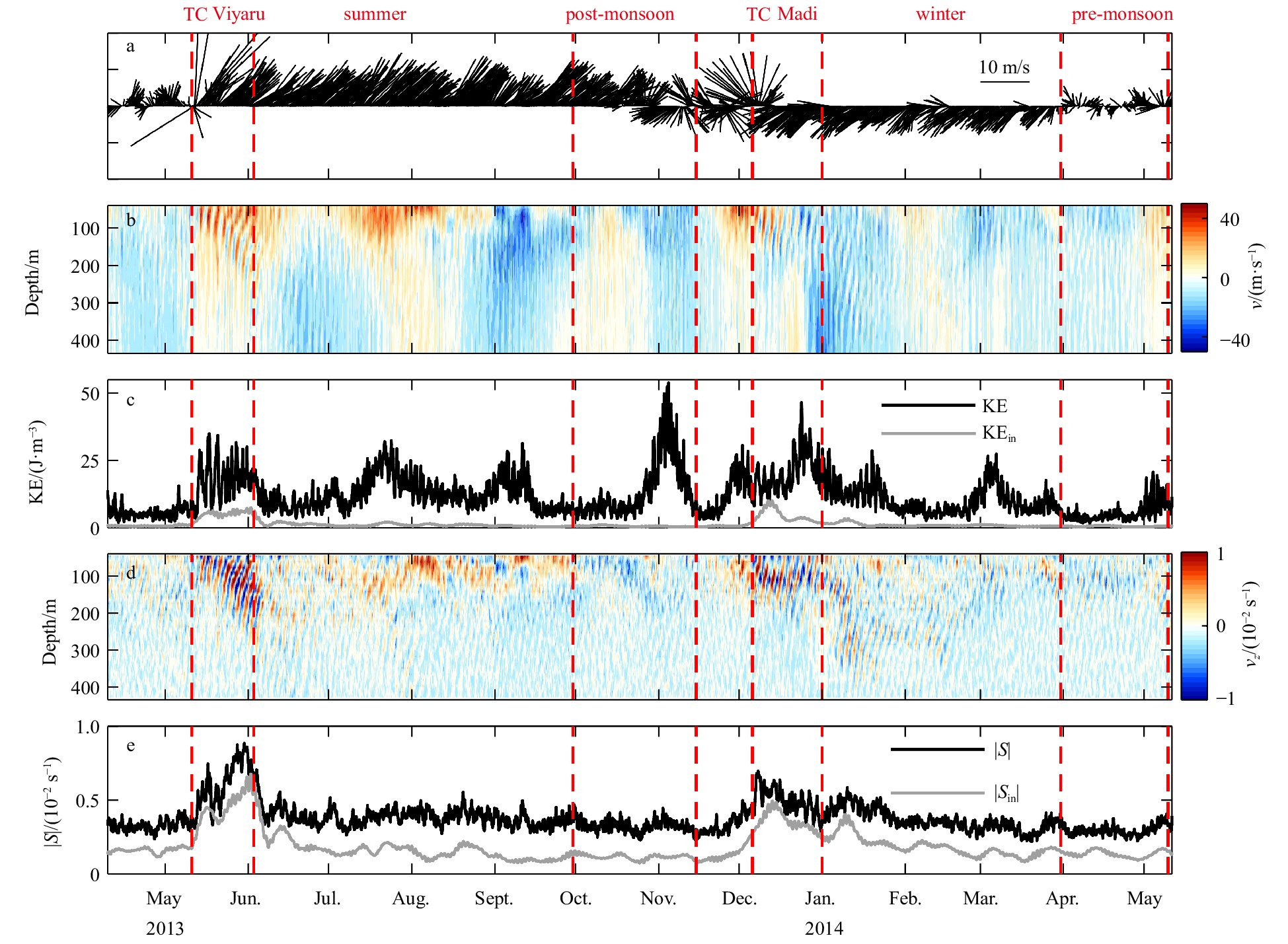
Figure  2.  Mooring observations of the velocity and shear. Surface wind acquired from the NCEP CFSv2 6-hourly winds (a), observed meridional velocity (b), vertical mean of the total and near-inertial KE (c), vertical gradient of the meridional velocity (d), and vertical mean of the magnitude of the total shear and near-inertial shear (e). The red dashed lines divide the observations into six periods: TC Viyaru (May 11–June 3, 2013), summer monsoon (June–September, 2013), post-monsoon (October–mid November, 2013), TC Madi (December 6–31, 2013), winter monsoon (January–March, 2014) and pre-monsoon (April 1–May 11, 2014).

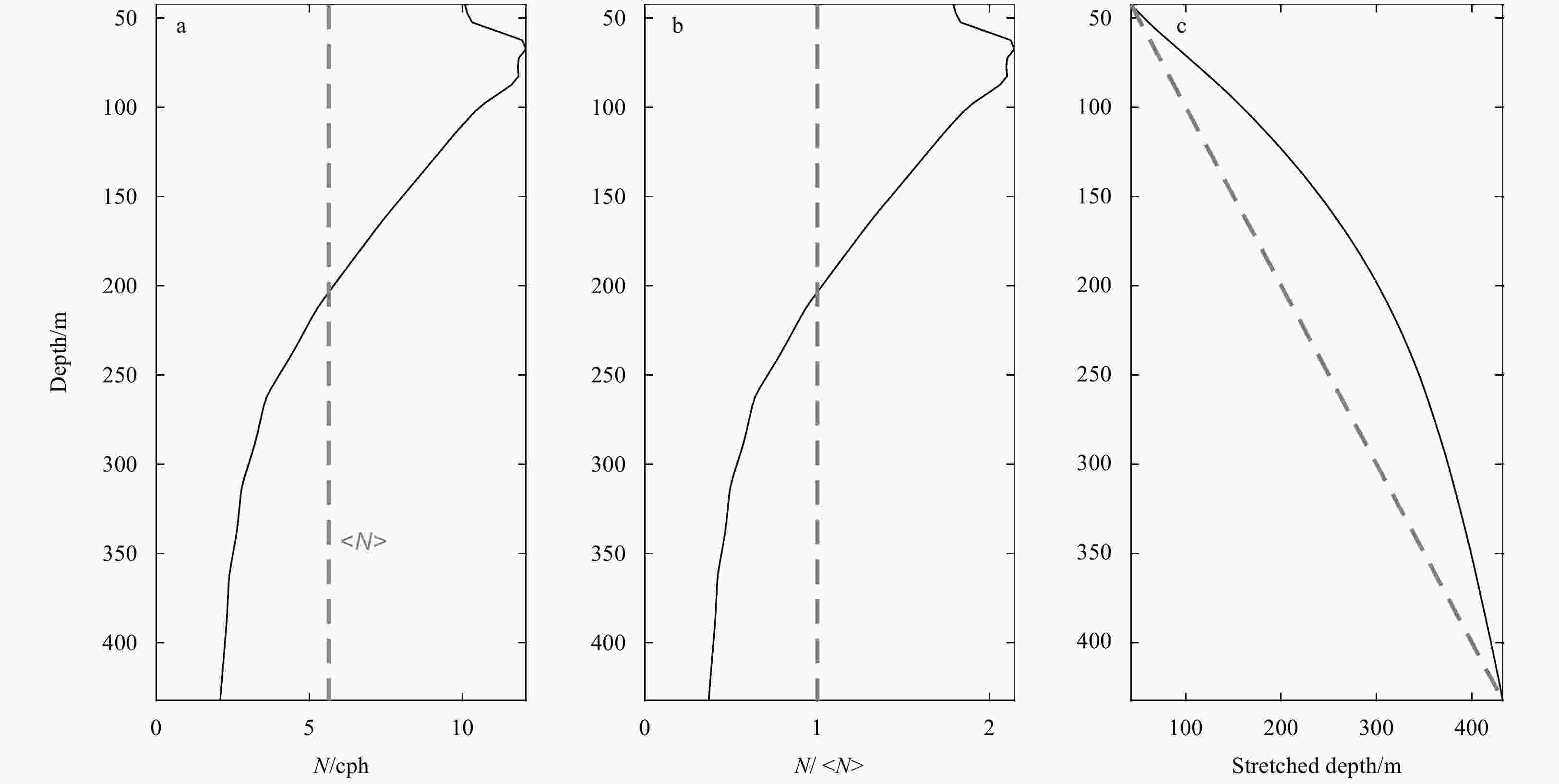
Figure  3.  Buoyancy frequency profile and the WKB-stretched depth. The annual-mean profile of buoyancy frequency from WOA2018 (a), WKB-scale factor (b), and the WKB-stretched depth versus actual depth (c).

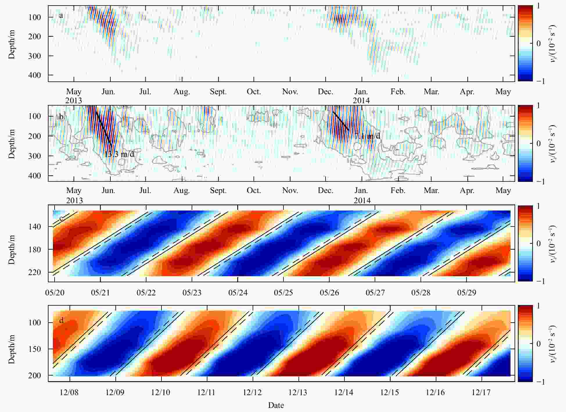
Figure  4.  Near-inertial shear and plane wave solutions. a. Bandpass filtered near-inertial meridional shear from April 9, 2013 to May 11, 2014. b. Same as a, but for the bandpass filtered near-inertial meridional shear with WKB scaling. The gray lines give the areas where vector correlation coefficients between the total shear and the near-inertial shear exceeds 0.7. The black lines indicate the rays of NIWs propagating downward, and the group velocity is shown along the side. c. Snapshot of the TC Viyaru case between 112 m and 227 m (stretched depth). The time ticks are in format mm/dd. d. Same as c, but for the TC Madi case between 77 m and 202 m (stretched depth). The solid and dashed lines represent contours of 0.1 and –0.1 of the plane wave solutions, respectively.

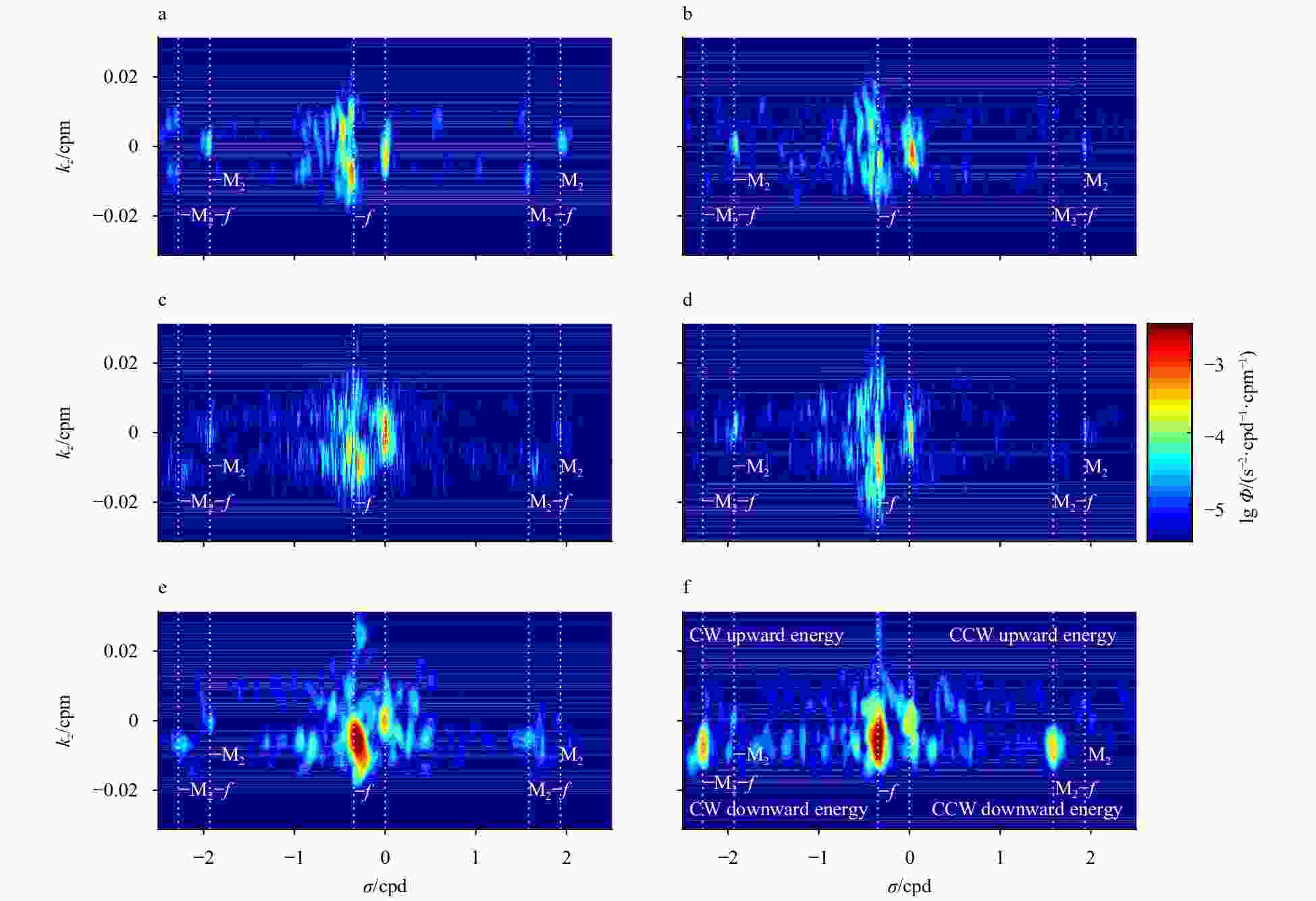
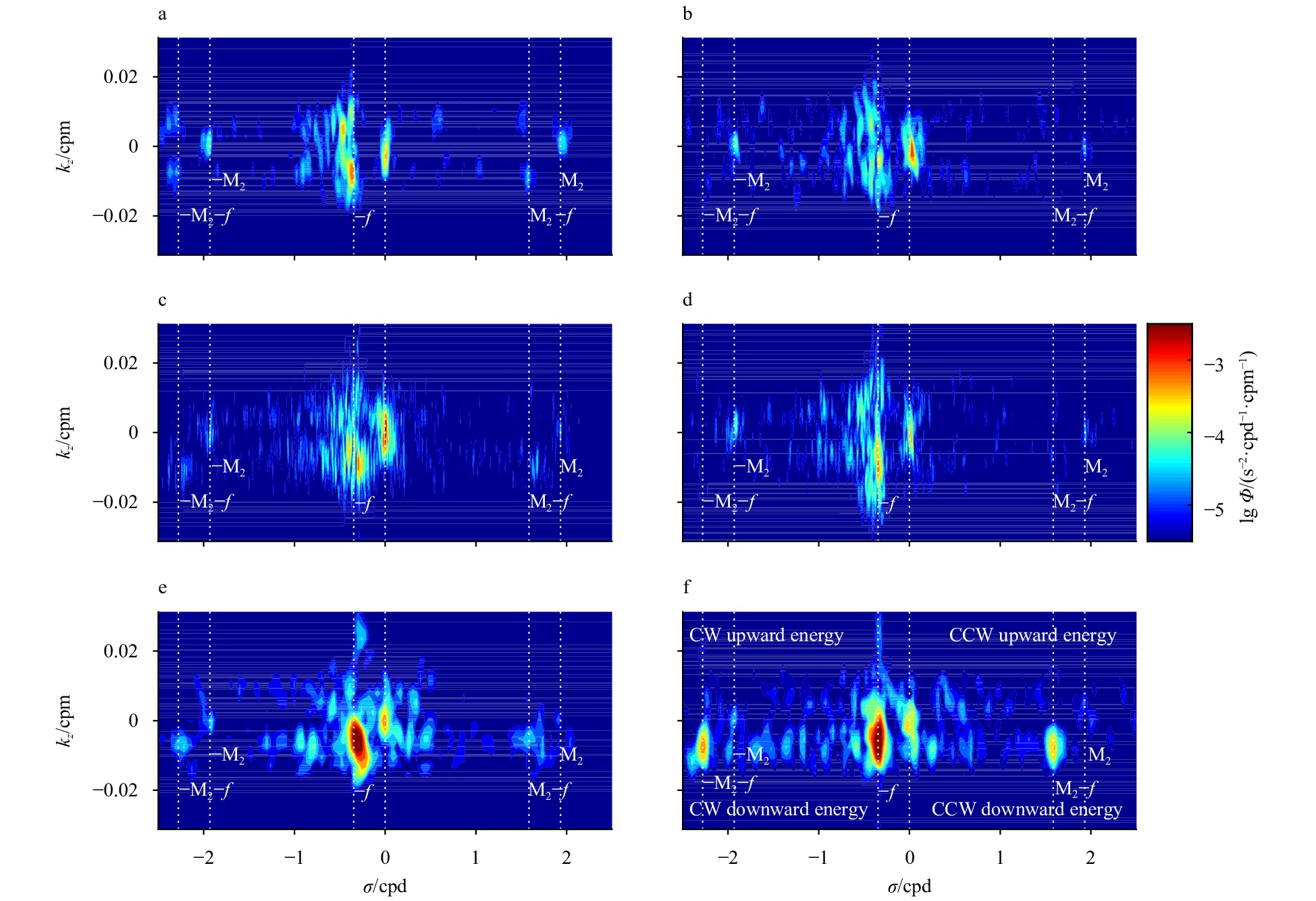
Figure  5.  Wavenumber-frequency spectra for different periods. a. Pre-monsoon, b. post-monsoon, c. summer monsoon, d. winter monsoon, e. TC Viyaru, and f. TC Madi. The division of the periods is the same as that presented in Fig. 2. The gray dashed lines represent different frequencies, and the corresponding frequencies are shown. The abscissa is wave frequency, σ, in cycle per day (cpd), and the ordinate is vertical wavenumber, k_z, in cycle per meter (cpm).

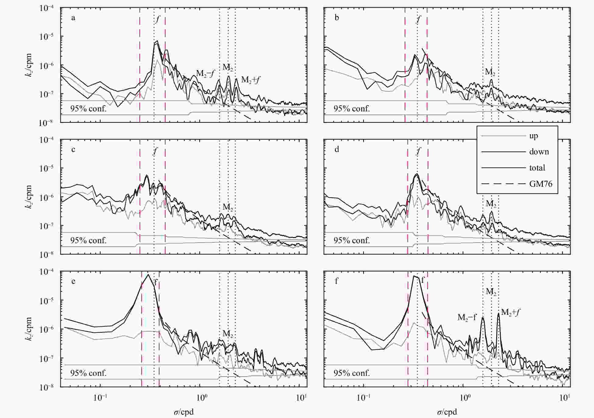
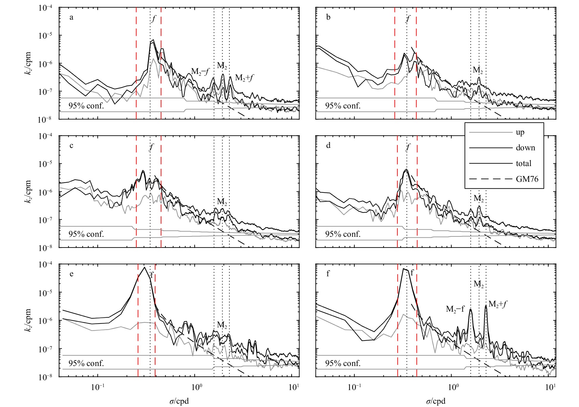
Figure  6.  Rotary frequency spectra for different periods. a. Pre-monsoon, b. post-monsoon, c. summer monsoon, d. winter monsoon, e. TC Viyaru, and f. TC Madi. The red dashed lines indicate the near-inertial frequency bands determined by the ratio of clockwise and counterclockwise components exceeding 3 (see the text). Horizontal gray lines give the confidence intervals of the spectra, with degrees of freedom varying with increasing frequency, σ, in cycle per day (cpd), and the ordinate is vertical wavenumber, k_z, in cycle per meter (cpm).

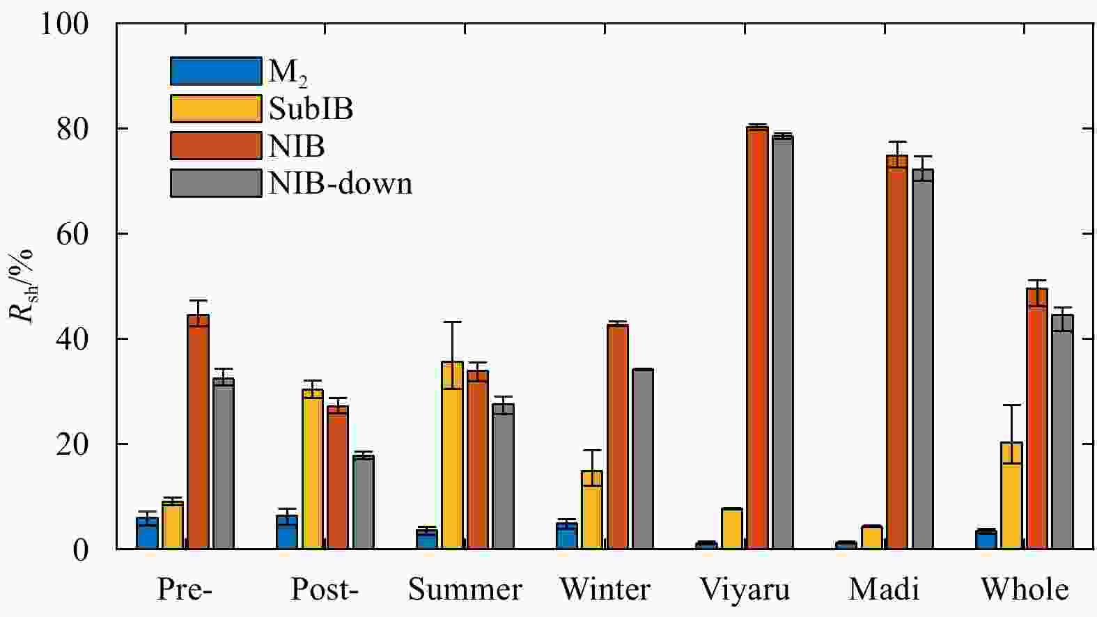
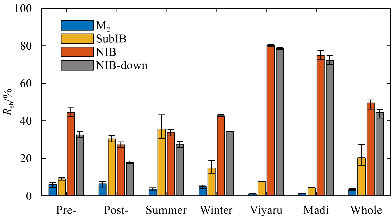
Figure  7.  Histogram of the percentage of shear variances in total variances. The error bars were estimated by the corresponding 95% confidence intervals given in Fig. 6.

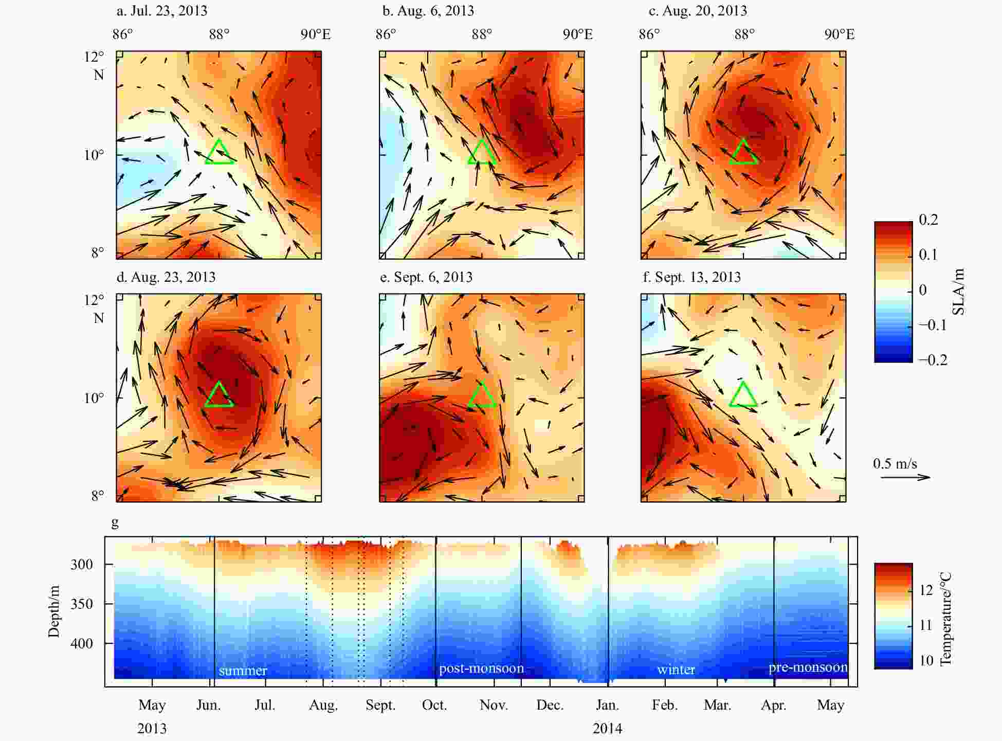
Figure  8.  Sea surface anomaly (SLA; a–f) and mooring temperature observations (g) . SLA and surface geostrophic currents correspond to the dates indicated by the dashed lines in g. The green triangle represents the location of the mooring. Contours of temperature data are beneath 280 m in g. The black solid lines in g give four of the six periods indicated by the red dashed lines in Fig. 2.

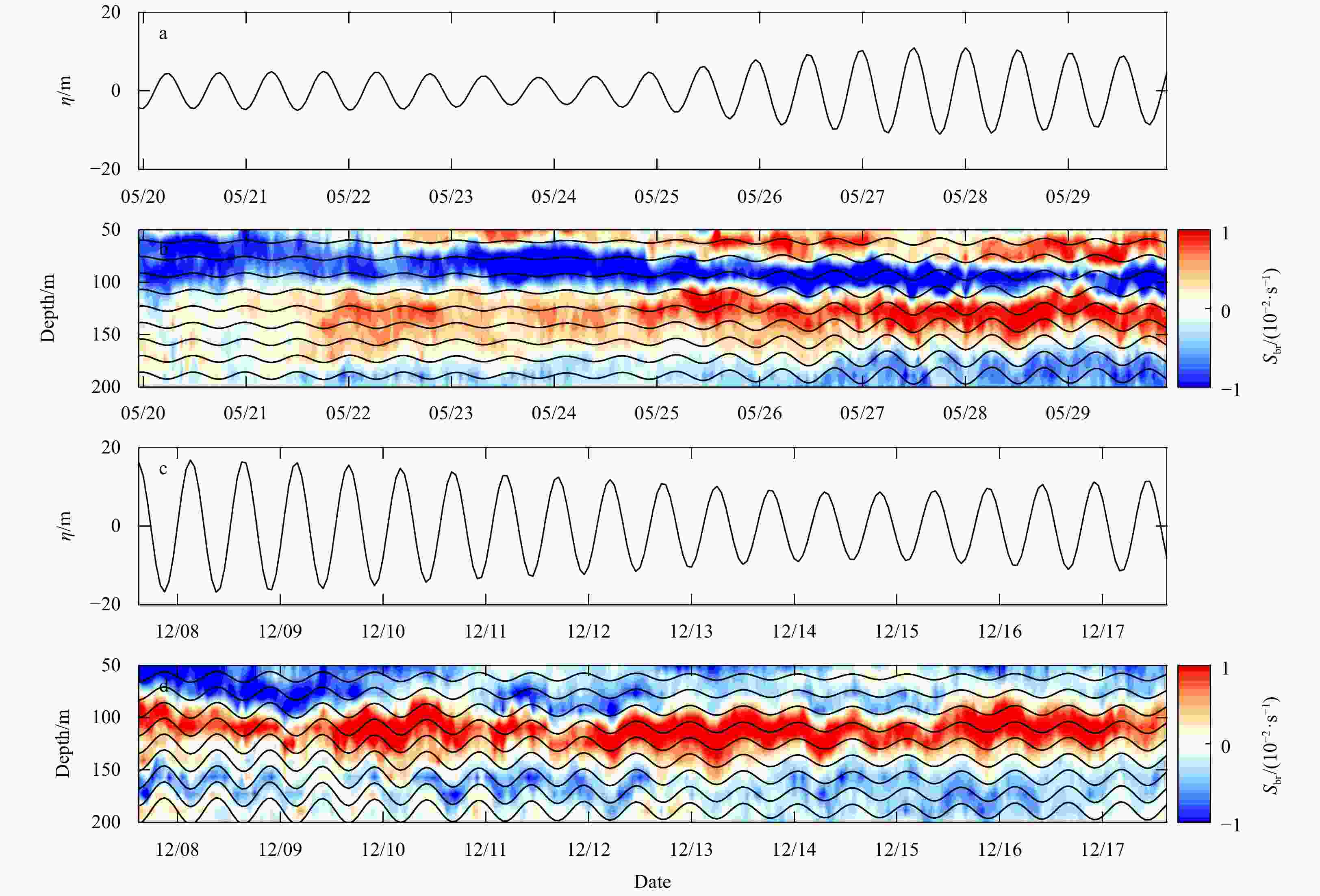
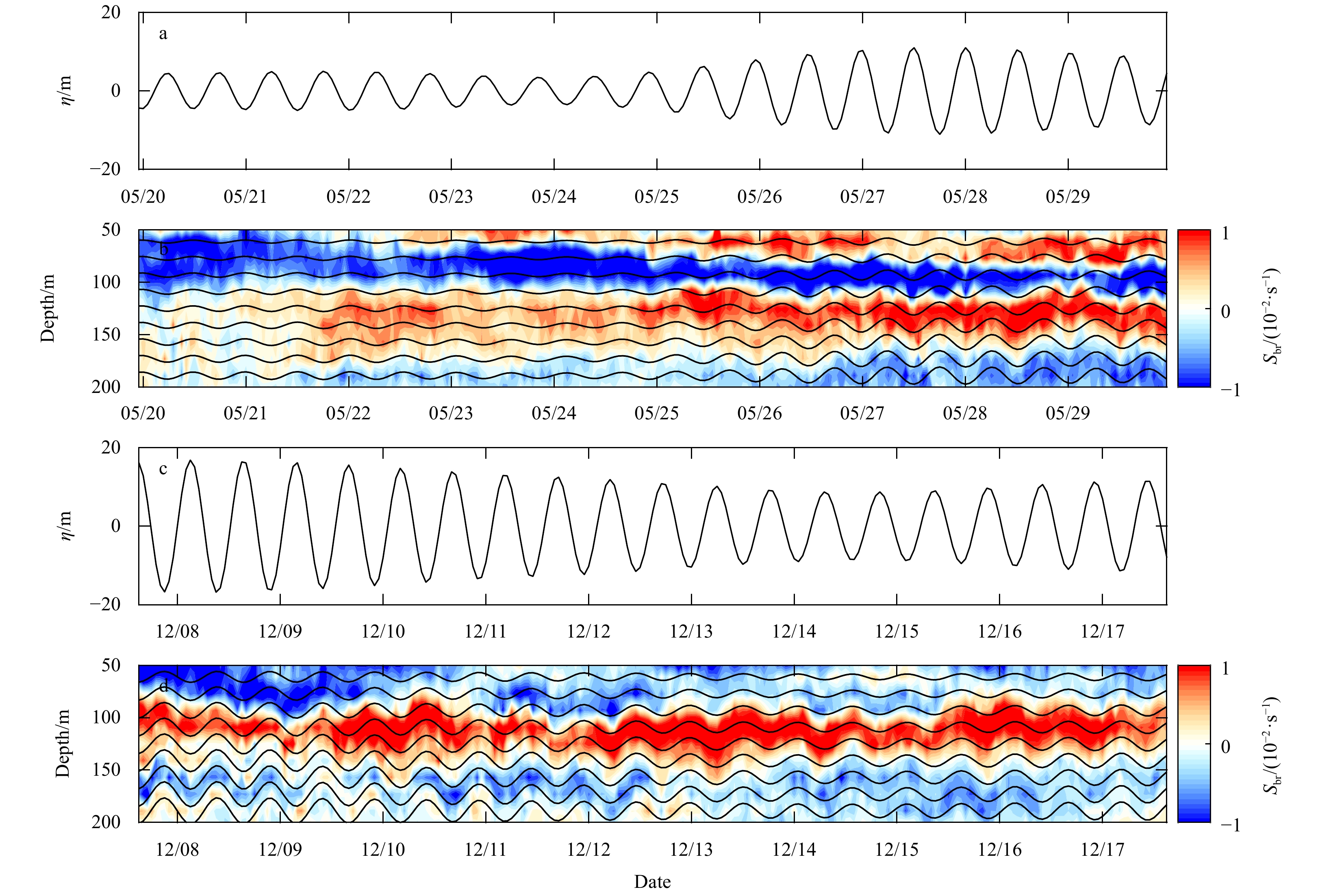
Figure  9.  Backrotated shear and internal tide displacements. M₂ tidal components of the isotherm of 11°C for TC Viyaru (May 2013) (a) and TC Madi (December 2013) (b). The corresponding real part of the backrotated shear (S_br) between 50 m and 200 m with internal tide displacements superimposed (black solid lines) (b, d).