

Mapping wind by the first-order Bragg scattering of broad-beam high-frequency radar
-
Abstract: Mapping wind with high-frequency (HF) radar is still a challenge. The existing second-order spectrum based wind speed extraction method has the problems of short detection distances and low angular resolution for broad-beam HF radar. To solve these problems, we turn to the first-order Bragg spectrum power and propose a space recursion method to map surface wind. One month of radar and buoy data are processed to build a wind spreading function model and a first-order spectrum power model describing the relationship between the maximum of first-order spectrum power and wind speed in different sea states. Based on the theoretical propagation attenuation model, the propagation attenuation is calculated approximately by the wind speed in the previous range cell to compensate for the first-order spectrum in the current range-azimuth cell. By using the compensated first-order spectrum, the final wind speed is extracted in each cell. The first-order spectrum and wind spreading function models are tested using one month of buoy data, which illustrates the applicability of the two models. The final wind vector map demonstrates the potential of the method.
-
Key words:
- high-frequency radar /
- first-order Bragg peak /
- broad-beam /
- wind field /
- wind speed
-
Figure 2. Attenuation of first-order spectrum power (FSP) result from the wind spreading function (WSF) with different
$s$ .
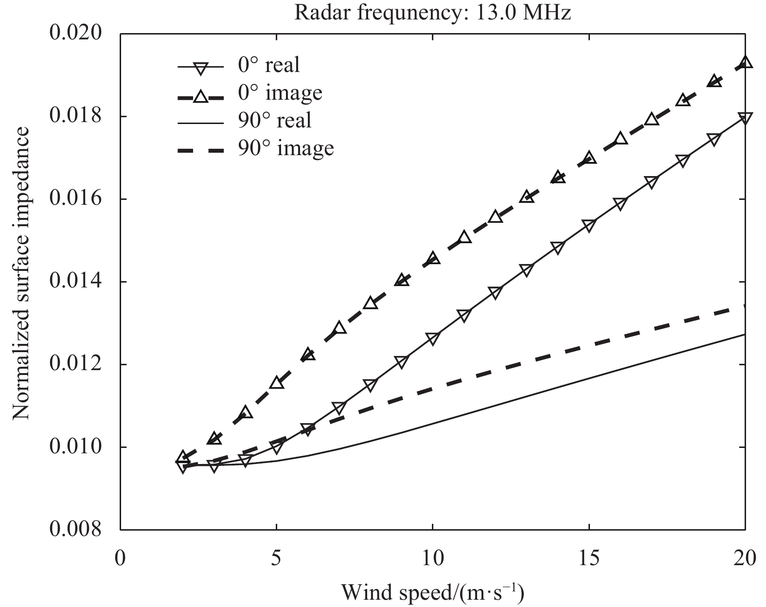
Figure 3. Normalized surface impedance for 13 MHz radar wave under different wind speed,
$ {0}^{\circ } $ represents radial wind and$ {90}^{\circ } $ represents cross wind. The solid and broken lines represent the real and imaginary parts of the impedance, respectively.
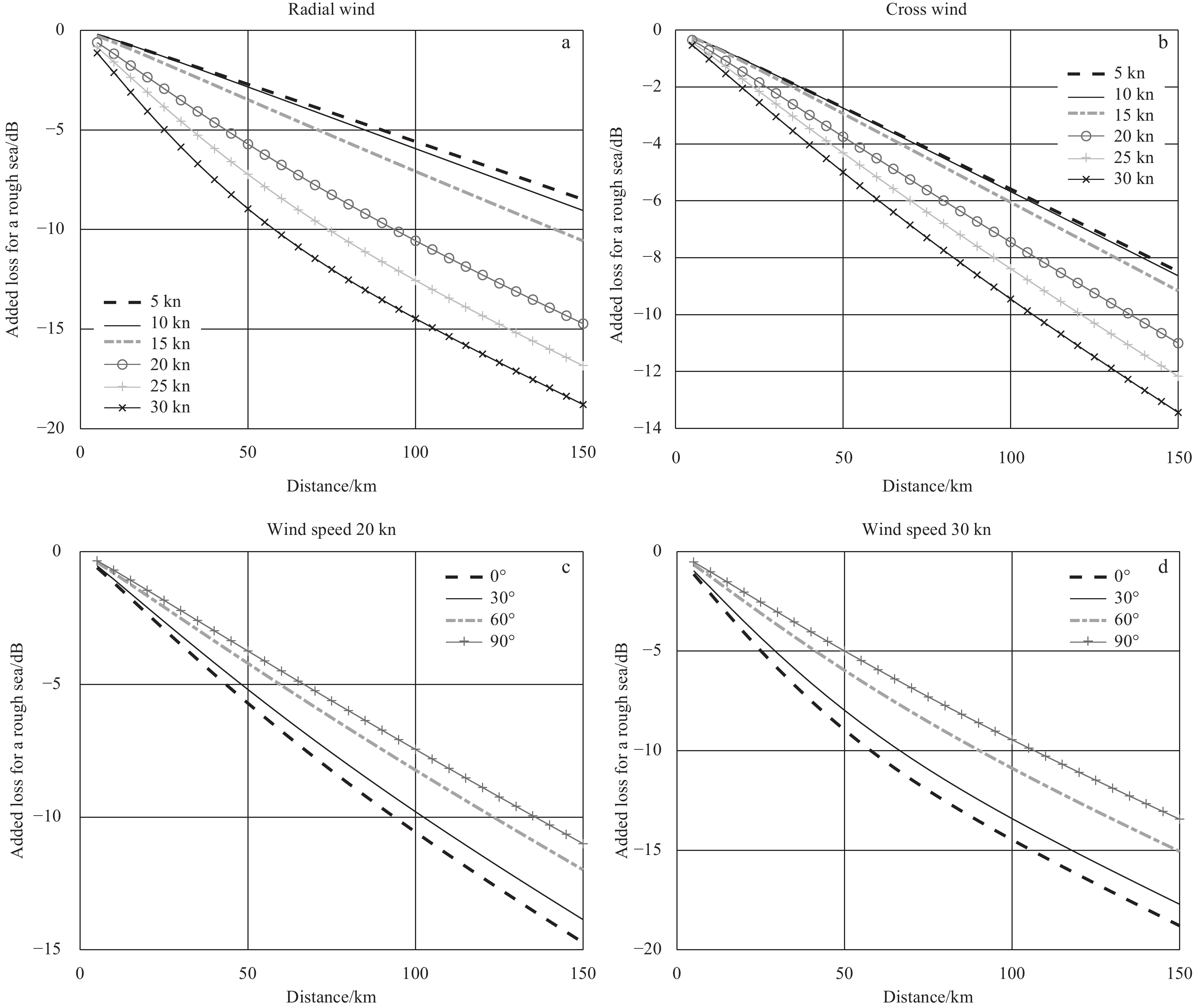
Figure 4. Added loss for a rough sea under different winds. a. Under radial wind; b. under cross wind; c. under 20 kn wind speed; and d. under 30 kn wind speed.
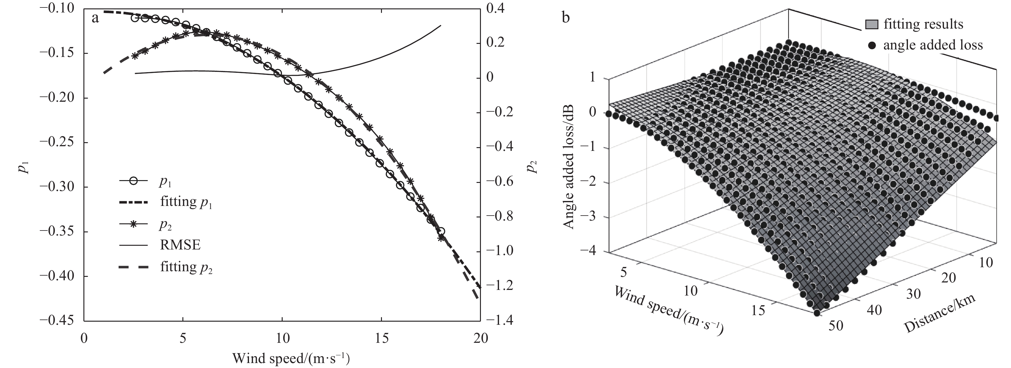
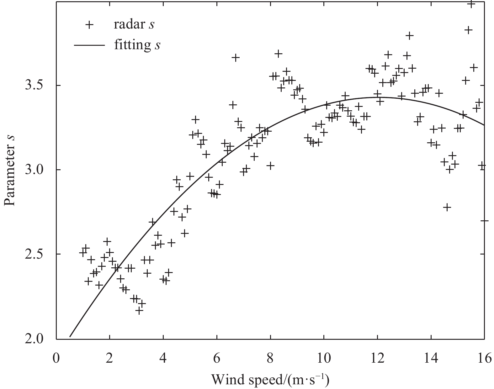
Figure 5. Fitting of the parameters under different radial winds (a), and discrepancy loss between radial wind and cross wind under different wind speeds (b).

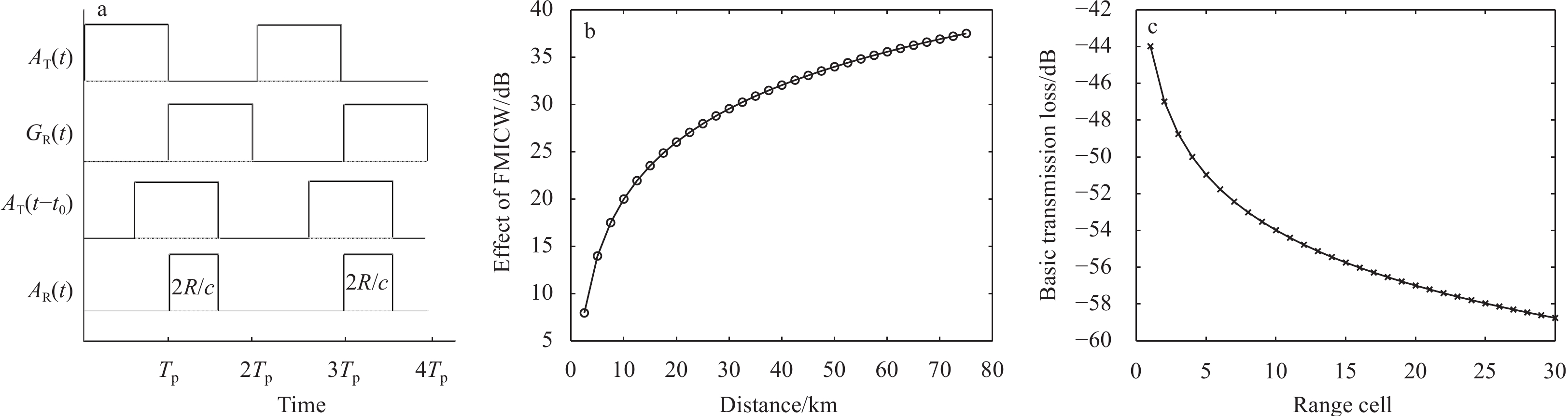
Figure 6. Modulation process of a gate signal to a receiving signal (a), effect of the gate signal on the radar echo power (b), and basic transmission loss for a monostatic 13 MHz OSMAR radar (c). Each range cell is
$ 2.5 $ km. In a, AT is the transmit pulse, GR is the receive pulse, t0 is the delay corresponding to distance R, AR is the effective receive pulse for distance R, and Tp is the sweep period.
Figure 7. Total transmission loss for a rough sea for the monostatic 13 MHz OSMSAR radar. a. Under radial wind; and b. under cross wind.
Figure 9. Map of the HF radar deployed on the Fujian coast of the Taiwan Strait. Radar station is marked by the star named XIAN, and the three buoys are marked by dots.
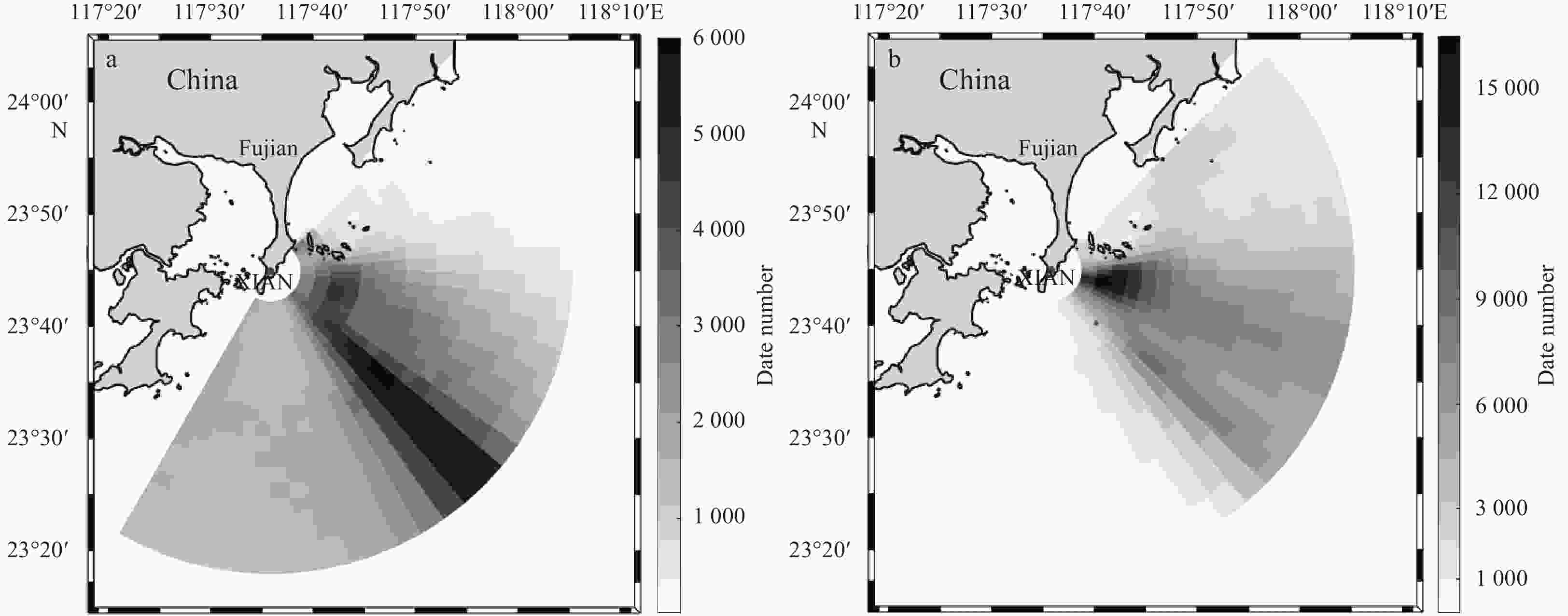
Figure 11. Number of DOA solutions in each measurement bin, where the total number of measurements is 6 202. a. For positive FSPs; and b. for negative FSPs.

Figure 12. The maximum FSPs versus wind speeds for different range cells (a); and the maximum FSP loss (relative to the maximum FSP in range cell
$ 2 $ ) versus range cells under different wind speeds (b). Each range cell is$ 2.5 $ km.
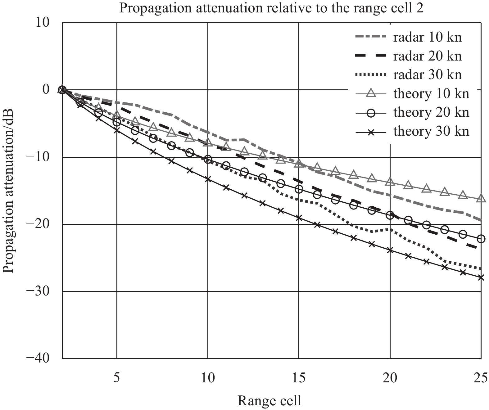
Figure 13. Comparison of the theoretical and the radar extracted propagation attenuation relative to the range cell 2 with different radial wind.
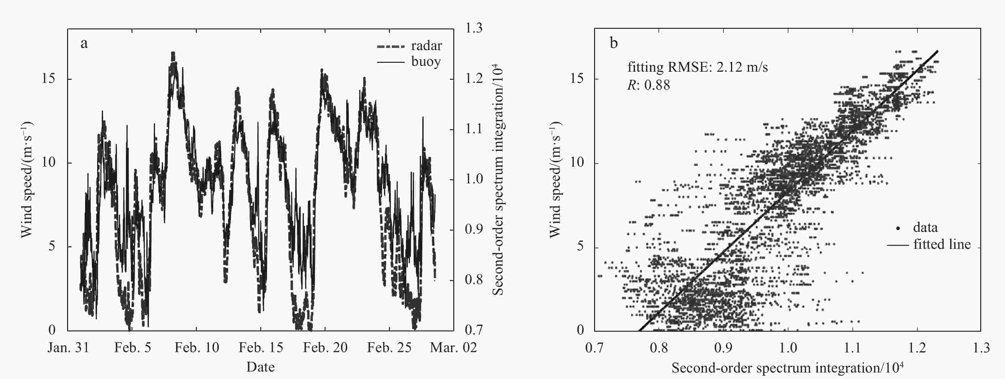
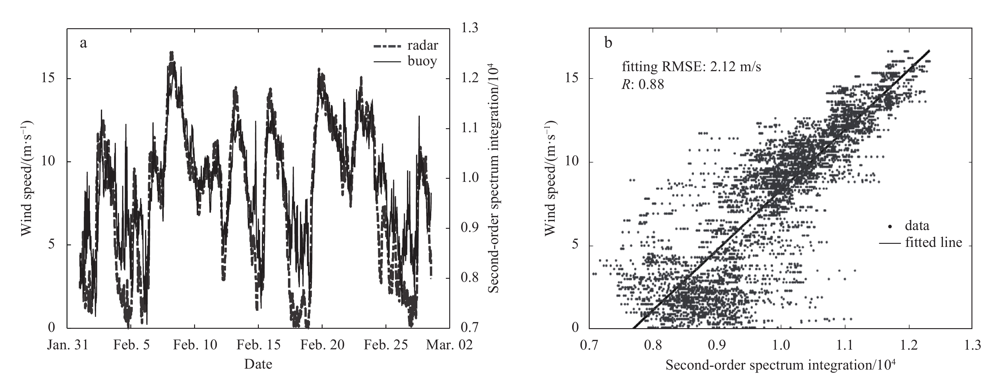
Figure 15. Wind speed and the second-order integration versus time (a); scatter plot and linear fitting result (b).

Figure 16. Wind speed and the maximum first-order peak versus time (a); and scatter plot and fitting result (b).

Figure 17. Buoy wind speed versus the second-order integration (a); and buoy wind speed versus the radar wind speed from the second-order model (b).
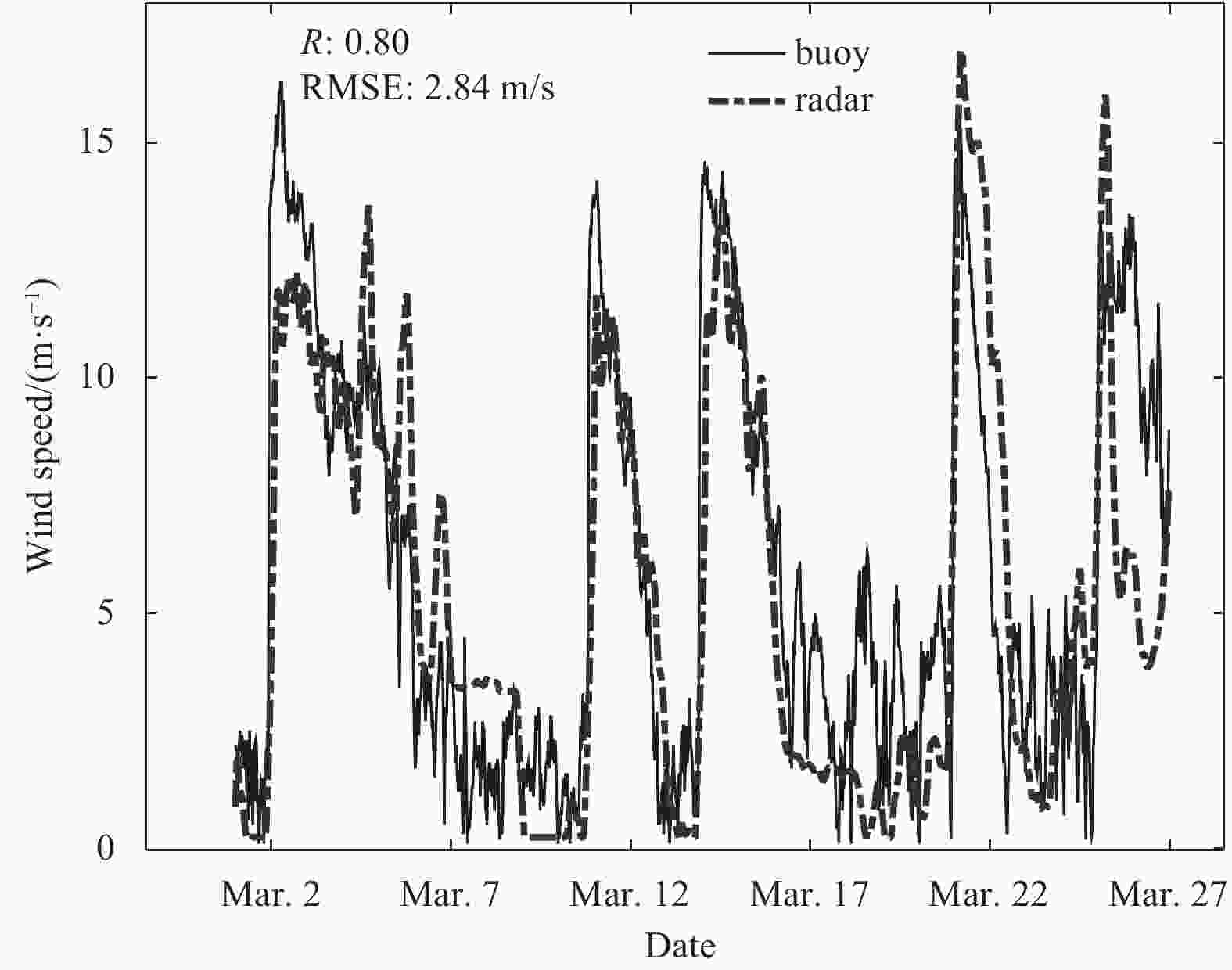
Figure 18. Comparison of the wind speed and the radar wind speed from the first-order model.

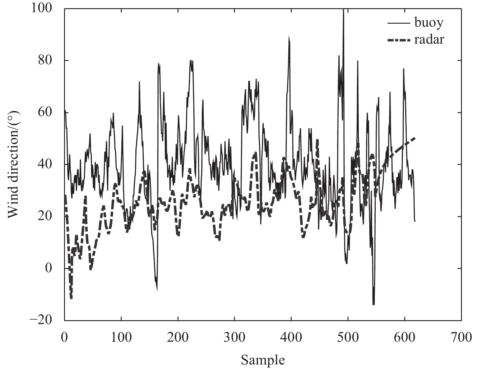
Figure 19. Sample comparisons of the in-situ measured and estimated wind direction at Buoy A in March. Note the sample numbers do not represent a time series but are individual, independent estimates of half an hour time period with wind speed above
$ 6.5 $ m/s.Table 1. Radar parameters of the OSMAR-S
Parameters Value and setting Center frequency/MHz 13 Bandwidth/kHz 60 Transmit antenna monopole Receive antenna cross-loop/monopole Sweep period/s 0.38 Average power/W 100 Range resolution/km 2.5 Coherent integration time/min 6.5 Normal direction/(°) 100 Transmitted waveform FMICW pulses Technique of azimuthal resolution direction finding  下载: 导出CSV
-
[1] Adams J E, Carroll J C, Costa E A, et al. 1984. Measurements and Predictions of HF Ground Wave Radio Propagation Over Irregular, Inhomogeneous Terrain. Boulder, CO, USA: NTIA Report, 84–151 [2] Apaydin G, Sevgi L. 2010. A novel split-step parabolic-equation package for surface-wave propagation prediction along multiple mixed irregular-terrain paths. IEEE Antennas and Propagation Magazine, 52(4): 90–97. doi: 10.1109/MAP.2010.5638238 [3] Apel J R. 1994. An improved model of the ocean surface wave vector spectrum and its effects on radar backscatter. Journal of Geophysical Research: Oceans, 99(C8): 16269–16291. doi: 10.1029/94JC00846 [4] Barrick D. 1972a. First-order theory and analysis of MF/HF/VHF Scatter from the Sea. IEEE Transactions on Antennas and Propagation, 20(1): 2–10. doi: 10.1109/TAP.1972.1140123 [5] Barrick D. 1972b. Remote sensing of sea state by radar. In: Ocean 72-IEEE International Conference on Engineering in the Ocean Environment, Newport, RI, USA: IEEE, 186–192. [6] Barrick D E. 1971. Theory of HF and VHF propagation across the rough sea, 2, Application to HF and VHF propagation above the sea. Radio Science, 6(5): 527–533. doi: 10.1029/RS006i005p00527 [7] Barrick D E. 1977. Extraction of wave parameters from measured HF radar sea-echo Doppler spectra. Radio Science, 12(3): 415–424. doi: 10.1029/RS012i003p00415 [8] Barrick D E, Headrick J M, Bogle R W, et al. 1974. Sea backscatter at HF: interpretation and utilization of the echo. Proceedings of the IEEE, 62(6): 673–680. doi: 10.1109/PROC.1974.9507 [9] Carvalho D, Rocha A, Gómez-Gesteira M, et al. 2014. Comparison of reanalyzed, analyzed, satellite-retrieved and NWP modelled winds with buoy data along the Iberian Peninsula coast. Remote Sensing of Environment, 152: 480–492. doi: 10.1016/j.rse.2014.07.017 [10] Dexter P E, Theodoridis S. 1982. Surface wind speed extraction from HF sky wave radar Doppler spectra. Radio Science, 17(3): 643–652. doi: 10.1029/RS017i003p00643 [11] Fernandez D M, Graber H C, Paduan J D, et al. 1997. Mapping wind directions with HF radar. Oceanography, 10(2): 93–95 [12] Forget P, Broche P, De Maistre J C. 1982. Attenuation with distance and wind speed of HF surface waves over the ocean. Radio Science, 17(3): 599–610. doi: 10.1029/RS017i003p00599 [13] Green D, Gill E, Huang Weimin. 2009. An inversion method for extraction of wind speed from high-frequency ground-wave radar oceanic backscatter. IEEE Transactions on Geoscience and Remote Sensing, 47(10): 3338–3346. doi: 10.1109/TGRS.2009.2022944 [14] Hasselmann D E, Dunckel M, Ewing J A. 1980. Directional wave spectra observed during jonswap 1973. Journal of Physical Oceanography, 10(8): 1264–1280. doi: 10.1175/1520-0485(1980)010<1264:DWSODJ>2.0.CO;2 [15] Heron M L. 2015. Comparisons of different HF ocean surface-wave radar technologies. In: 2015 IEEE/OES Eleveth Current, Waves and Turbulence Measurement (CWTM). St Petersburg, FL, USA: IEEE, 1–4 [16] Heron M L, Rose R J. 1986. On the application of HF ocean radar to the observation of temporal and spatial changes in wind direction. IEEE Journal of Oceanic Engineering, 11(2): 210–218. doi: 10.1109/JOE.1986.1145173 [17] Hill D A, Wait J R. 1980. Ground wave attenuation function for a spherical earth with arbitrary surface impedance. Radio Science, 15(3): 637–643. doi: 10.1029/RS015i003p00637 [18] Huang Weimin, Gill E W, Wu Shicai, et al. 2004. Measuring surface wind direction by monostatic HF ground-wave radar at the Eastern China Sea. IEEE Journal of Oceanic Engineering, 29(4): 1032–1037. doi: 10.1109/JOE.2004.834175 [19] Huang Weimin, Wu Shicai, Gill E, et al. 2002. HF radar wave and wind measurement over the Eastern China Sea. IEEE Transactions on Geoscience and Remote Sensing, 40(9): 1950–1955. doi: 10.1109/TGRS.2002.803718 [20] Khan R H, Mitchell D K. 1991. Waveform analysis for high-frequency FMICW radar. Radar and Signal Processing IEE Proceedings F, 138(5): 411–419. doi: 10.1049/ip-f-2.1991.0054 [21] Kirincich A. 2016. Remote sensing of the surface wind field over the coastal ocean via direct calibration of HF radar backscatter power. Journal of Atmospheric and Oceanic Technology, 33(7): 1377–1392. doi: 10.1175/JTECH-D-15-0242.1 [22] Lai Yeping, Zhou Hao, Wen Biyang. 2017a. Surface current characteristics in the Taiwan Strait observed by high-frequency radars. IEEE Journal of Oceanic Engineering, 42(2): 449–457. doi: 10.1109/JOE.2016.2572818 [23] Lai Yeping, Zhou Hao, Yang Jing, et al. 2017b. Submesoscale eddies in the Taiwan Strait observed by high-frequency radars: detection algorithms and eddy properties. Journal of Atmospheric and Oceanic Technology, 34(4): 939–953. doi: 10.1175/JTECH-D-16-0160.1 [24] Maresca J W, Barnum J R. 1982. Estimating wind speed from HF skywave radar sea backscatter. IEEE Transactions on Antennas and Propagation, 30(5): 846–852. doi: 10.1109/TAP.1982.1142887 [25] Pierson W J Jr, Moskowitz L. 1964. A proposed spectral form for fully developed wind seas based on the similarity theory of S. A. kitaigorodskii. Journal of Geophysical Research, 69(24): 5181–5190. doi: 10.1029/JZ069i024p05181 [26] Schmidt R. 1986. Multiple emitter location and signal parameter estimation. IEEE Transactions on Antennas and Propagation, 34(3): 276–280. doi: 10.1109/TAP.1986.1143830 [27] Shen Wei, Gurgel K W, Voulgaris G, et al. 2012. Wind-speed inversion from HF radar first-order backscatter signal. Ocean Dynamics, 62(1): 105–121. doi: 10.1007/s10236-011-0465-9 [28] Stewart R H, Barnum J R. 1975. Radio measurements of oceanic winds at long ranges: An evaluation. Radio Science, 10(10): 853–857. doi: 10.1029/RS010i010p00853 [29] Wyatt L R. 2018. A comparison of scatterometer and HF radar wind direction measurements. Journal of Operational Oceanography, 11(1): 54–63. doi: 10.1080/1755876X.2018.1443625 [30] Wyatt L R, Green J J, Middleditch A, et al. 2006. Operational wave, current, and wind measurements with the pisces HF radar. IEEE Journal of Oceanic Engineering, 31(4): 819–834. doi: 10.1109/JOE.2006.888378 [31] Zeng Yuming, Zhou Hao, Roarty H, et al. 2016. Wind speed inversion in high frequency radar based on neural network. International Journal of Antennas and Propagation, 2016: 2706521 [32] Zhang Lei, Shi Hanqing, Yu Hong, et al. 2016. WindSat satellite comparisons with nearshore buoy wind data near the U. S. west and east coasts. Acta Oceanologica Sinica, 35(7): 50–58. doi: 10.1007/s13131-016-0905-y [33] Zhou Hao, Roarty H, Wen Biyang. 2015. Wave height measurement in the Taiwan Strait with a portable high frequency surface wave radar. Acta Oceanologica Sinica, 34(1): 73–78. doi: 10.1007/s13131-015-0599-6 [34] Zhou Hao, Wang Caijun, Yang Jing, et al. 2017. Wind and current dependence of the first-order bragg scattering power in high-frequency radar sea echoes. IEEE Geoscience and Remote Sensing Letters, 14(12): 2428–2432. doi: 10.1109/LGRS.2017.2768060 [35] Zhou Hao, Wen Biyang. 2015. Wave height extraction from the first-order Bragg peaks in high-frequency radars. IEEE Geoscience and Remote Sensing Letters, 12(11): 2296–2300. doi: 10.1109/LGRS.2015.2472976 -


 点击查看大图

计量
- 文章访问数: 510
- HTML全文浏览量: 144
- PDF下载量: 24
- 被引次数: 0