

Response of the mixed layer depth and subduction rate in the subtropical Northeast Pacific to global warming
-
Abstract: The response of the mixed layer depth (MLD) and subduction rate in the subtropical Northeast Pacific to global warming is investigated based on 9 CMIP5 models. Compared with the present climate in the 9 models, the response of the MLD in the subtropical Northeast Pacific to the increased radiation forcing is spatially non-uniform, with the maximum shoaling about 50 m in the ensemble mean result. The inter-model differences of MLD change are non-negligible, which depend on the various dominated mechanisms. On the north of the MLD front, MLD shallows largely and is influenced by Ekman pumping, heat flux, and upper-ocean cold advection changes. On the south of the MLD front, MLD changes a little in the warmer climate, which is mainly due to the upper-ocean warm advection change. As a result, the MLD front intensity weakens obviously from 0.24 m/km to 0.15 m/km (about 33.9%) in the ensemble mean, not only due to the maximum of MLD shoaling but also dependent on the MLD non-uniform spatial variability. The spatially non-uniform decrease of the subduction rate is primarily dominated by the lateral induction reduction (about 85% in ensemble mean) due to the significant weakening of the MLD front. This research indicates that the ocean advection change impacts the MLD spatially non-uniform change greatly, and then plays an important role in the response of the MLD front and the subduction process to global warming.
-
Key words:
- mixed layer depth /
- mixed layer depth front /
- subduction /
- ocean advection /
- non-uniform
-
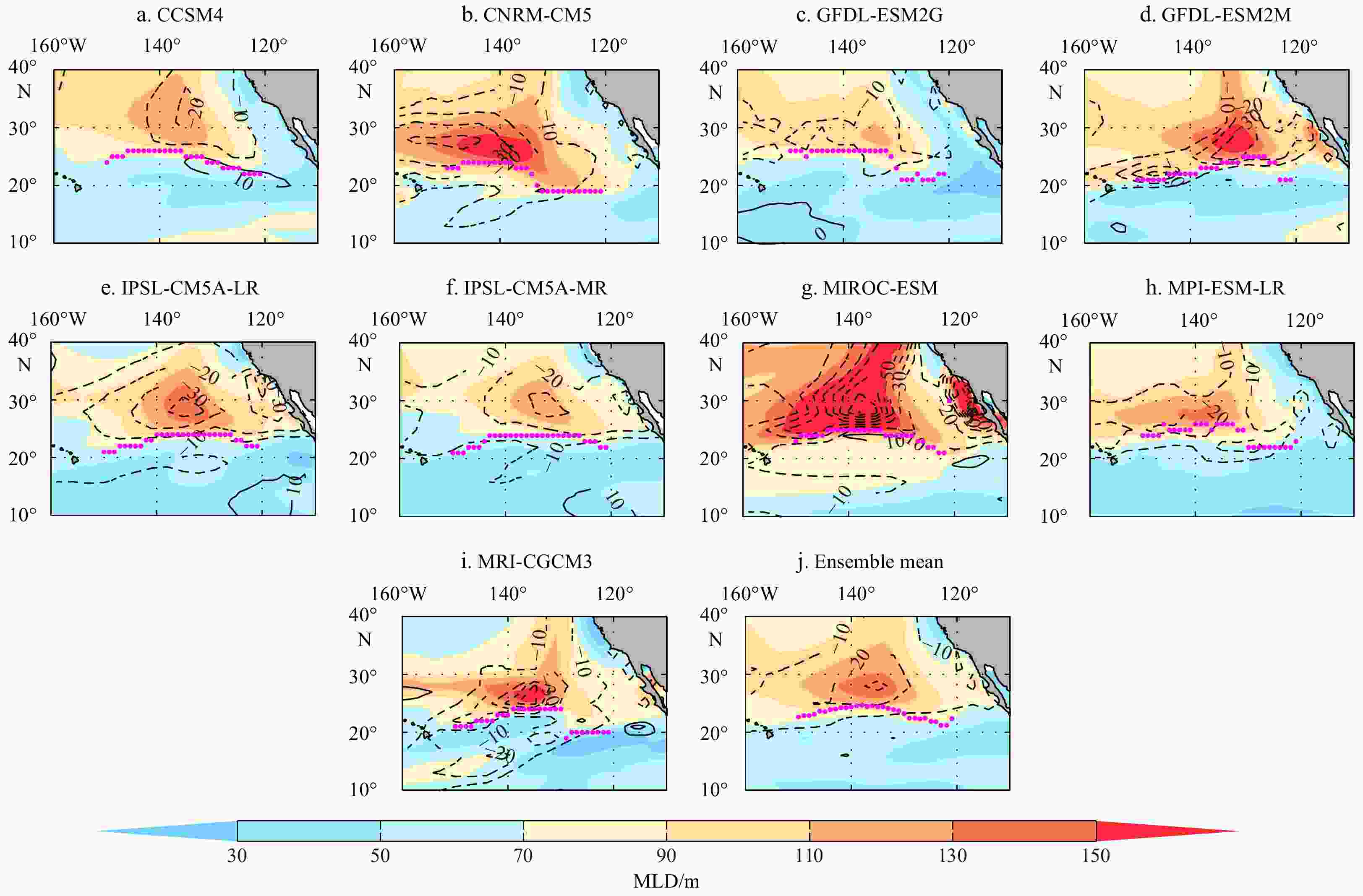
Figure 1. The February–March mean MLD (shading, interval: 20 m) from the historical simulation of the 9 models (a–i) and ensemble mean result (j). The contours indicate the mean MLD difference (RCP8.5 minus historical), dashed lines (negative values) means the MLD shoals in a much warmer climate. Magenta points represent the location of the MLD front in historical simulation.

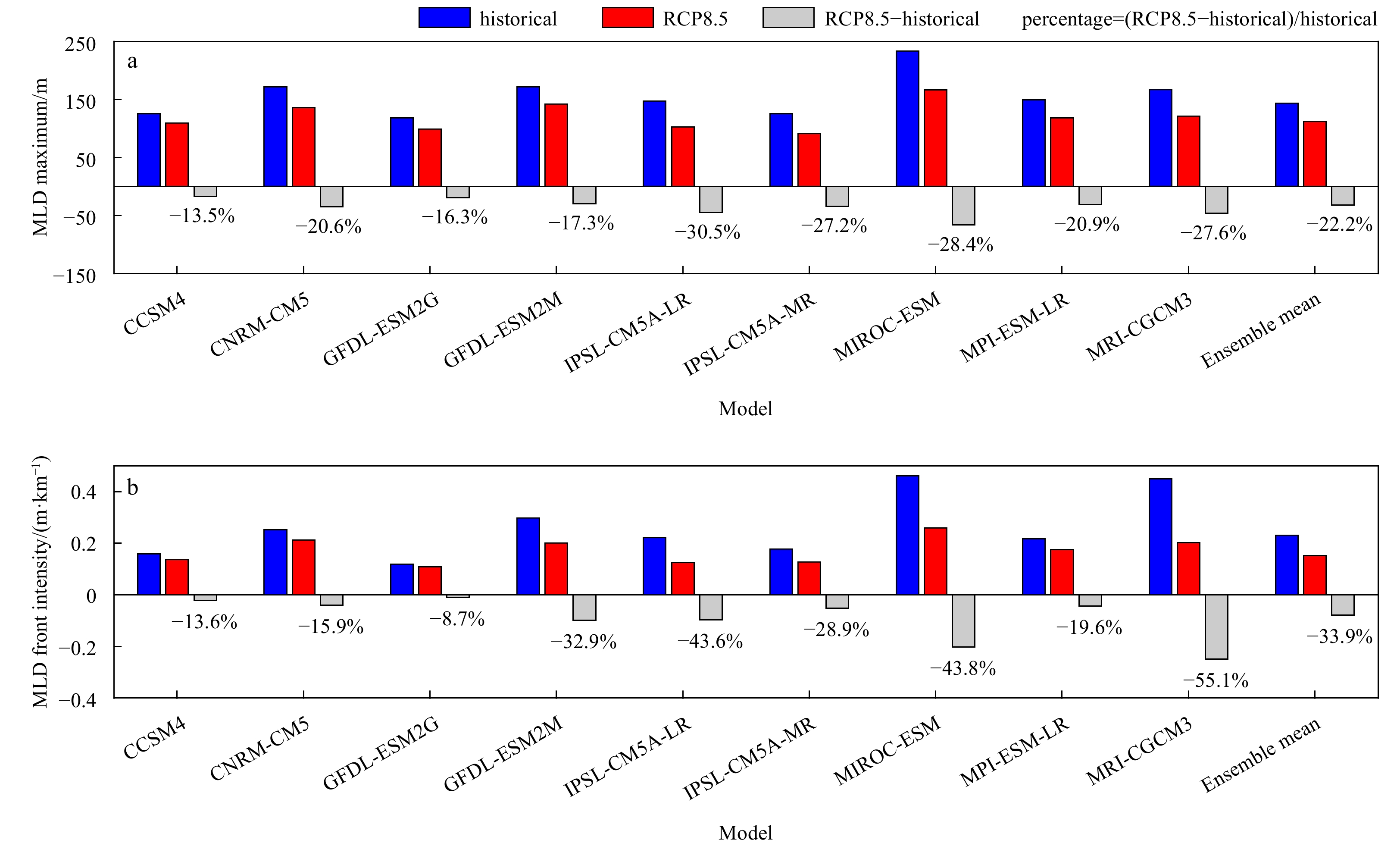
Figure 2. The MLD maximum (a), the intensity of the MLD front mean (b) during February–March in the 9 CMIP5 models and ensemble mean result. The colors represent historical simulation (blue), RCP8.5 experiment (red), and their differences (gray). Percentages represent changes compared to corresponding historical simulation.
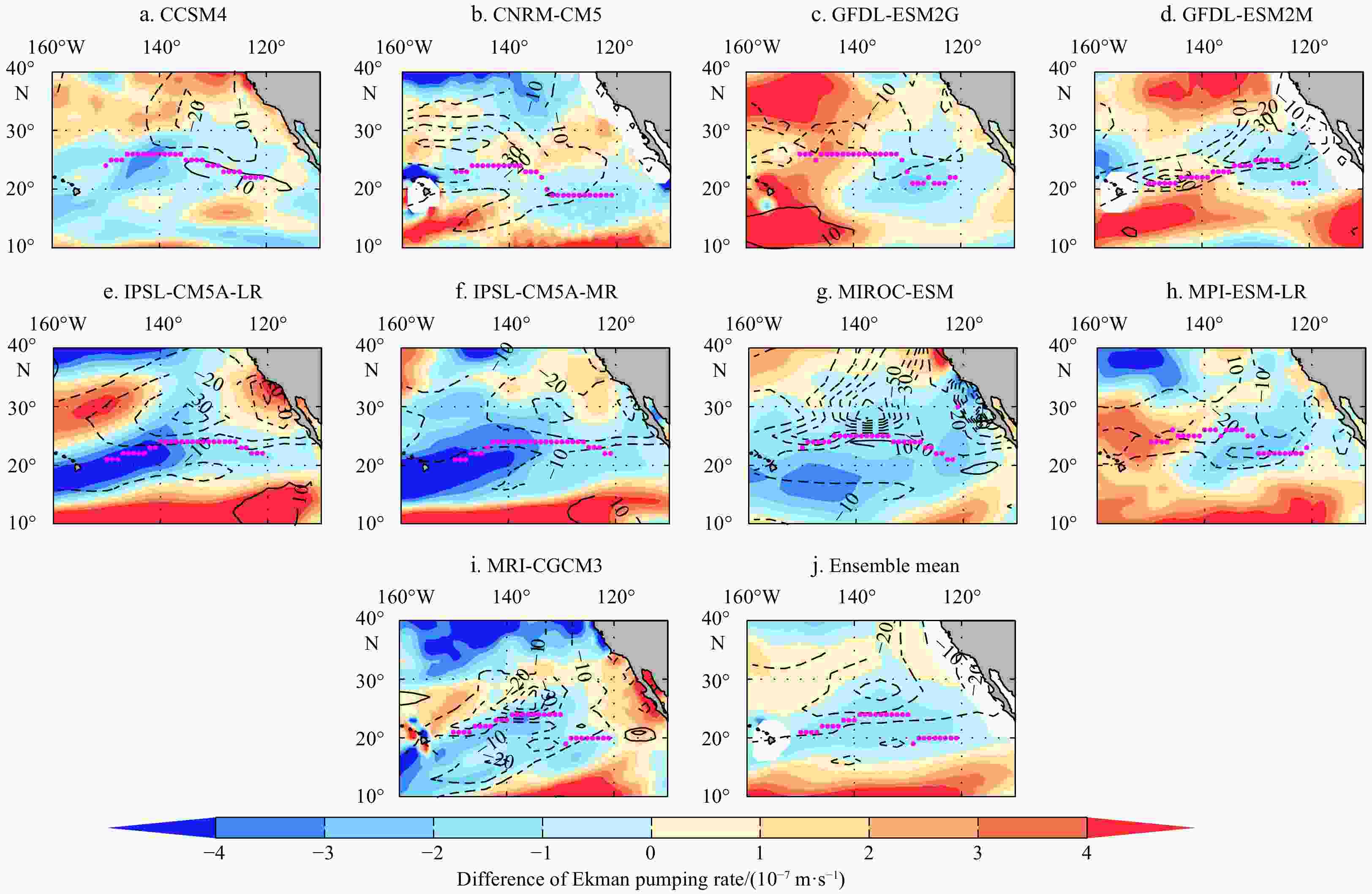
Figure 3. Differences (RCP 8.5 minus historical) of Ekman pumping rate (shading, downward is positive) mean during February–March of the 9 models (a–i) and ensemble mean result (j). The positive values indicate the Ekman pumping trend to downward and contribute to deepening the MLD. The contours indicate the difference (RCP8.5 minus historical) in MLD mean during February–March (contours, interval: 10 m). The magenta points represent the location of the MLD front in historical simulation.
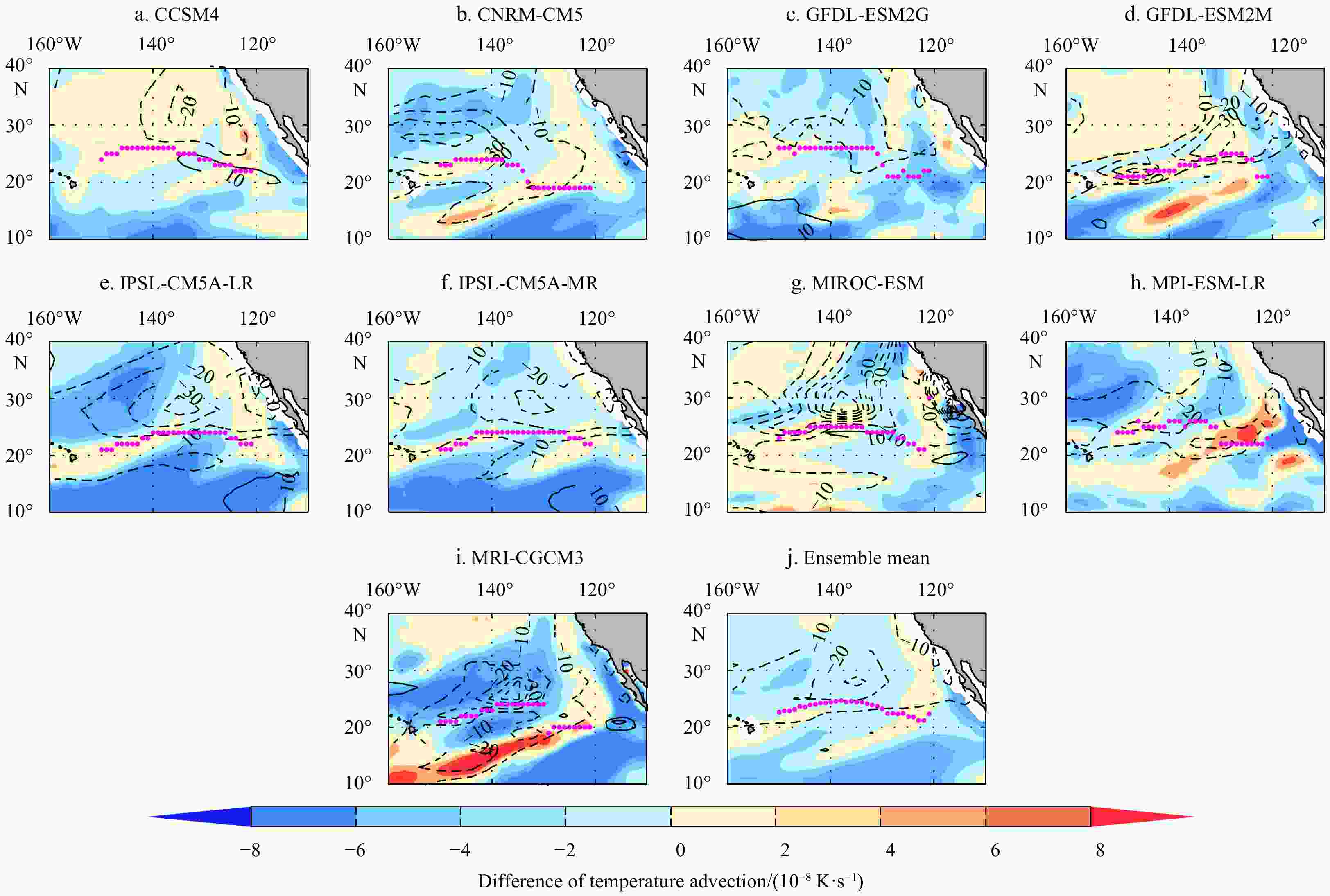
Figure 5. Differences (RCP 8.5 minus historical) of temperature advection (shading) mean during February–March of the 9 models (a–i) and ensemble mean result (j). The positive values indicate warm advection increased or cold advection decreased in the upper ocean and contribute to shoaling the MLD. The contours indicate the difference (RCP8.5 minus historical) in MLD mean during February–March (contours, interval: 10 m). The magenta points represent the location of the MLD front in historical simulation.
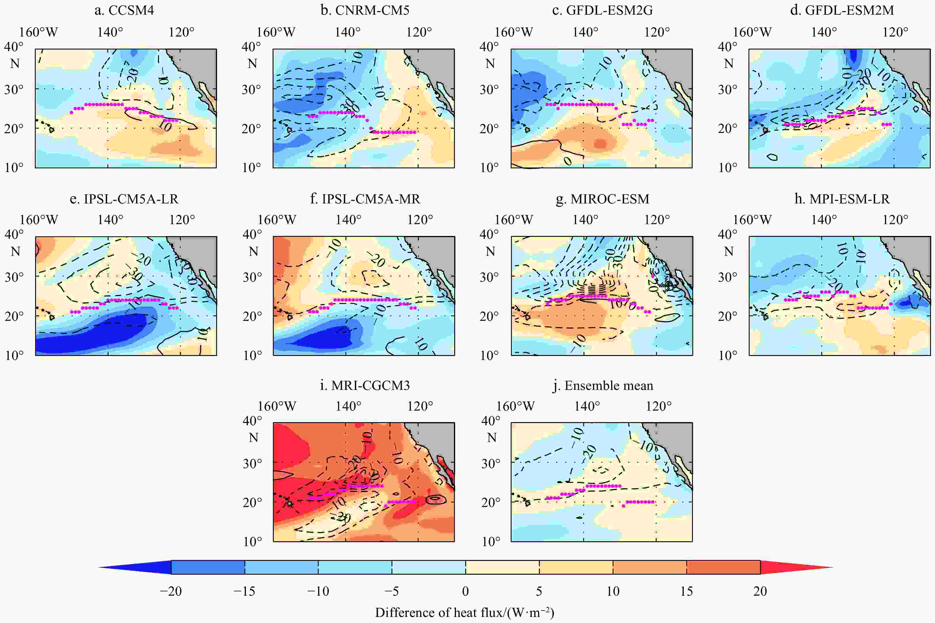
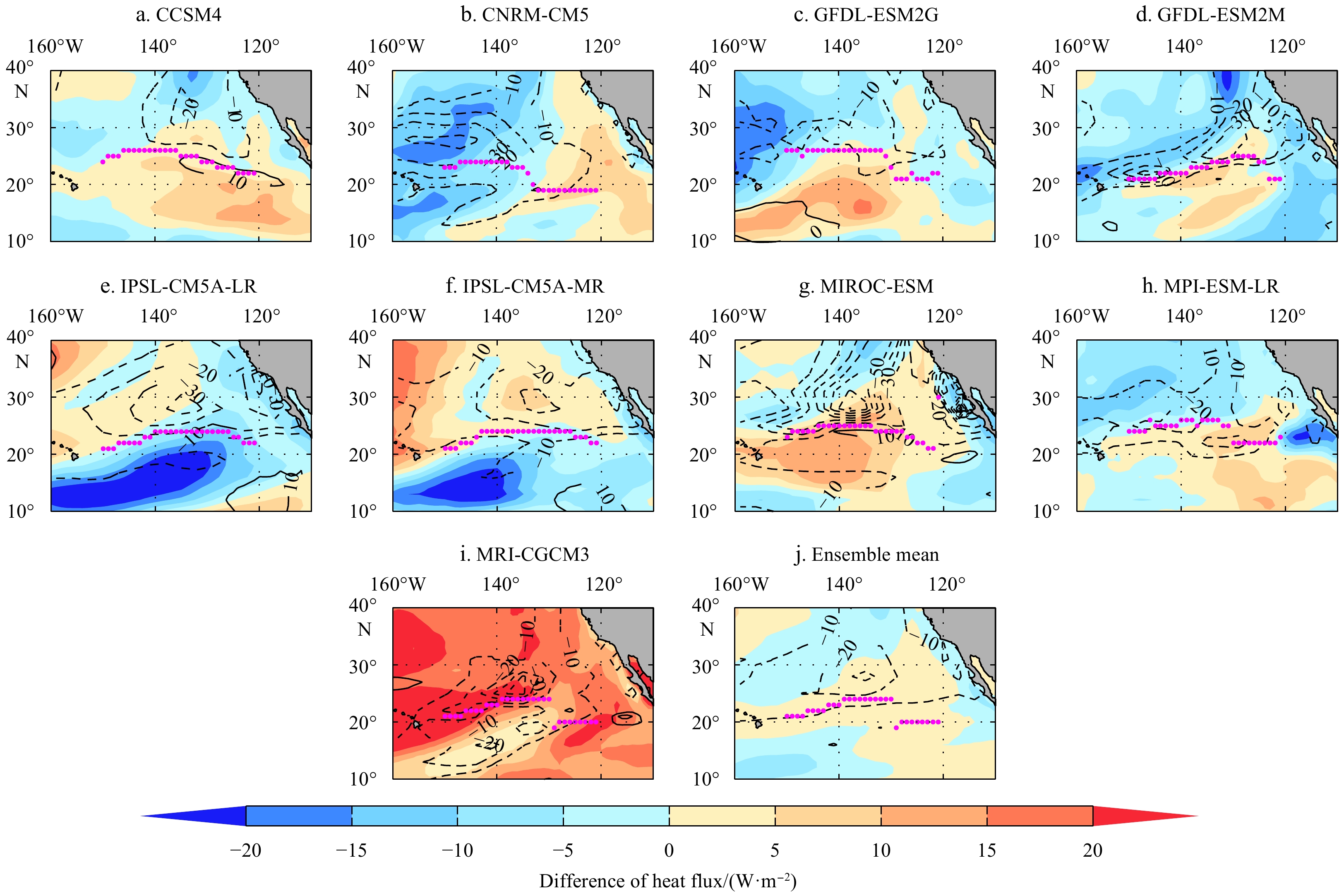
Figure 4. Differences (RCP 8.5 minus historical) of heat flux (shading) mean during February–March of the 9 models (a–i) and ensemble mean result (j). The positive values indicate the ocean release more heat to the atmosphere and contribute to deepening the MLD. The contours indicate the difference (RCP8.5 minus historical) in MLD mean during February–March (contours, interval: 10 m). The magenta points represent the location of the MLD front in historical simulation.
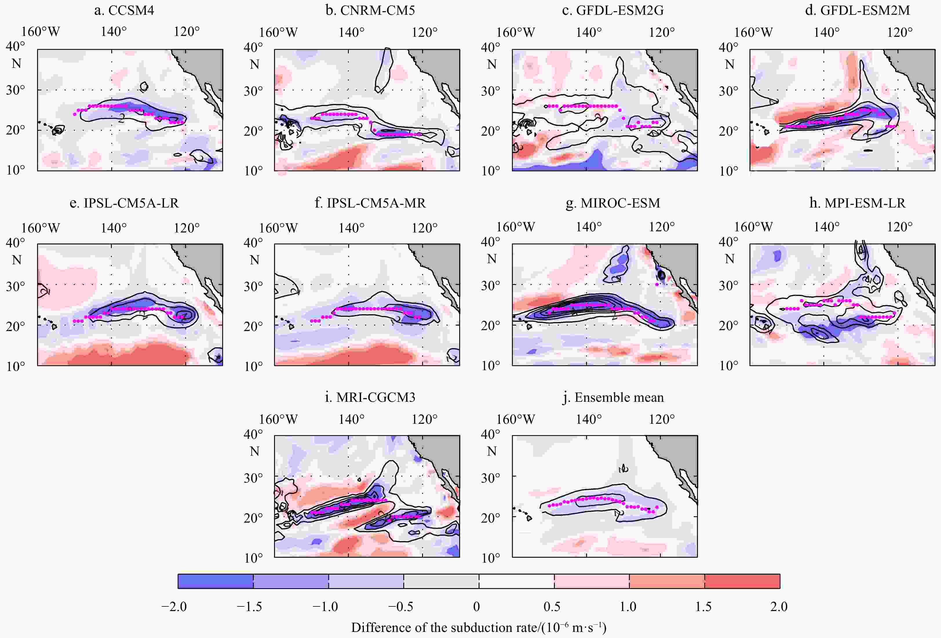
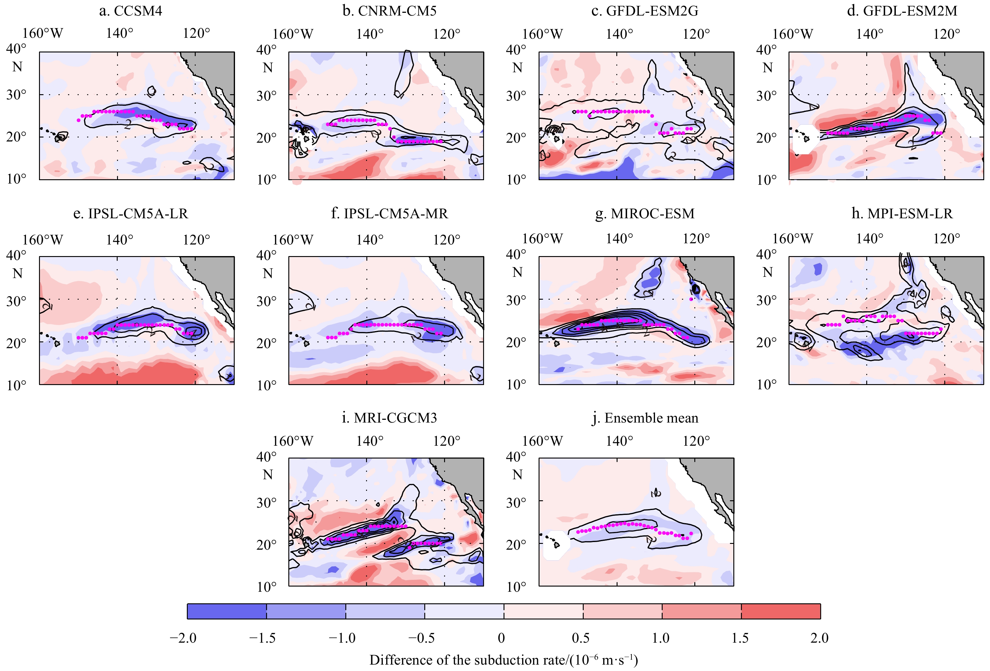
Figure 6. Differences (RCP 8.5 minus historical) of the subduction rate (shading, downward is positive) and subduction in historical simulation (contours, only over
$ 2\!\times\! {10}^{6} $ m/s are shown) during February–March in the 9 models (a–i) and ensemble mean (j) result. The magenta points represent the location of the MLD front in historical simulation.Table 1. The 9 models from CMIP5 analyzed in this study
Model Institution Country CCSM4 National Center for Atmospheric Research USA CNRM-CM5 Centre National de Recherches Meteorologiques France GFDL-ESM2G NOAA/Geophysical Fluid Dynamics Laboratory USA GFDL-ESM2M NOAA/Geophysical Fluid Dynamics Laboratory USA IPSL-CM5A-LR Institute Pierre-Simon Laplace France IPSL-CM5A-MR Institute Pierre-Simon Laplace France MIROC-ESM University of Tokyo Japan MPI-ESM-LR Max Planck Institute for Meteorology Germany MRI-CGCM3 Meteorological Research Institute Japan  下载: 导出CSV
Table 2. Qualitative comparison of the contribution of the three major factors to MLD change after global warming
ID Model Northern region Southern region Contribution of factor MLD
trendContribution of factor MLD
trend$ {w}_{\rm{e}} $ Q Tad $ {w}_{\rm{e}} $ Q Tad a CCSM4 + – – $ \downarrow $ + + + $ \uparrow $ b CNRM-CM5 + – + $ \downarrow $ + – – $ \downarrow $ c GFDL-ESM2G + – + $ \downarrow $ + + + $ \uparrow $ d GFDL-ESM2M + – – $ \downarrow $ + + – $ \downarrow $ e IPSL-CM5A-LR – + + $ \downarrow $ – – + $ \uparrow $ f IPSL-CM5A-MR – + + $ \downarrow $ – – + $ \uparrow $ g MIROC-ESM – + – $ \downarrow $ – + – $ \downarrow $ h MPI-ESM-LR + + – $ \downarrow $ + + – $ \downarrow $ i MRI-CGCM3 – + + $ \downarrow $ – + – $ \downarrow $ Note: $ {w}_{\rm{e}} $, Q, and Tad represent the Ekman pumping, net heat flux, and upper-ocean heat advection, respectively; + means it contributes to the MLD deepening, while – means it helps to shallow the MLD; the red color represents that factor is dominant to the actual MLD change; MLD trend represents the final change of MLD, $ \uparrow $ means the MLD deepened, and $ \downarrow $ means the MLD shallowed.
下载: 导出CSV
-
[1] Carton J A, Giese B S. 2008. A reanalysis of ocean climate using Simple Ocean Data Assimilation (SODA). Monthly Weather Review, 136(8): 2999–3017. doi: 10.1175/2007MWR1978.1 [2] Dawe J T, Thompson L A. 2007. PDO-related heat and temperature budget changes in a model of the North Pacific. Journal of Climate, 20(10): 2092–2108. doi: 10.1175/JCLI4229.1 [3] de Boyer Montégut C, Madec G, Fischer A S, et al. 2004. Mixed layer depth over the global ocean: An examination of profile data and a profile-based climatology. Journal of Geophysical Research: Oceans, 109(C12): C12003. doi: 10.1029/2004JC002378 [4] Dunne J P, John J G, Adcroft A J, et al. 2012. GFDL’s ESM2 global coupled climate-carbon earth system models: Part I, Physical formulation and baseline simulation characteristics. Journal of Climate, 25(19): 6646–6665. doi: 10.1175/JCLI-D-11-00560.1 [5] Hu Haibo, Liu Qinyu, Zhang Yuan, et al. 2011. Variability of subduction rates of the subtropical North Pacific mode waters. Chinese Journal of Oceanology and Limnology, 29(5): 1131–1141. doi: 10.1007/s00343-011-0237-x [6] Jang C J, Park J, Park T, et al. 2011. Response of the ocean mixed layer depth to global warming and its impact on primary production: a case for the North Pacific Ocean. ICES Journal of Marine Science, 68(6): 996–1007. doi: 10.1093/icesjms/fsr064 [7] Jiang Shunyu, Hu Haibo, Zhang Ning, et al. 2019. Multi-source forcing effects analysis using Liang–Kleeman information flow method and the community atmosphere model (CAM4.0). Climate Dynamics, 53(9): 6035–6053 [8] Kara A B, Rochford P A, Hurlburt H E. 2003. Mixed layer depth variability over the global ocean. Journal of Geophysical Research: Oceans, 108(C3): 3079. doi: 10.1029/2000JC000736 [9] Katsura S. 2018. Properties, formation, and dissipation of the North Pacific eastern Subtropical Mode Water and its impact on interannual spiciness anomalies. Progress in Oceanography, 162: 120–131. doi: 10.1016/j.pocean.2018.02.023 [10] Levitus S E. 1982. Climatological atlas of the World Ocean. NOAA Professional Paper 13. Washington DC: US Government Printing Office [11] Levitus S, Boyer T P. 1994. World Ocean Atlas 1994. Vol. 4. Temperature. Washington, DC: National Environmental Satellite, Data, and Information Service [12] Liu Qinyu, Lu Yiqun. 2016. Role of horizontal density advection in seasonal deepening of the mixed layer in the subtropical Southeast Pacific. Advances in Atmospheric Sciences, 33(4): 442–451. doi: 10.1007/s00376-015-5111-x [13] Liu Chengyan, Wang Zhaomin, Li Bingrui, et al. 2017. On the response of subduction in the South Pacific to an intensification of westerlies and heat flux in an eddy permitting ocean model. Advances in Atmospheric Sciences, 34(4): 521–531. doi: 10.1007/s00376-016-6021-2 [14] Marshall J C, Williams R G, Nurser A J G. 1993. Inferring the subduction rate and period over the North Atlantic. Journal of Physical Oceanography, 23(7): 1315–1329. doi: 10.1175/1520-0485(1993)023<1315:ITSRAP>2.0.CO;2 [15] Monterey G I, Levitus S. 1997. Climatological cycle of mixed layer depth in the world ocean. NOAA Atlas NESDIS 14. Washington, DC: US Government Printing Office [16] Pan Aijun, Wan Xiaofang, Liu Qinyu. 2011. Diagnostics of mixed-layer thermodynamics in the formation regime of the North Pacific subtropical mode water. Journal of Tropical Oceano- graphy (in Chinese), 30(5): 8–18 [17] Pond S, Pickard G L. 1983. Introductory Dynamical Oceanography. 2nd ed. New York: Pergamon, 379 [18] Qiu Bo, Chen Shuming. 2006. Decadal variability in the formation of the North Pacific Subtropical mode water: Oceanic versus atmospheric control. Journal of Physical Oceanography, 36(7): 1365–1380. doi: 10.1175/JPO2918.1 [19] Qiu Bo, Kelly K A. 1993. Upper-ocean heat balance in the Kuroshio extension region. Journal of Physical Oceanography, 23(9): 2027–2041. doi: 10.1175/1520-0485(1993)023<2027:UOHBIT>2.0.CO;2 [20] Qu Tangdong, Chen Ju. 2009. A North Pacific decadal variability in subduction rate. Geophysical Research Letters, 36(22): L22602. doi: 10.1029/2009GL040914 [21] Somavilla R, González-Pola C, Fernández-Diaz J. 2017. The warmer the ocean surface, the shallower the mixed layer. How much of this is true?. Journal of Geophysical Research: Oceans, 122(9): 7698–7716. doi: 10.1002/2017JC013125 [22] Stommel H. 1979. Determination of water mass properties of water pumped down from the Ekman layer to the geostrophic flow below. Proceedings of the National Academy of Sciences of the United States of America, 76(7): 3051–3055. doi: 10.1073/pnas.76.7.3051 [23] Taylor K E, Stouffer R J, Meehl G A. 2012. An overview of CMIP5 and the experiment design. Bulletin of the American Meteorological Society, 93(4): 485–498. doi: 10.1175/BAMS-D-11-00094.1 [24] van Vuuren D P, Edmonds J, Kainuma M, et al. 2011. The representative concentration pathways: An overview. Climatic Change, 109(1): 5 [25] Wang Ran, Cheng Xuhua, Xu Lixiao, et al. 2020a. Mesoscale eddy effects on the subduction of North Pacific eastern subtropical mode water. Journal of Geophysical Research: Oceans, 125(5): e2019JC015641 [26] Wang Ziyi, Wen Zhibin, Hu Haibo, et al. 2020b. The characteristics of near‐equatorial North Pacific Low PV water and its possible influences on the Equatorial Subsurface Ocean. Journal of Geophysical Research: Oceans, 125(9): e2020JC016282 [27] Wen Zhibin, Hu Haibo, Song Zhenya, et al. 2020. Different influences of mesoscale oceanic eddies on the North Pacific subsurface low potential vorticity water mass between winter and summer. Journal of Geophysical Research: Oceans, 125(1): e2019JC015333 [28] Williams R G. 1991. The role of the mixed layer in setting the potential vorticity of the main thermocline. Journal of Physical Oceanography, 21(12): 1803–1814. doi: 10.1175/1520-0485(1991)021<1803:TROTML>2.0.CO;2 [29] Woods J D. 1985. The physics of pycnocline ventilation. In: Nihoul J C J, ed. Coupled Ocean-Atmosphere Models. London: Elsevier, 543–590 [30] Xia Ruibin, Liu Chengyan, Cheng Chen. 2018. On the subtropical Northeast Pacific mixed layer depth and its influence on the subduction. Acta Oceanologica Sinica, 37(3): 51–62. doi: 10.1007/s13131-017-1102-3 [31] Xia Ruibin, Liu Qinyu, Xu Lixiao, et al. 2015. North Pacific Eastern Subtropical Mode Water simulation and future projection. Acta Oceanologica Sinica, 34(3): 25–30. doi: 10.1007/s13131-015-0630-y [32] Xie S-P, Deser C, Vecchi G A, et al. 2010. Global warming pattern formation: sea surface temperature and rainfall. Journal of Climate, 23(4): 966–986. doi: 10.1175/2009JCLI3329.1 [33] Xu Lixiao, Li Peiliang, Xie S-P, et al. 2016. Observing mesoscale eddy effects on mode-water subduction and transport in the North Pacific. Nature Communications, 7(1): 10505. doi: 10.1038/ncomms10505 [34] Xu Lixiao, Xie S-P, Liu Qinyu. 2012. Mode water ventilation and subtropical countercurrent over the North Pacific in CMIP5 simulations and future projections. Journal of Geophysical Research: Oceans, 117(C12): C12009 [35] Xu Lixiao, Xie S-P, Liu Qinyu, et al. 2017. Evolution of the North Pacific subtropical mode water in anticyclonic eddies. Journal of Geophysical Research: Oceans, 122(C12): 10118–10130 [36] Zhang Ruosi, Xie S-P, Xu Lixiao, et al. 2016. Changes in mixed layer depth and spring bloom in the Kuroshio Extension under global warming. Advances in Atmospheric Sciences, 33(4): 452–461. doi: 10.1007/s00376-015-5113-8 -


 点击查看大图

计量
- 文章访问数: 688
- HTML全文浏览量: 235
- PDF下载量: 20
- 被引次数: 0