

Simulation and future projection of the mixed layer depth and subduction process in the subtropical Southeast Pacific
-
Abstract: The present climate simulation and future projection of the mixed layer depth (MLD) and subduction process in the subtropical Southeast Pacific are investigated based on the geophysical fluid dynamics laboratory earth system model (GFDL-ESM2M). The MLD deepens from May and reaches its maximum (>160 m) near (24°S, 104°W) in September in the historical simulation. The MLD spatial pattern in September is non-uniform in the present climate, which shows three characteristics: (1) the deep MLD extends from the Southeast Pacific to the West Pacific and leads to a “deep tongue” until 135°W; (2) the northern boundary of the MLD maximum is smoothly near 18°S, and MLD shallows sharply to the northeast; (3) there is a relatively shallow MLD zone inserted into the MLD maximum eastern boundary near (26°S, 80°W) as a weak “shallow tongue”. The MLD non-uniform spatial pattern generates three strong MLD fronts respectively in the three key regions, promoting the subduction rate. After global warming, the variability of MLD spatial patterns is remarkably diverse, rather than deepening consistently. In all the key regions, the MLD deepens in the south but shoals in the north, strengthing the MLD front. As a result, the subduction rate enhances in these areas. This MLD antisymmetric variability is mainly influenced by various factors, especially the potential-density horizontal advection non-uniform changes. Notice that the freshwater flux change helps to deepen the MLD uniformly in the whole basin, so it hardly works on the regional MLD variability. The study highlights that there are regional differences in the mechanisms of the MLD change, and the MLD front change caused by MLD non-uniform variability is the crucial factor in the subduction response to global warming.
-
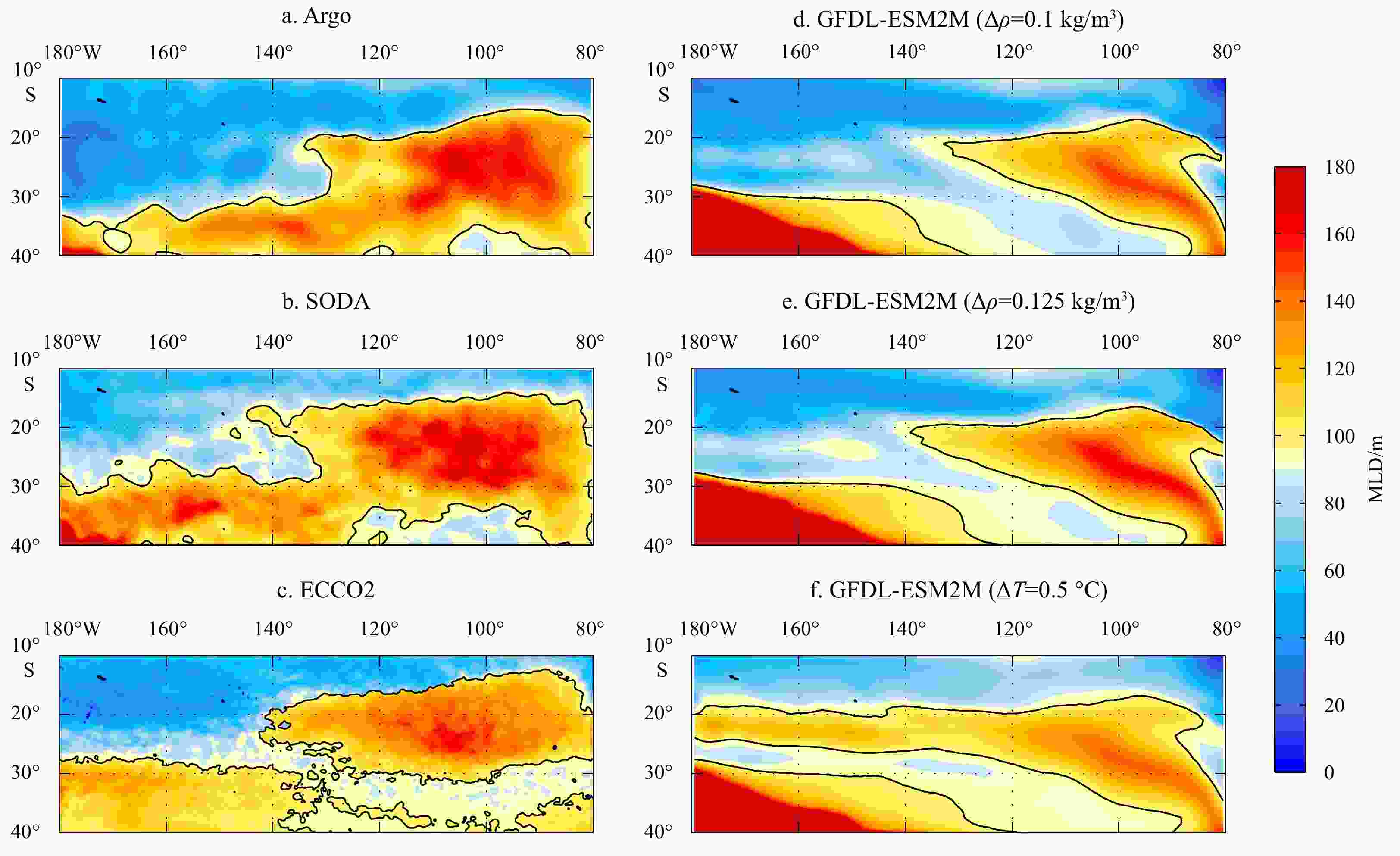
Figure 1. The September mean mixed layer depth (MLD, shading) based on Argo (a), SODA (b), ECCO2 (c), and GFDL-ESM2M (d–f, with different MLD definition). The MLD in a–d is defined by
$ \Delta \rho =0.1 $ kg/m3, and the MLD in e and f are defined by$\Delta \rho=0.125 $ kg/m3 and$\Delta T=0.5 $ °C, respectively. The bold black contours (100 m MLD) represent the MLD front roughly.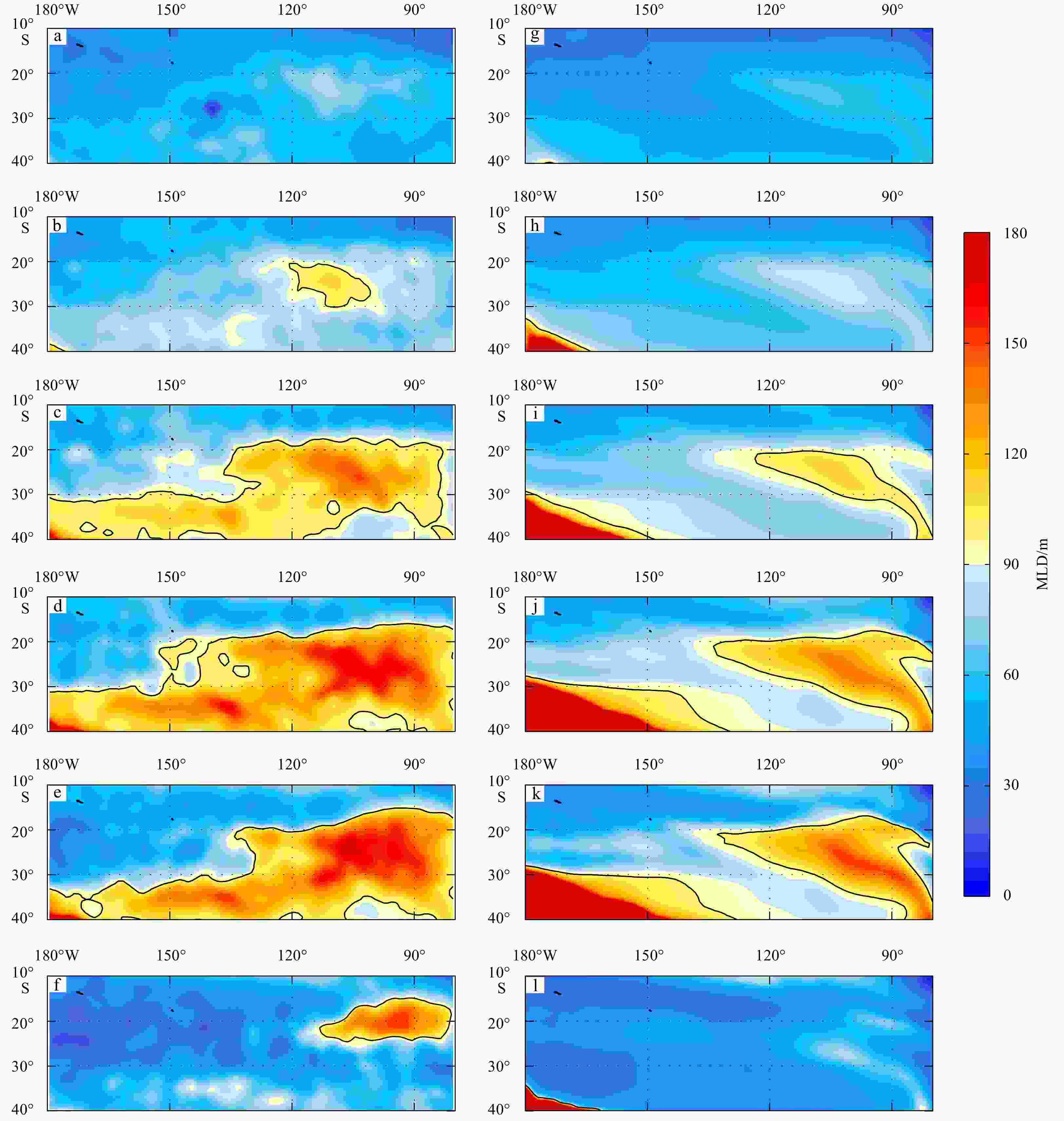
Figure 2. Monthly mean mixed layer depth (MLD, shading) in May (a, g), June (b, h), July (c, i), August (d, j), September (e, k), and October (f, l) based on Argo (a–f), and GFDL-ESM2M (g–l). The bold black contours (100 m MLD) represent the MLD front roughly.

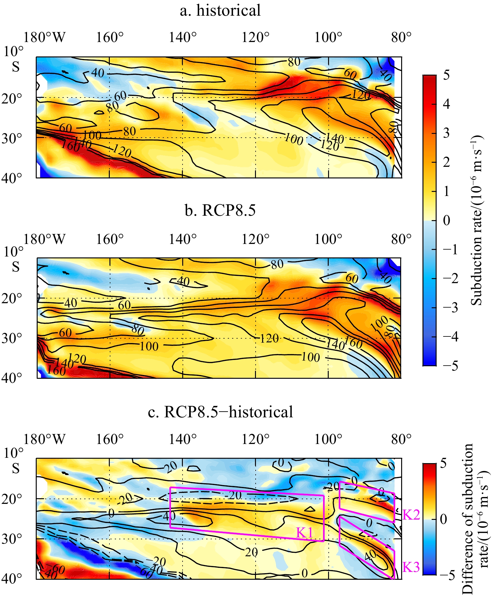
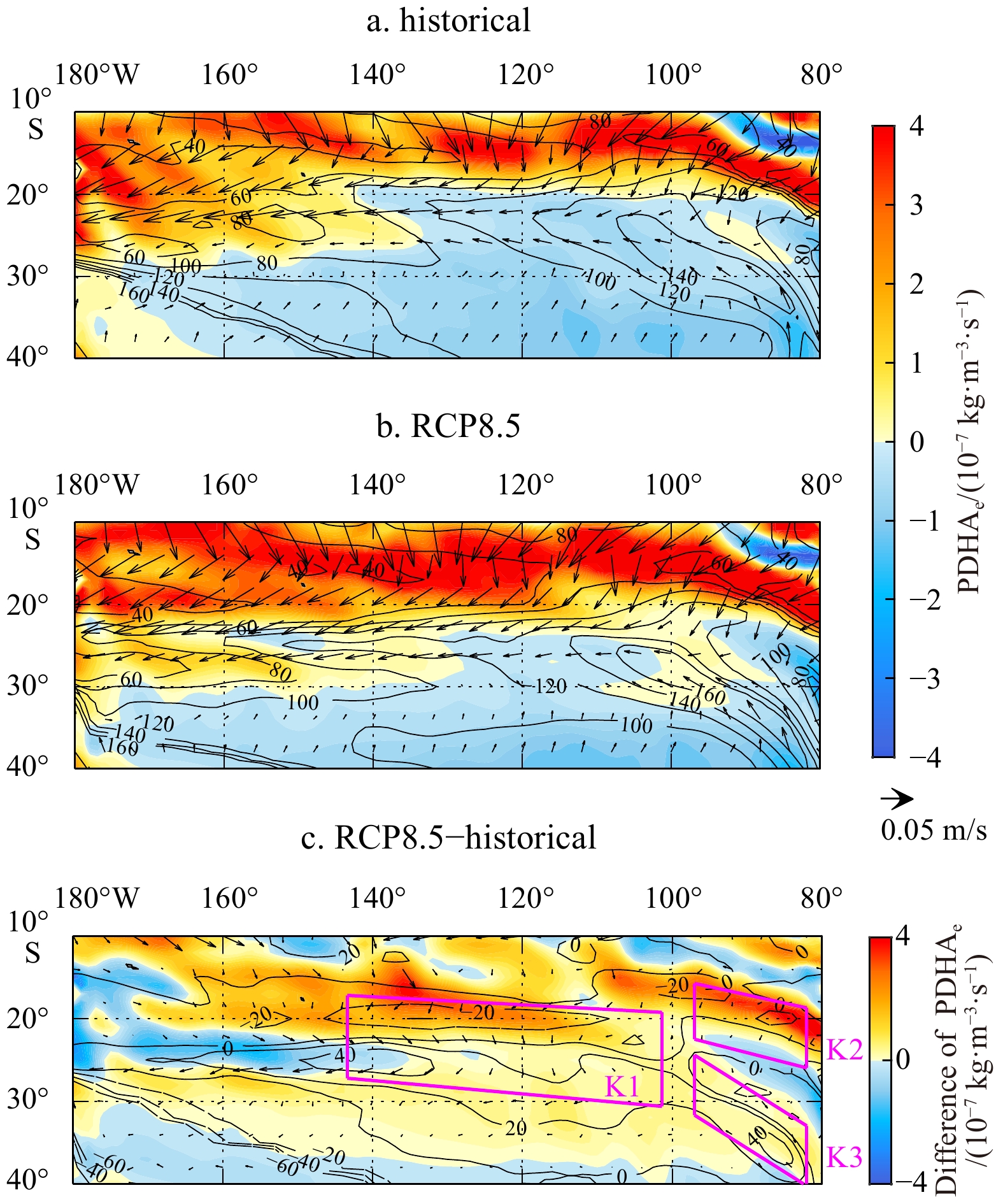
Figure 3. The mean mixed layer depth (MLD, contours, interval 20 m) and subduction rate (shading, positive means subduction) in September in historical simulation (a) and RCP8.5 experiment (b); and the differences of MLD (contours, interval: 20 m) and subduction rate (shading) between two scenarios (RCP 8.5 minus historical) (c). Magenta frames in c represent the three key regions where subduction increases significantly in the SEP, marked as K1, K2 and K3, respectively. In c, positive subduction rate means subduction increases.
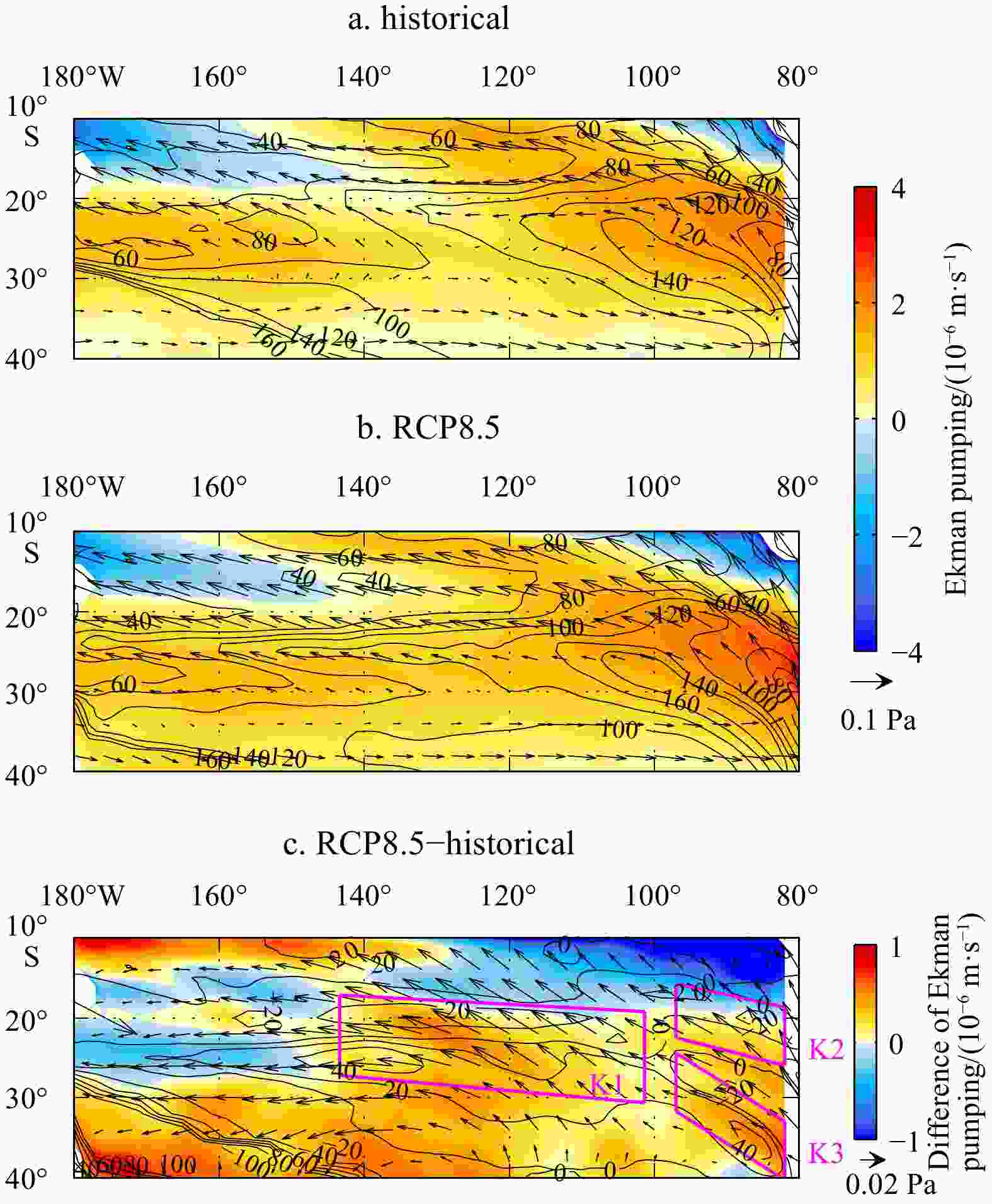
Figure 4. The mean mixed layer depth (MLD, contours, interval 20 m), wind stress (vectors), and Ekman pumping (shading, downward is positive, contribute to deepening the MLD) in September in historical simulation (a) and RCP8.5 experiment (b); and the differences of wind stress (vectors) and Ekman pumping (shading) between two scenarios (RCP 8.5 minus historical) (c). Magenta frames in c represent the three key regions defined in Fig. 3. In a and b, positive subduction rate means subduction, and in c, postive Ekman pumping means the downward Ekman pumping increases.
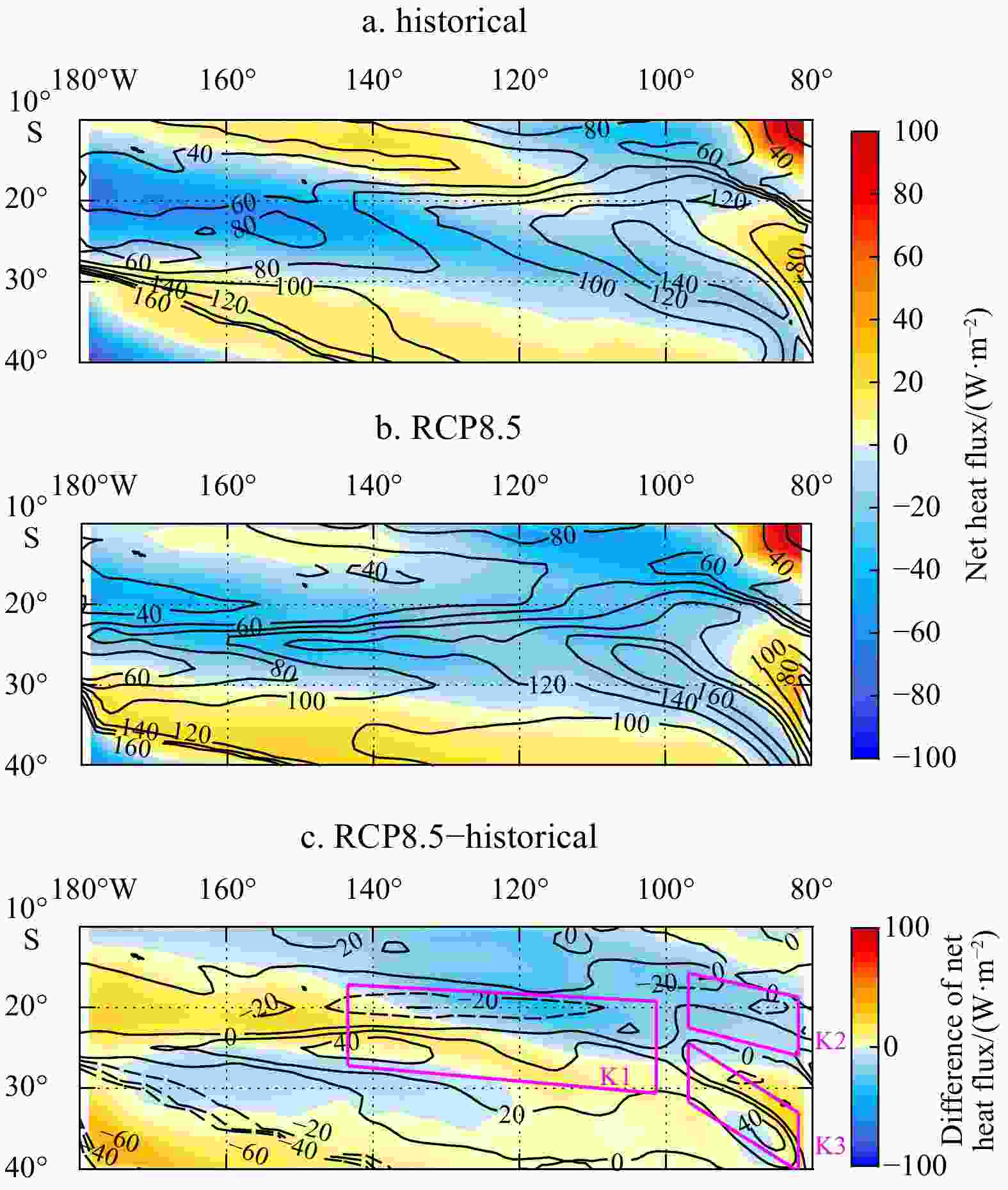
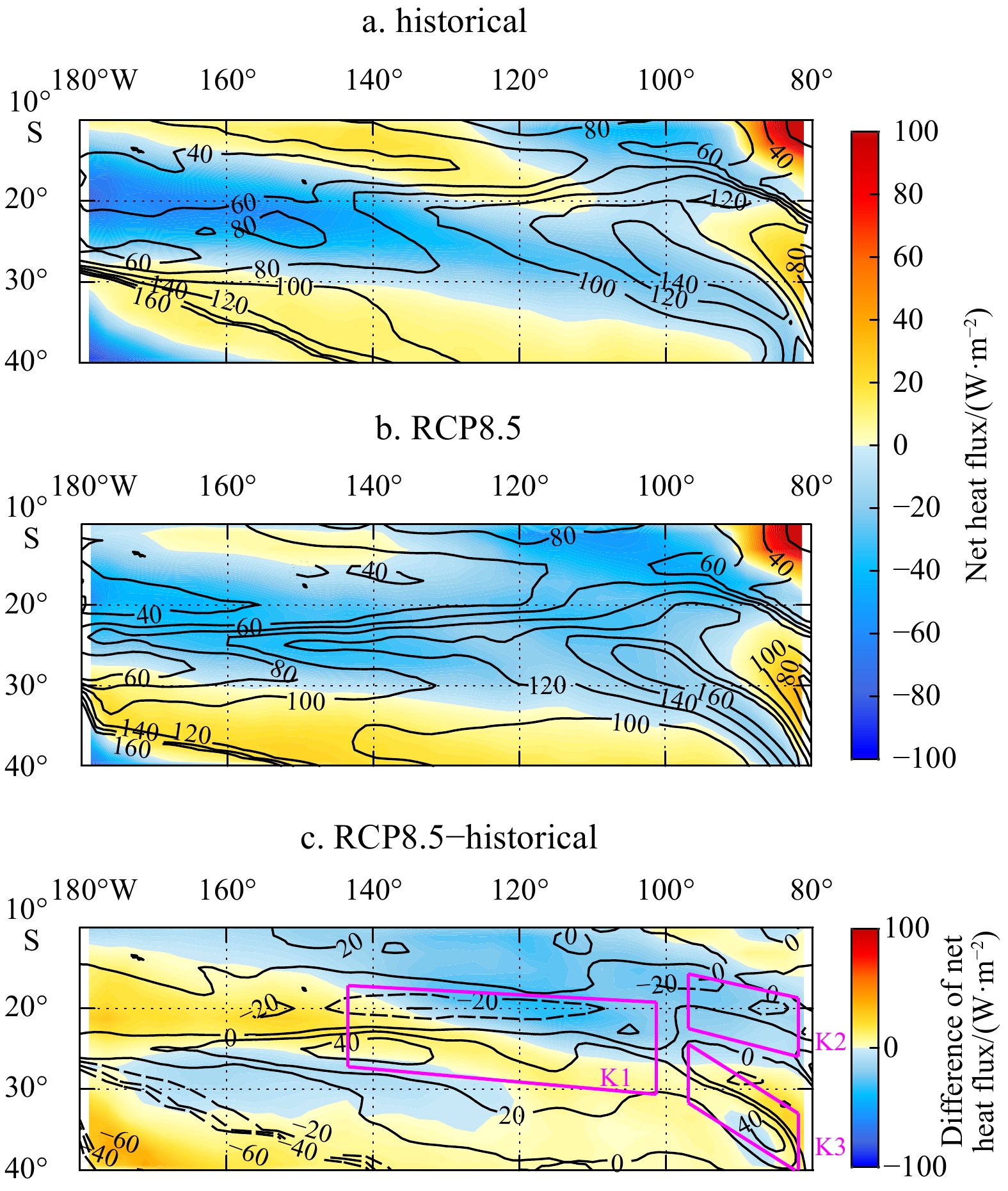
Figure 5. The mean mixed layer depth (MLD, contours, interval 20 m) and net heat flux from the atmosphere to ocean (shading) in September in historical simulation (a) and RCP8.5 experiment (b); and the differences of MLD and net heat flux (shading, unit: W/m2) between two scenarios (RCP 8.5 minus historical) (c). Magenta frames in c represent the three regions defined in Fig. 3. In a and b, positive net heat flux means ocean get heat and helps to shallow the MLD, and in c positive difference of netheat flux means ocean get more heat.
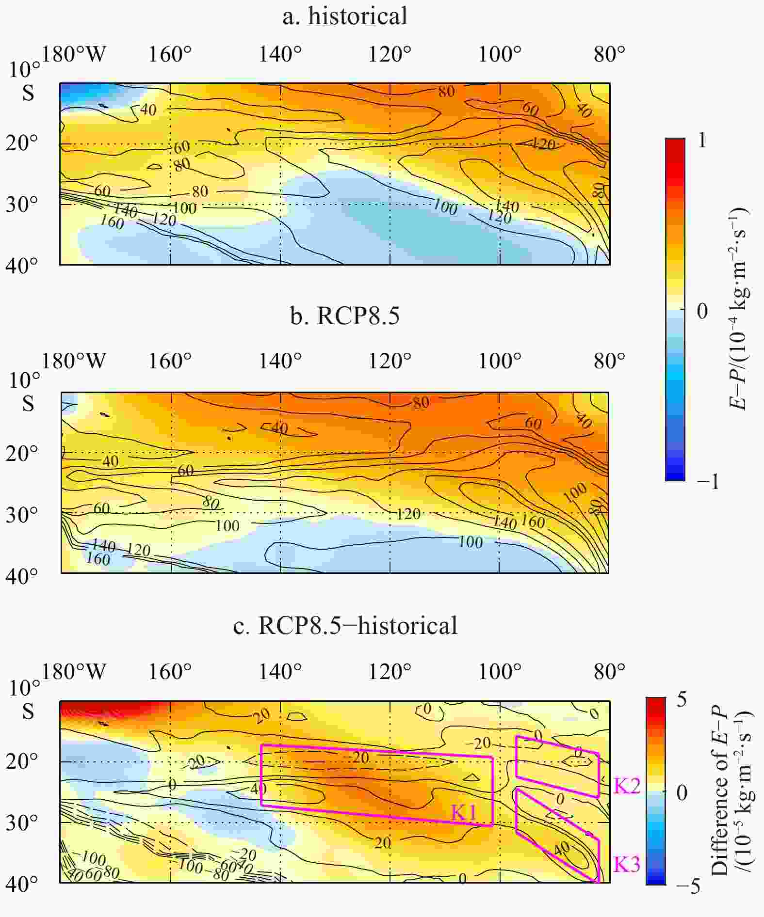
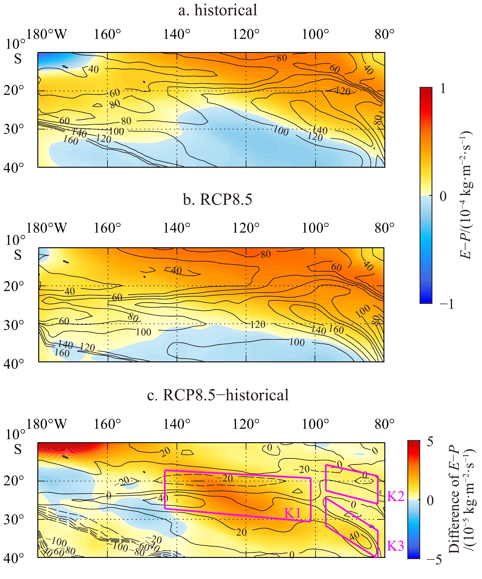
Figure 6. The mean mixed layer depth (MLD, contours, interval 20 m) and E−P flux (evaporation minus precipitation) from the atmosphere to ocean (shading) in September in historical simulation (a) and RCP8.5 experiment (b); and the differences of MLD and E−P flux (shading) between two scenarios (RCP 8.5 minus historical) (c). Magenta frames in c represent the three regions defined in Fig. 3. In a and b, positive E−P flux means the upper ocean salinity increasing and helps to deepen the MLD, and in c, positive difference of E−P flux means ocean becomes saltier.
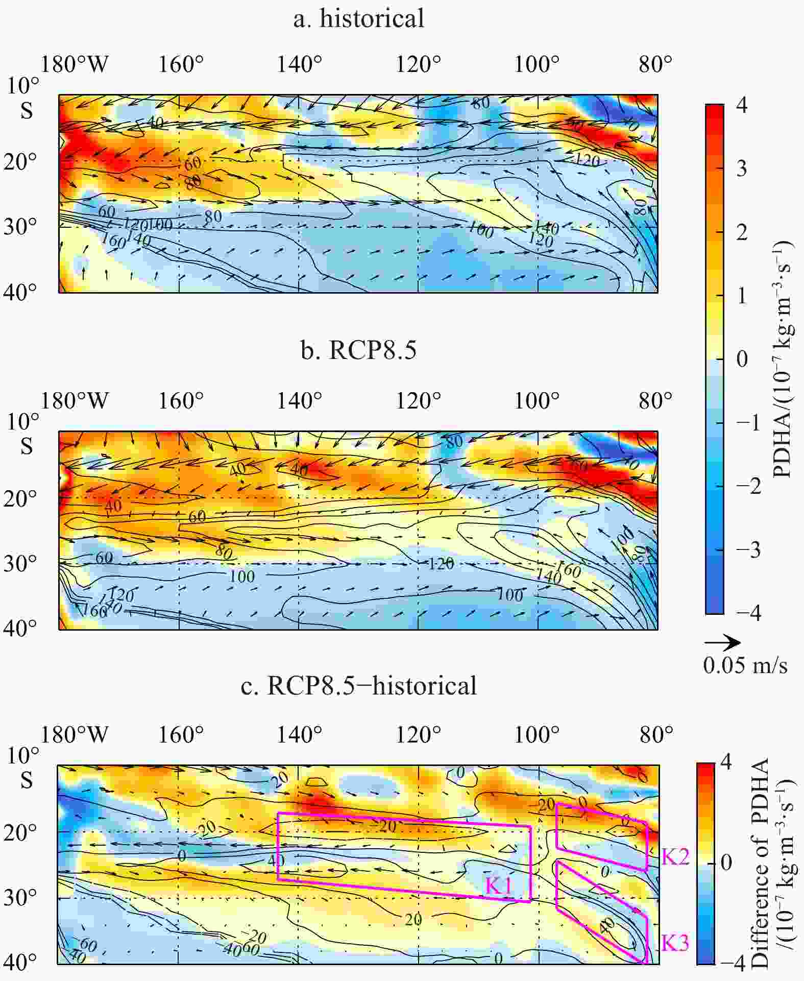
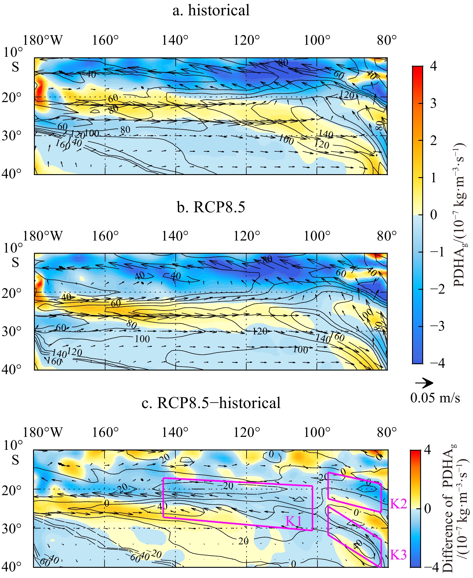
Figure 7. The mean mixed layer depth (MLD, contours, interval 20 m), the vertical average velocity (vectors), and the PDHA (shading, vertical integration above 100 m, positive values help MLD shoals) in September in historical simulation (a) and RCP8.5 experiment (b); and the differences of MLD, the vertical average velocity, and the PDHA (shading) between two scenarios (RCP 8.5 minus historical) (c). Magenta frames in c represent the three regions defined in Fig. 3.
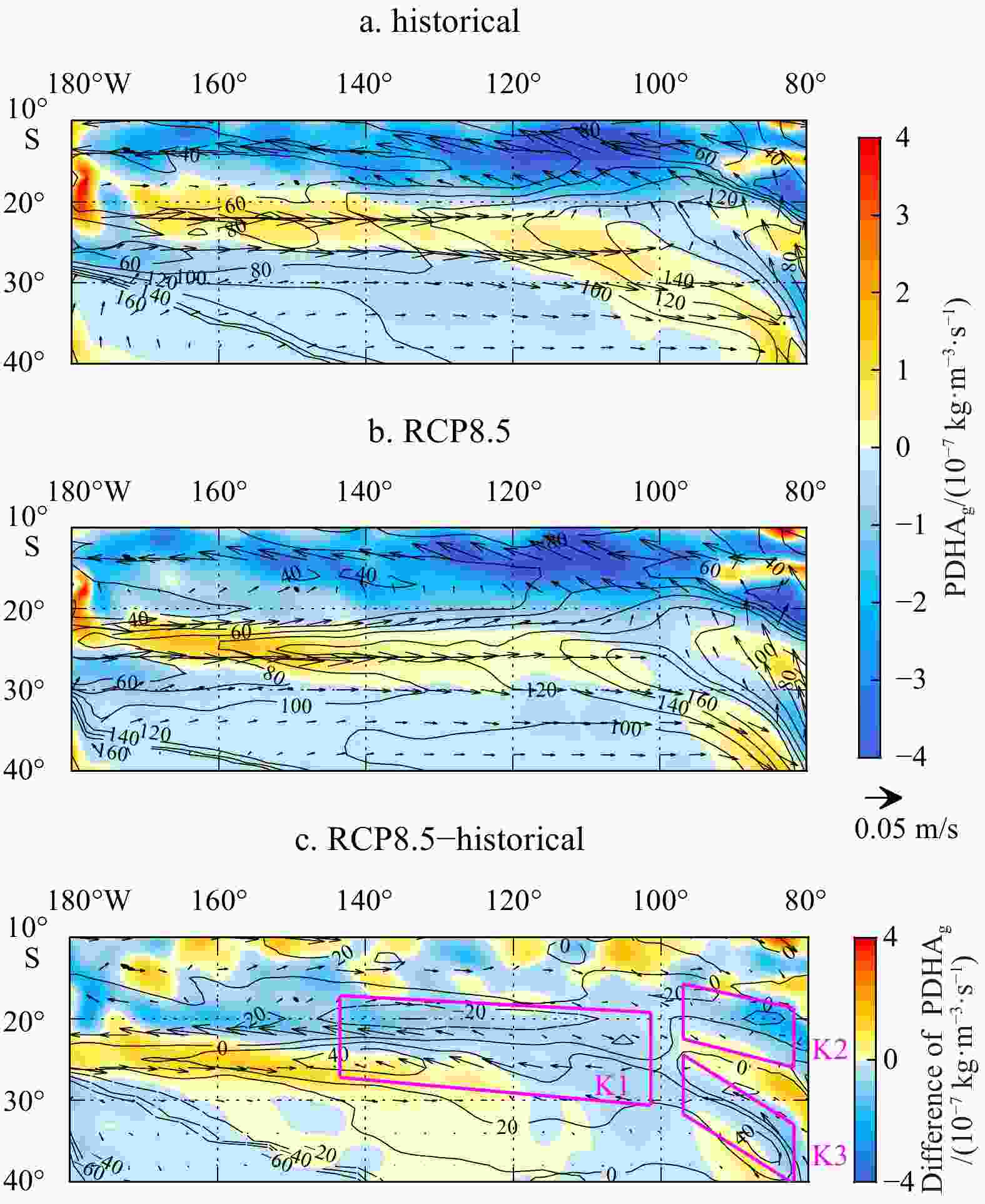
Figure 8. The mean mixed layer depth (MLD, contours, interval 20 m), the vertical average geostrophic velocity (vectors) and the
$ {\mathrm{P}\mathrm{D}\mathrm{H}\mathrm{A}}_{\mathrm{g}} $ (shading, vertical integration above 100 m, positive values help MLD shoals) in September in historical simulation (a) and RCP8.5 experiment (b); and the differences of MLD, the vertical average geostrophic velocity and the$ {\mathrm{P}\mathrm{D}\mathrm{H}\mathrm{A}}_{\mathrm{g}} $ (shading) between two scenarios (RCP 8.5 minus historical) (c). Magenta frames in c represent the three regions defined in Fig. 3.
Figure 9. The mean mixed layer depth (MLD, contours, interval 20 m), the vertical average Ekman horizontal velocity (vectors) and the
$ {\mathrm{P}\mathrm{D}\mathrm{H}\mathrm{A}}_{\mathrm{e}} $ (shading, vertical integration above 100 m, positive values help MLD shoals) in September in historical simulation (a) and RCP8.5 experiment (b); and the differences of MLD, the vertical average Ekman horizontal velocity and the$ {\mathrm{P}\mathrm{D}\mathrm{H}\mathrm{A}}_{\mathrm{e}} $ (shading) between two scenarios (RCP 8.5 minus historical) (c). Magenta frames in c represent the three regions defined in Fig. 3.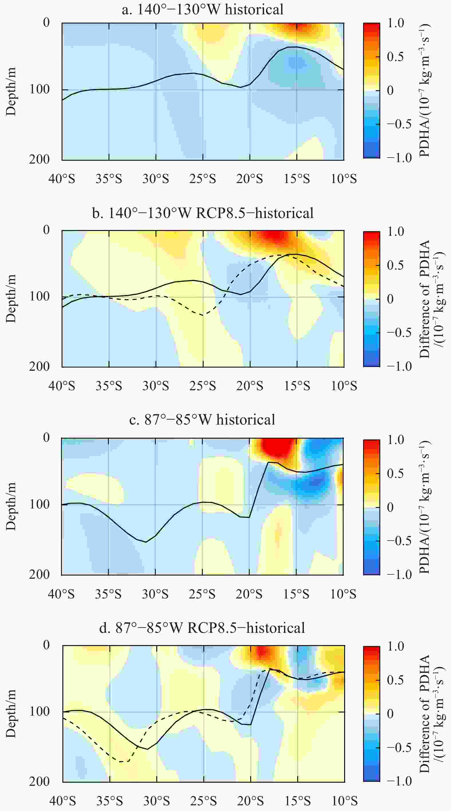
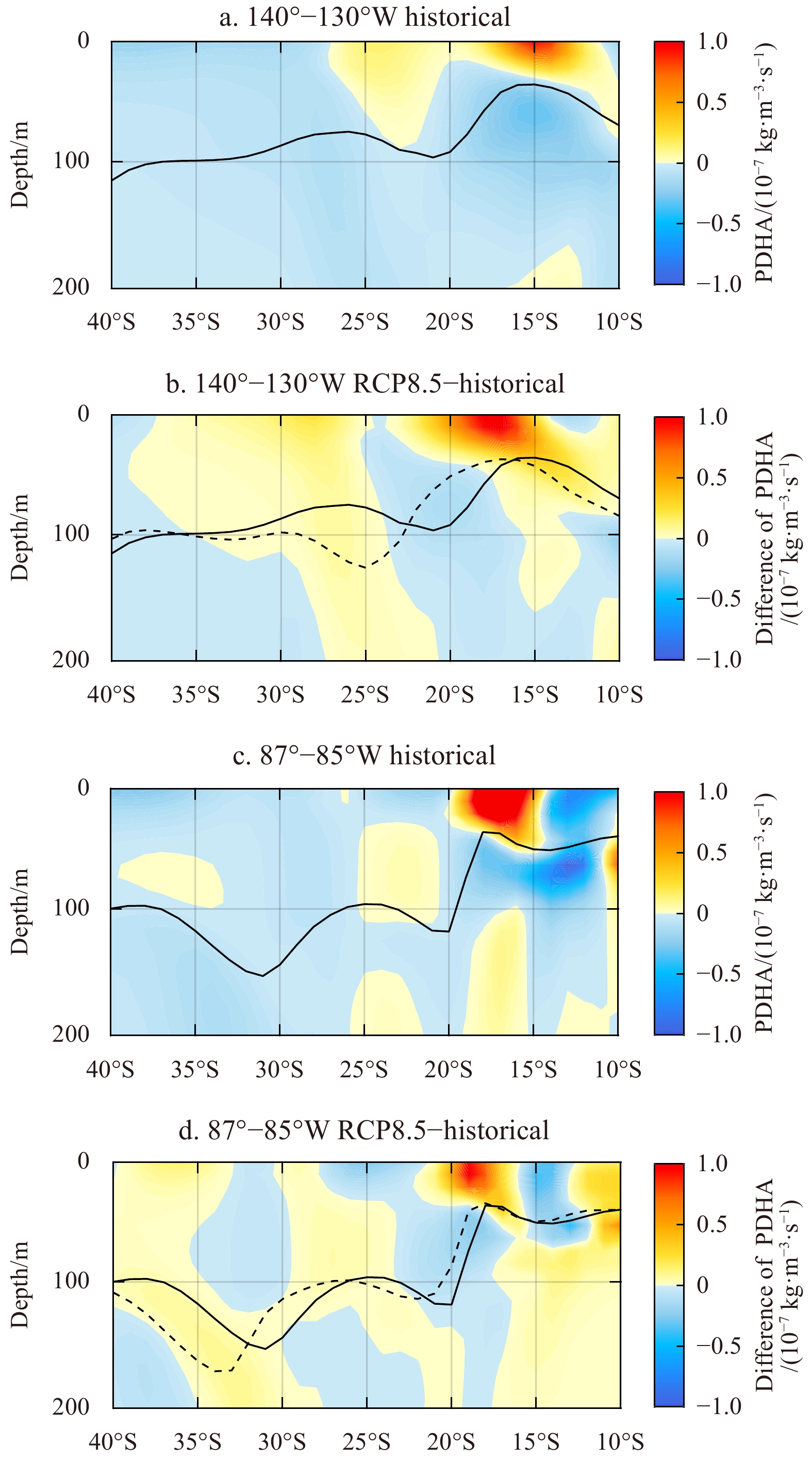
Figure 10. Depth-latitude section of PDHA (shading) along 140°W to 130°W (a, b) and along 87°W to 85°W (c, d). a and c. the present climate, and b and d. The change after global warming (RCP8.5 minus historical). Superimposed are the MLD in historical (black lines) and RCP8.5 (dashed lines). We check the PDHA in Region K1 from a and b, and Regions K2 and K3 from c and d.
Table 1. Qualitative comparison of the contributions of major factors to the MLD change after global warming
Variable Region K1 Region K2 Region K3 North South North South North South ΔMLD ↓ ↑ ↓ ↑ ↓ ↑ $ \Delta {w}_{\mathrm{e}} $ ↑ ↑ ↓ ↑ ↑ ↑ ΔQ ↓ ↑ ↓ ↓ ↑ ↓ Δ(E−P) ↑ ↑ ↑ ↑ ↑ ↑ ΔPDHA ↑ ↑ ↑ ↓ ↓ ↑ ΔPDHAg ↓ ↓ ↓ ↓ ↓ ↓ ΔPDHAe ↑ ↑ ↑ ↓ ↑ ↑ Note: Regions K1, K2 and K3 are the three key regions defined in Fig. 3c. ΔMLD, $ {\Delta w}_{\mathrm{e}} $, ΔQ, Δ(E−P), ΔPDHA represent the changes of mixed layer depth, Ekman pumping (positive values help the MLD deepening), net heat flux from the atmosphere to the ocean (positive values help the MLD shoaling), freshwater flux (evaporation minus precipitation, positive helps the MLD deepening) and upper—ocean potential—density horizontal advection (positive helps the MLD shoaling) after global warming, respectively. $ \Delta {\mathrm{P}\mathrm{D}\mathrm{H}\mathrm{A}}_{\mathrm{e}} $ and $ {\Delta \mathrm{P}\mathrm{D}\mathrm{H}\mathrm{A}}_{\mathrm{g}} $ are the two components of $ \Delta $PDHA: Ekman advection and geostrophic advection change. ↑ means the factor increases after global warming, while ↓ means the factor decreases; the red color represents that factor provides a positive contribution to the regional MLD change.  下载: 导出CSV
-
[1] Carton J A, Giese B S. 2008. A reanalysis of ocean climate using Simple Ocean Data Assimilation (SODA). Monthly Weather Review, 136(8): 2999–3017. doi: 10.1175/2007MWR1978.1 [2] de Boyer Montégut C, Madec G, Fischer A S, et al. 2004. Mixed layer depth over the global ocean: an examination of profile data and a profile-based climatology. Journal of Geophysical Research: Oceans, 109(C12): C12003. doi: 10.1029/2004JC002378 [3] Dong Shenfu, Sprintall J, Gille S T, et al. 2008. Southern ocean mixed-layer depth from Argo float profiles. Journal of Geophysical Research: Oceans, 113(C6): C06013 [4] Dunne J P, John J G, Adcroft A J, et al. 2012. GFDL’s ESM2 global coupled climate-carbon earth system models: Part I. Physical formulation and baseline simulation characteristics. Journal of Climate, 25(19): 6646–6665. doi: 10.1175/JCLI-D-11-00560.1 [5] Gu Daifang, Philander S G H. 1997. Interdecadal climate fluctuations that depend on exchanges between the tropics and extratropics. Science, 275(5301): 805–807. doi: 10.1126/science.275.5301.805 [6] Hu Haibo, Liu Qinyu, Zhang Yuan, et al. 2011. Variability of subduction rates of the subtropical North Pacific mode waters. Chinese Journal of Oceanology and Limnology, 29(5): 1131–1141. doi: 10.1007/s00343-011-0237-x [7] Huang R X. 2010. Oceanic Circulation: Wind-driven and Thermohaline Processes. Cambridge, UK: Cambridge University Press, 360–369 [8] Jiang Shunyu, Hu Haibo, Zhang Ning, et al. 2019. Multi-source forcing effects analysis using Liang-Kleeman information flow method and the community atmosphere model (CAM4.0). Climate Dynamics, 53(9): 6035–6053 [9] Kara A B, Rochford P A, Hurlburt H E. 2003. Mixed layer depth variability over the global ocean. Journal of Geophysical Research: Oceans, 108(C3): 3079. doi: 10.1029/2000JC000736 [10] Kraus E B. 1972. Atmospheric–Ocean Interaction. London: Oxford University Press, 255 [11] Liang Xiangsan. 2014. Unraveling the cause-effect relation between time series. Physical Review E, 90(5): 052150. doi: 10.1103/PhysRevE.90.052150 [12] Liu Qinyu, Lu Yiqun. 2016. Role of horizontal density advection in seasonal deepening of the mixed layer in the subtropical Southeast Pacific. Advances in Atmospheric Sciences, 33(4): 442–451. doi: 10.1007/s00376-015-5111-x [13] Liu Chengyan, Wang Zhaomin. 2014. On the response of the global subduction rate to global warming in coupled climate models. Advances in Atmospheric Sciences, 31(1): 211–218. doi: 10.1007/s00376-013-2323-9 [14] Luo Yiyong, Liu Qinyu, Rothstein L M. 2009. Simulated response of North Pacific Mode Waters to global warming. Geophysical Re- search Letters, 36(23): L23609 [15] Luo Yiyong, Liu Qinyu, Rothstein L M. 2011. Increase of South Pacific eastern subtropical mode water under global warming. Geophysical Research Letters, 38(1): L01601 [16] Pond S, Pickard G L. 1983. Introductory Dynamical Oceanography. 2nd ed. New York: Pergamon, 379 [17] Qiu Bo, Huang Ruixin. 1995. Ventilation of the North Atlantic and North Pacific: subduction versus obduction. Journal of Physical Oceanography, 25(10): 2374–2390. doi: 10.1175/1520-0485(1995)025<2374:VOTNAA>2.0.CO;2 [18] Sato K, Suga T. 2009. Structure and modification of the south pacific eastern subtropical mode water. Journal of Physical Oceanography, 39(7): 1700–1714. doi: 10.1175/2008JPO3940.1 [19] Sprintall J, Tomczak M. 1992. Evidence of the barrier layer in the surface layer of the tropics. Journal of Geophysical Research: Oceans, 97(C5): 7305–7316. doi: 10.1029/92JC00407 [20] Taylor K E, Stouffer R J, Meehl G A. 2012. An overview of CMIP5 and the experiment design. Bulletin of the American Meteorological Society, 93(4): 485–498. doi: 10.1175/BAMS-D-11-00094.1 [21] Wang Yingying, Luo Yiyong. 2020. Variability of spice injection in the upper ocean of the southeastern Pacific during 1992–2016. Climate Dynamics, 54(5): 3185–3200 [22] Wen Zhibin, Hu Haibo, Song Zhenya, et al. 2020. Different influences of mesoscale oceanic eddies on the North Pacific subsurface low potential vorticity water mass between winter and summer. Journal of Geophysical Research: Oceans, 125(1): e2019JC015333 [23] Williams R G. 1991. The role of the mixed layer in setting the potential vorticity of the main thermocline. Journal of Physical Oceanography, 21(12): 1803–1814. doi: 10.1175/1520-0485(1991)021<1803:TROTML>2.0.CO;2 [24] Wong A P S, Johnson G C. 2003. South Pacific Eastern Subtropical mode water. Journal of Physical Oceanography, 33(7): 1493–1509. doi: 10.1175/1520-0485(2003)033<1493:SPESMW>2.0.CO;2 [25] Xia Ruibin, Li Bingrui, Cheng Chen. 2021. Response of the mixed layer depth and subduction rate in the subtropical Northeast Pacific to global warming. Acta Oceanologica Sinica, 40(4): 1–9. doi: 10.1007/s13131-021-1818-y [26] Xia Ruibin, Liu Chengyan, Cheng Chen. 2018. On the subtropical Northeast Pacific mixed layer depth and its influence on the subduction. Acta Oceanologica Sinica, 37(3): 51–62. doi: 10.1007/s13131-017-1102-3 [27] Xia Ruibin, Liu Qinyu, Xu Lixiao, et al. 2015. North Pacific Eastern Subtropical mode water simulation and future projection. Acta Oceanologica Sinica, 34(3): 25–30. doi: 10.1007/s13131-015-0630-y [28] Xie S-P, Du Yan, Huang Gang, et al. 2010. Decadal shift in El Niño influences on Indo-western Pacific and East Asian climate in the 1970 s. Journal of Climate, 23(12): 3352–3368. https://doi.org/10.1175/2010JCLI3429.1 [29] Xu Lixiao, Li Peiliang, Xie Shangping, et al. 2016. Observing mesoscale eddy effects on mode-water subduction and transport in the North Pacific. Nature Communications, 7(1): 10505. doi: 10.1038/ncomms10505 [30] Xu Lixiao, Xie S-P, Liu Qinyu, et al. 2017. Evolution of the North Pacific subtropical mode water in anticyclonic eddies. Journal of Geophysical Research:Oceans, 122(12): 10118–10130. doi: 10.1002/2017JC013450 -


 点击查看大图

计量
- 文章访问数: 525
- HTML全文浏览量: 181
- PDF下载量: 14
- 被引次数: 0