

-
Abstract: This study explores the influence of Stokes drift and the thermal effects on the upper ocean bias which occurs in the summer with overestimated sea surface temperature (SST) and shallower mixed layer depth (MLD) using Mellor-Yamada turbulence closure scheme. The upper ocean thermal structures through Princeton ocean model are examined by experiments in the cases of idealized forcing and real observational situation. The results suggest that Stokes drift can generally enhance turbulence kinetic energy and deepen MLD either in summer or in winter. This effect will improve the simulation results in summer, but it will lead to much deeper MLD in winter compared to observational data. It is found that MLD can be correctly simulated by combining Stokes drift and the thermal effects of the cool skin layer and diurnal warm layer on the upper mixing layer. In the case of high shortwave radiation and weak wind speed, which usually occurs in summer, the heat absorbed from sun is blocked in the warm layer and prevented from being transferred downwards. As a result, the thermal effects in summer nearly has no influence on dynamic effect of Stokes drift that leads to deepening MLD. However, when the stratification is weak in winter, the thermal effects will counteract the dynamic effect of Stokes drift through enhancing the strength of stratification and suppress mixing impact. Therefore, the dynamic and thermal effects should be considered simultaneously in order to correctly simulate upper ocean thermal structures in both summer and winter.
-
Key words:
- mixed layer /
- cool skin layer /
- diurnal warm layer /
- Stokes drift
-
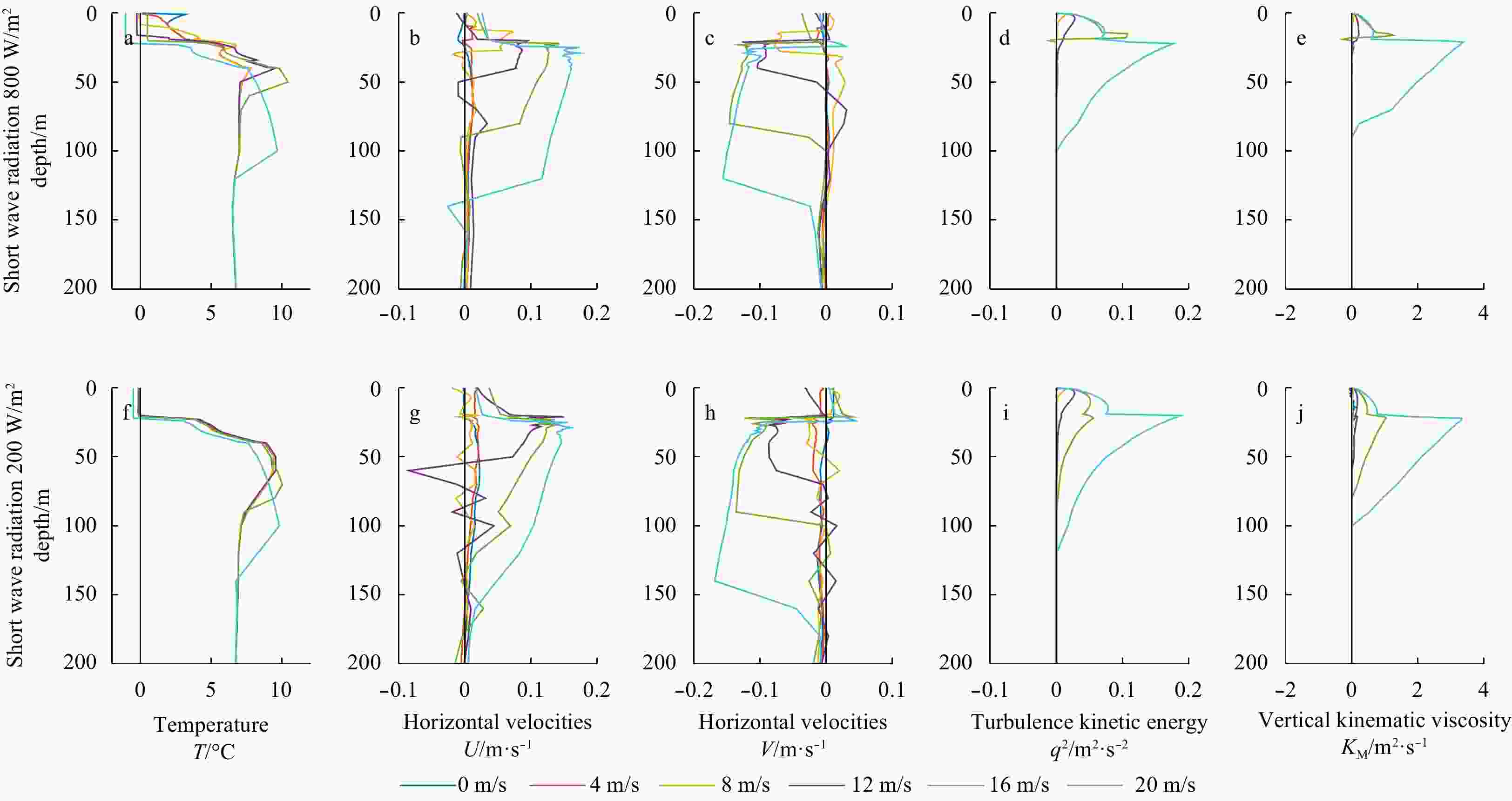
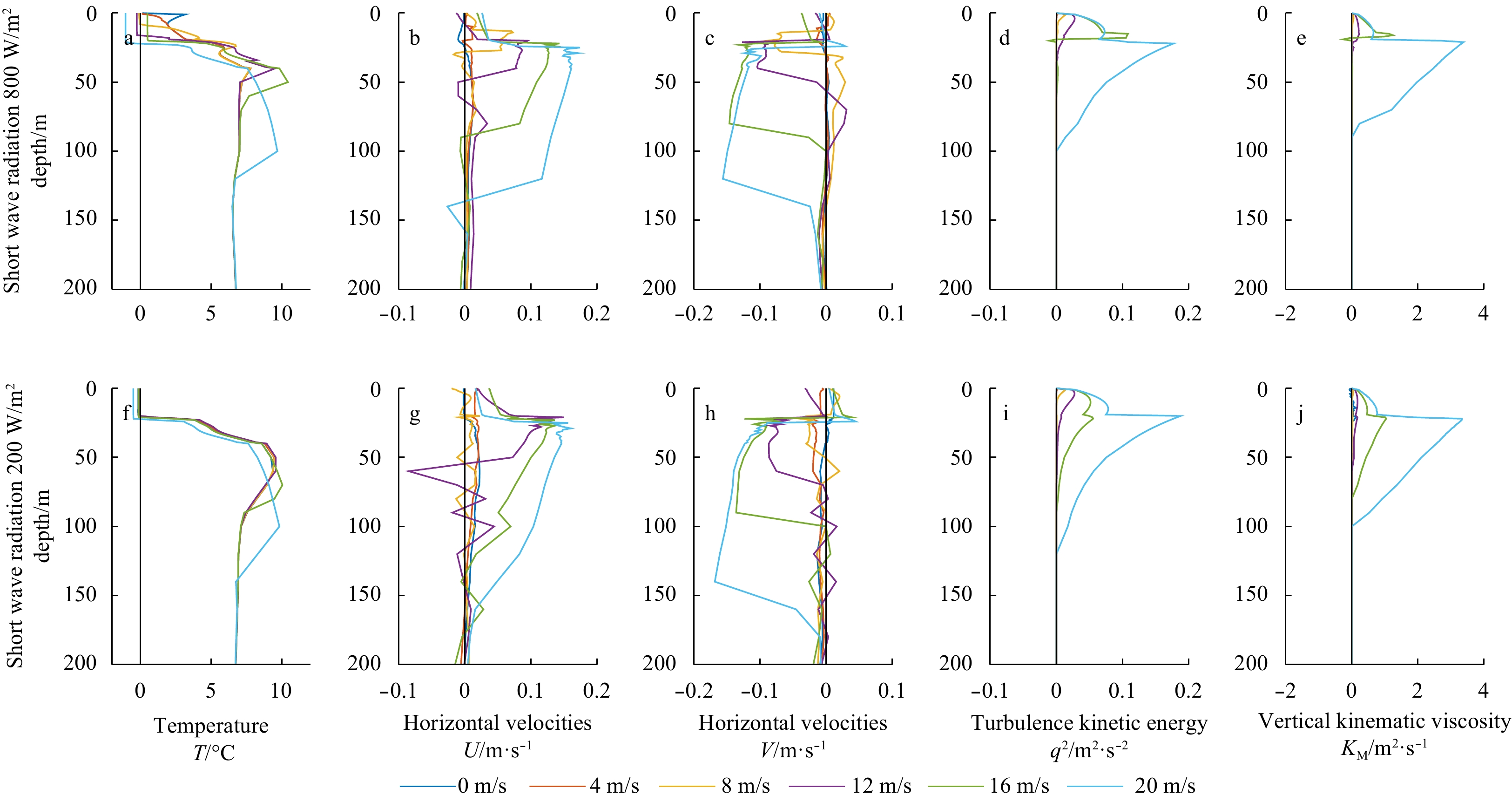
Figure 1. The difference between experiment EXP1-S and EXP1 in the vertical structure of simulated. a, f. Temperature profile (T); b, c, g, h. horizontal velocities (U and V); d, i. turbulence kinetic energy (TKE, q2); and e, j. vertical kinematic viscosity (KM). The colors represent different wind speed, respectively. The top row shows the result forcing by high shortwave radiation 800 W/m2 (a–e), the other row shows that forcing by low short wave radiation 200 W/m2 (f–j).
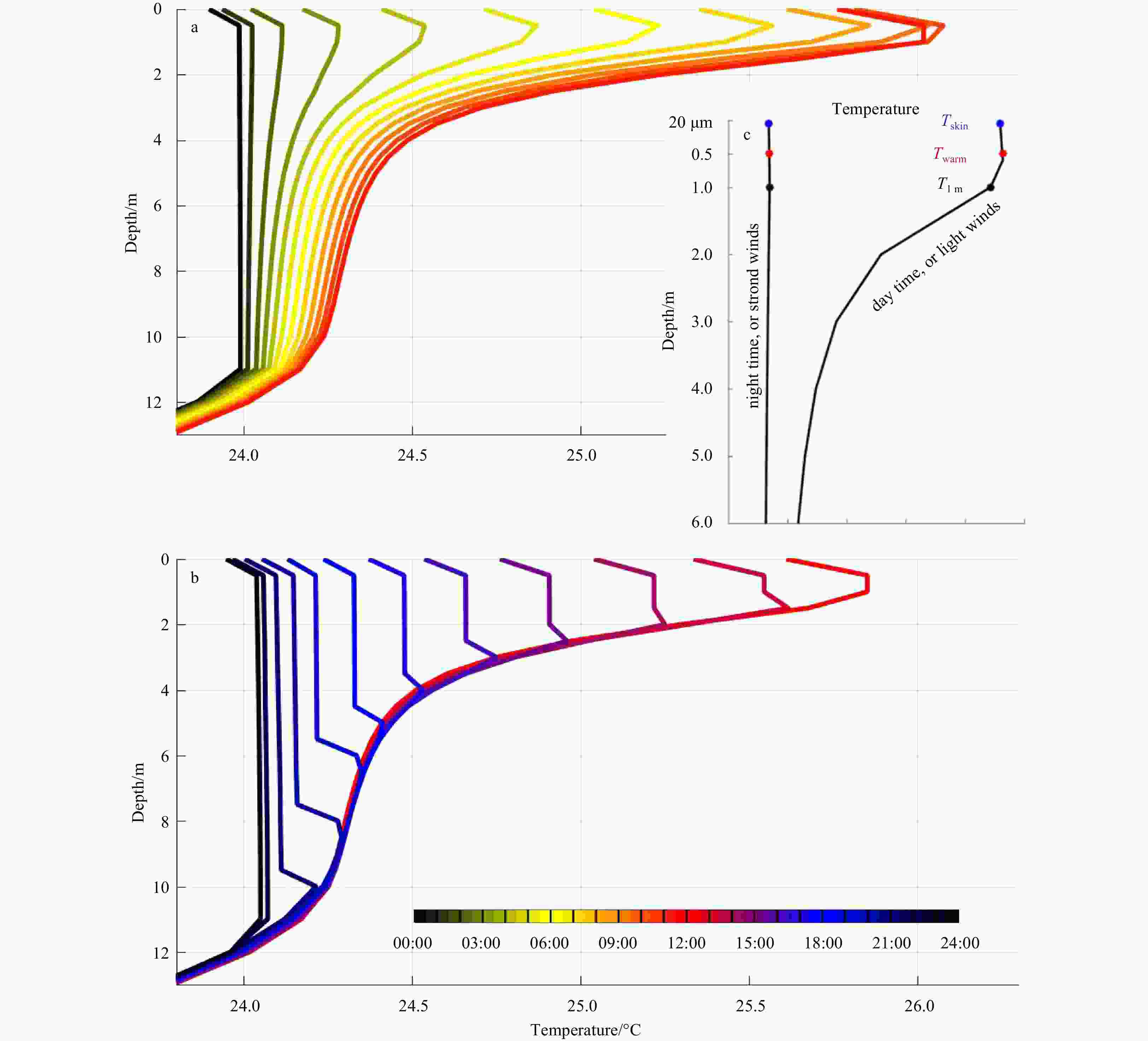
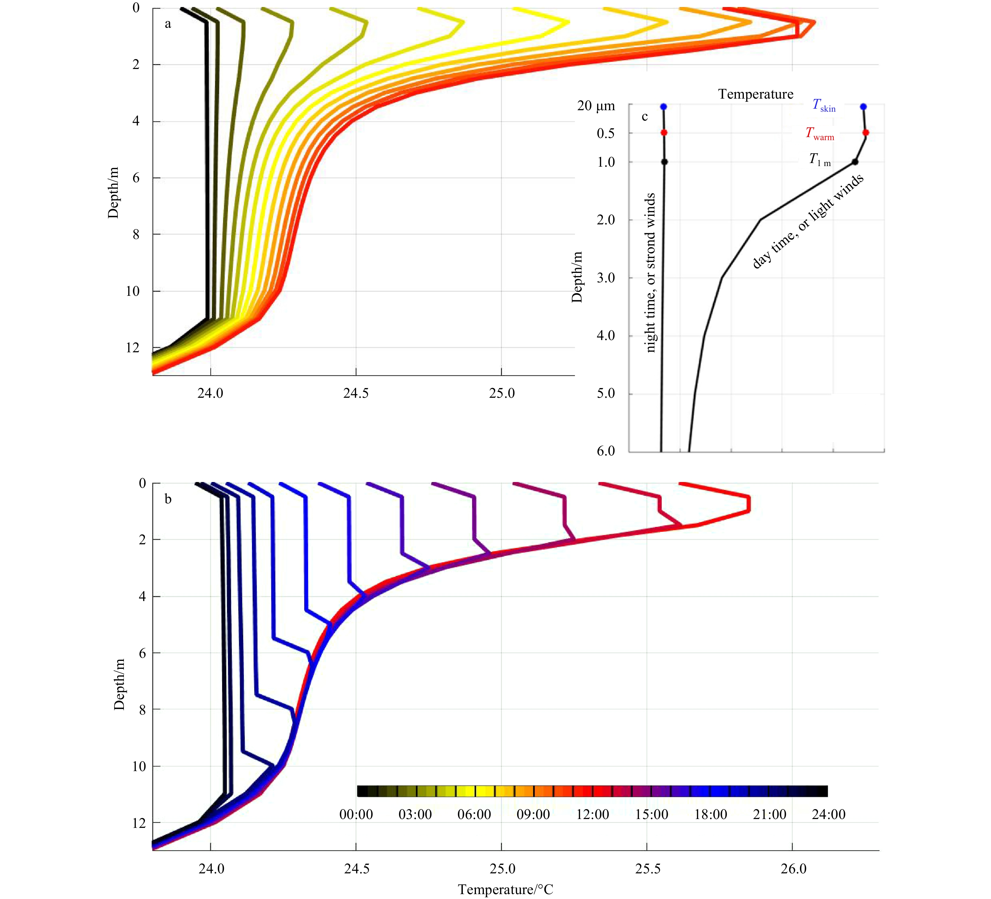
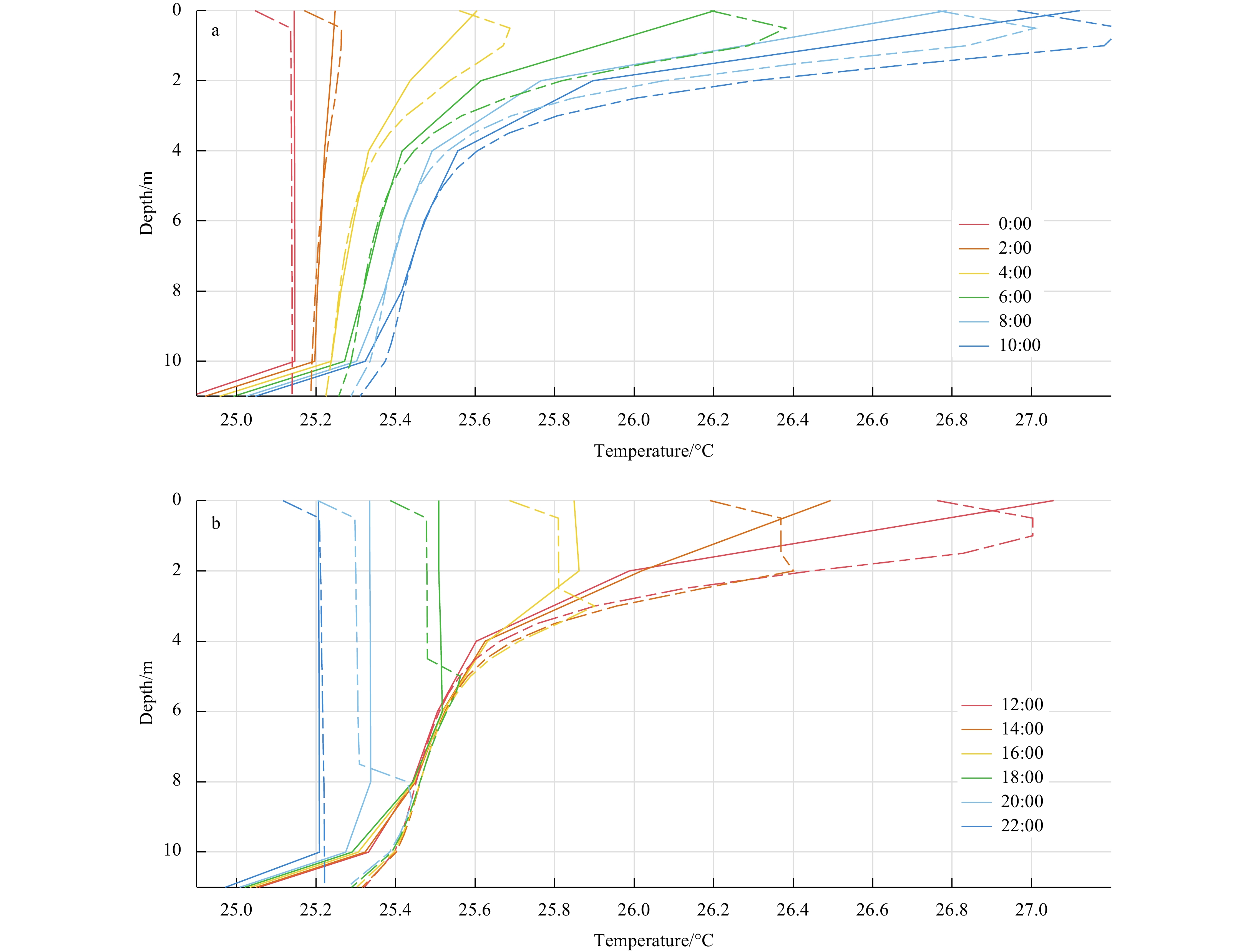
Figure 2. The evolution of sea temperature profile with 2 m/s wind in high vertical resolution model result (EXP2) are shown. The colors represent temperature profile per 1 h, respectively.
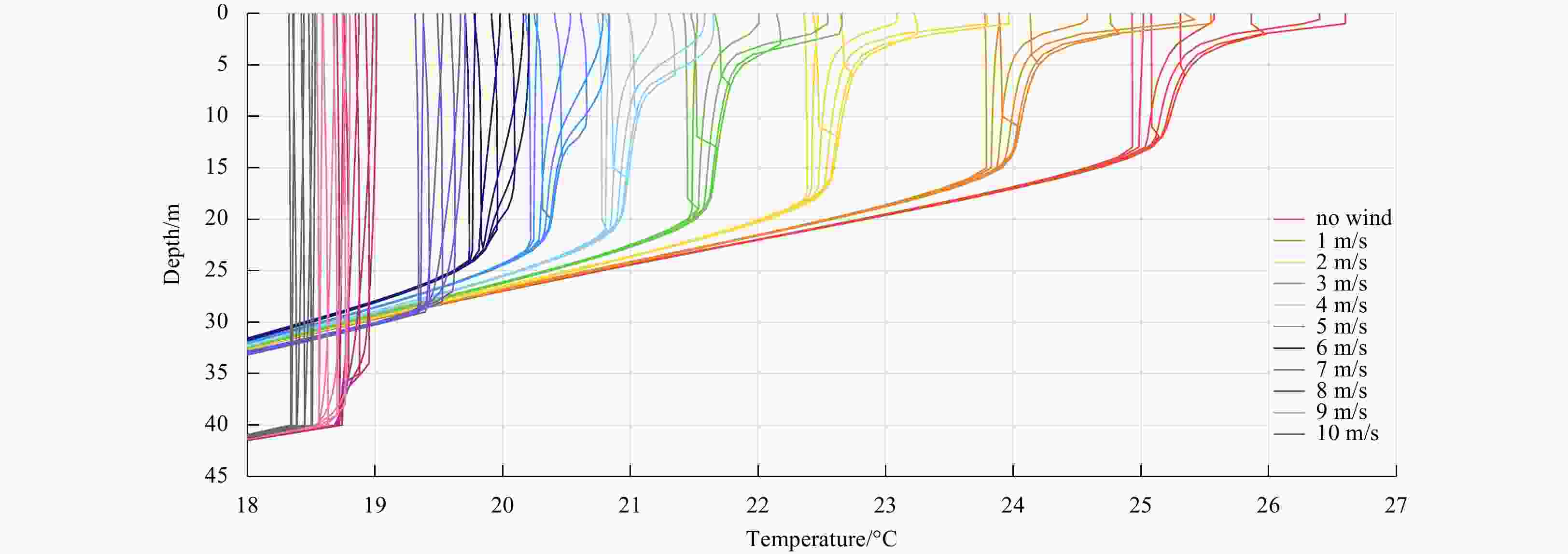
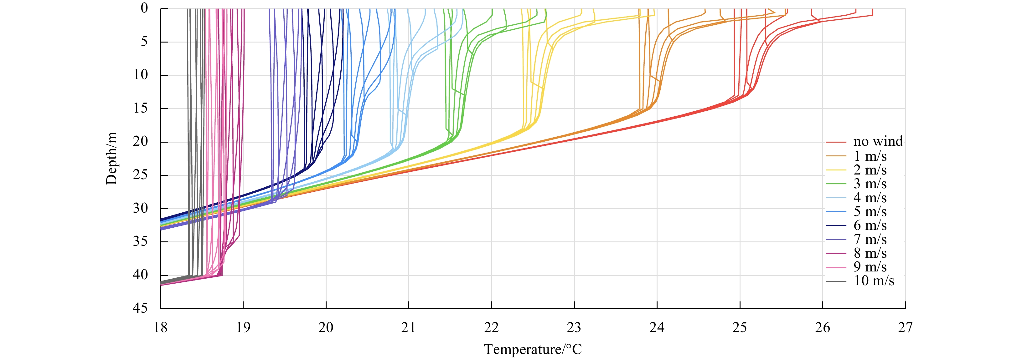
Figure 3. The evolution of sea temperature profile per 3 h in high vertical resolution model result (EXP2) are shown. The colors represent the control experiments with wind speed from 0 to 10 m/s, respectively.

Figure 4. The evolution of sea temperature profile in different control model result. The colors represent temperature profile per 2 h, respectively. Line: EXP1; and line with points: EXP2.
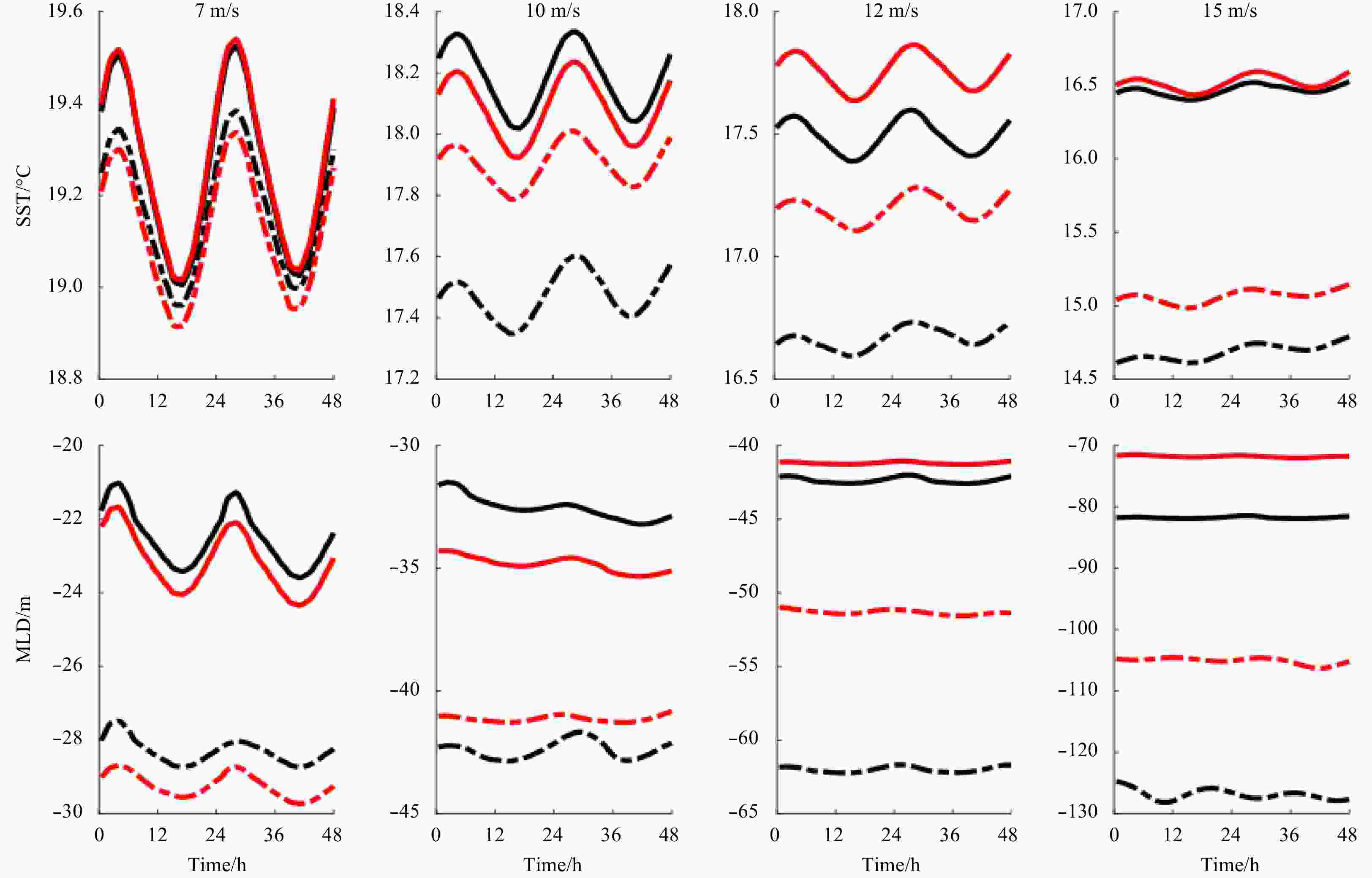
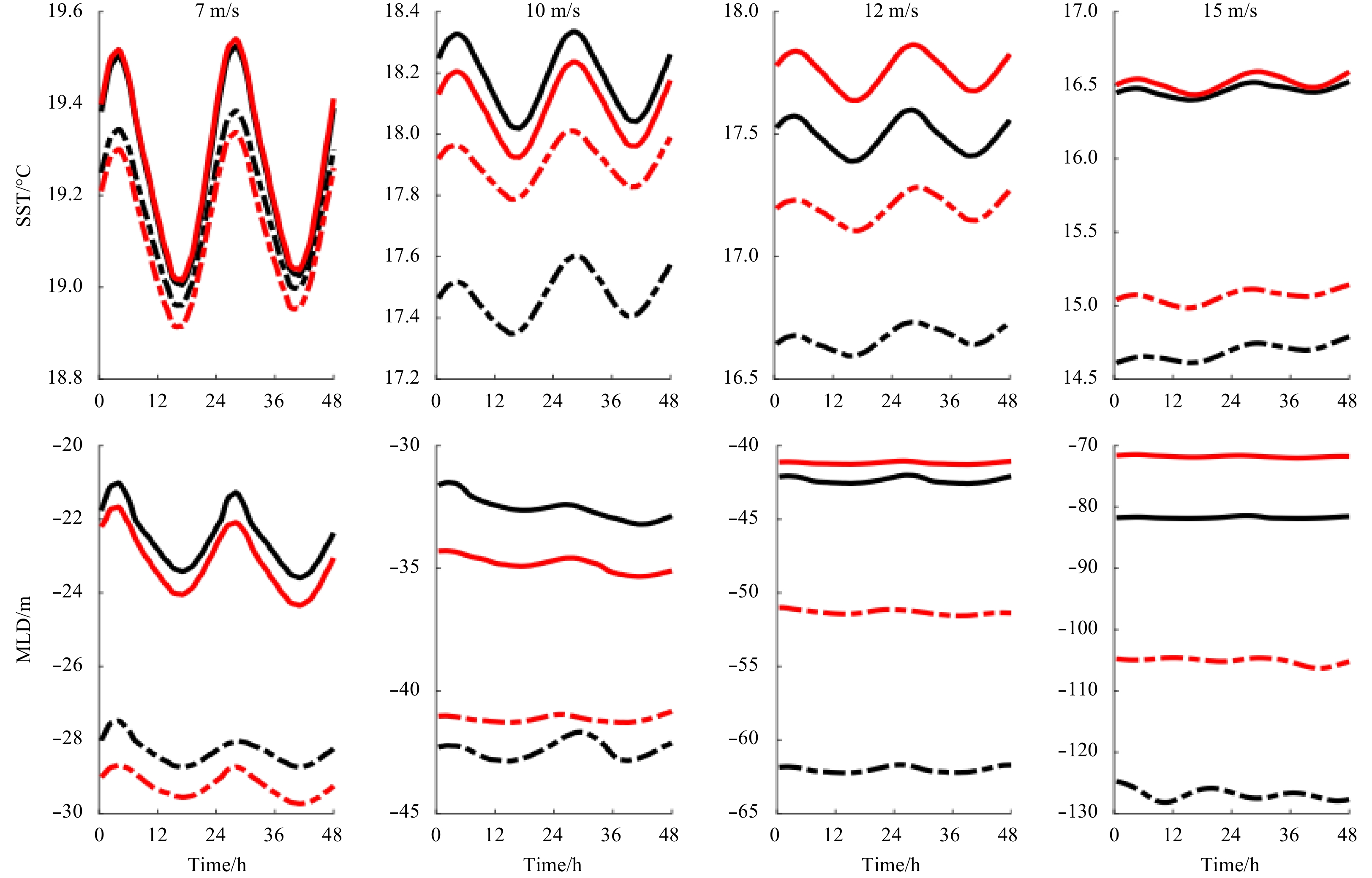
Figure 5. The evolution of MLD and SST in two days with idealized forcing: 800 W/m2 solar radiation and wind speeds from weak to strong. Solid black line: EXP1; solid red line: EXP2; black line with points: EXP1-S; and red line with points: EXP2-S.
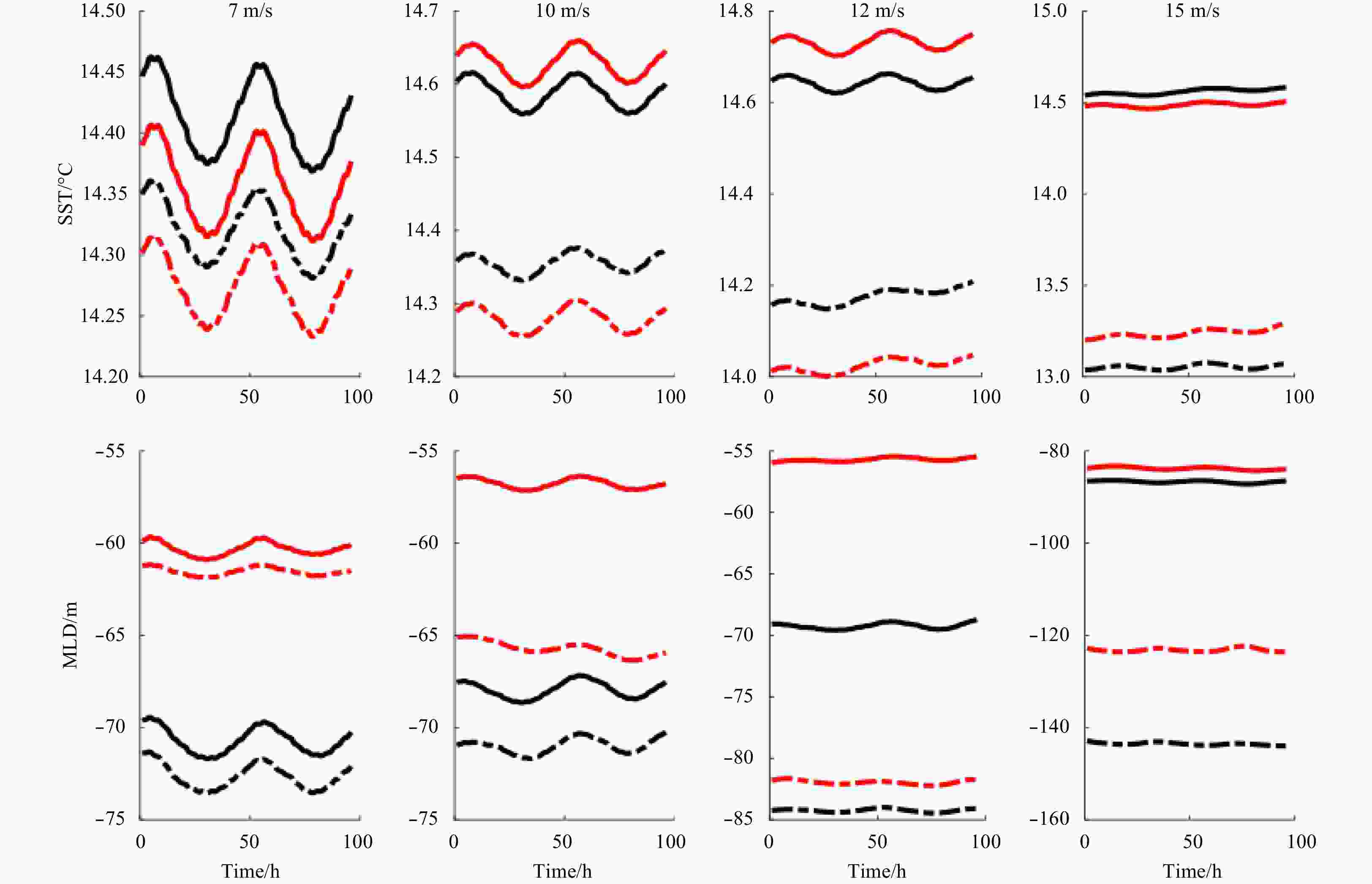
Figure 6. The evolution of MLD and SST in two days with idealized forcing: 200 W/m2 solar radiation and wind speeds from weak to strong. Solid black line: EXP1; solid red line: EXP2; black line with points: EXP1-S; and red line with points: EXP2-S.

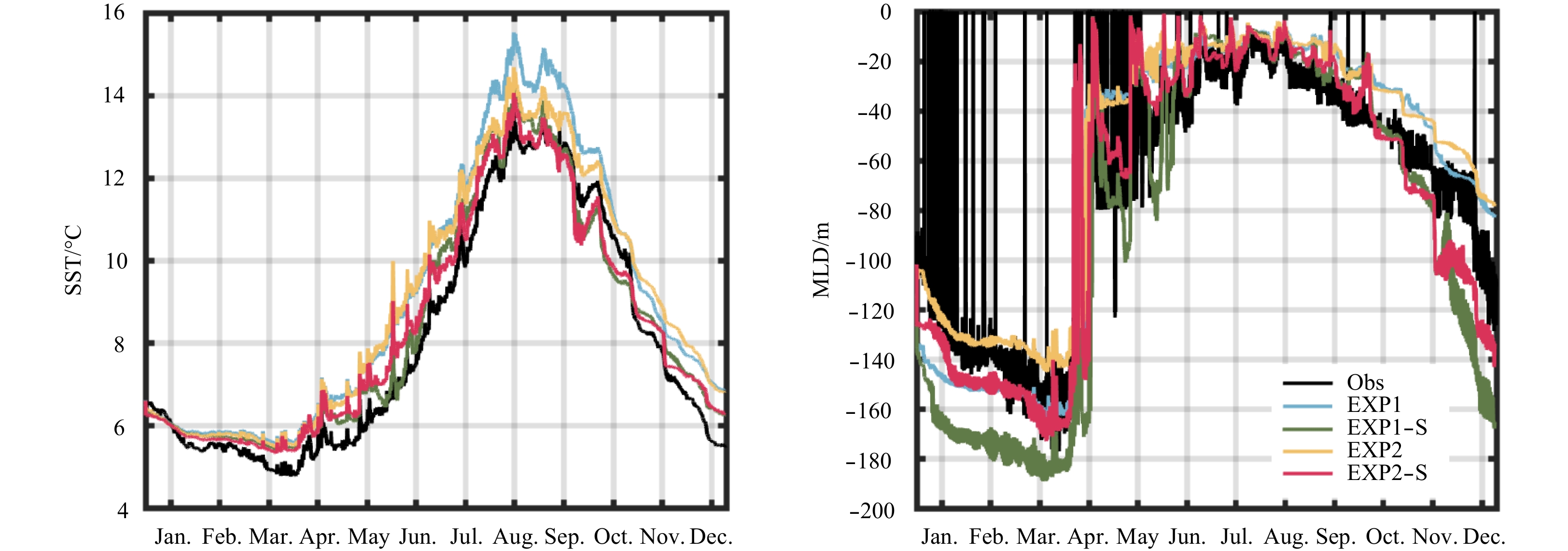
Figure 7. Observed and simulated SST and MLD at Station Papa for 2012. Black line: observation; blue line: EXP1; green line: EXP1-S; yellow line: EXP2; and red line: EXP2-S.
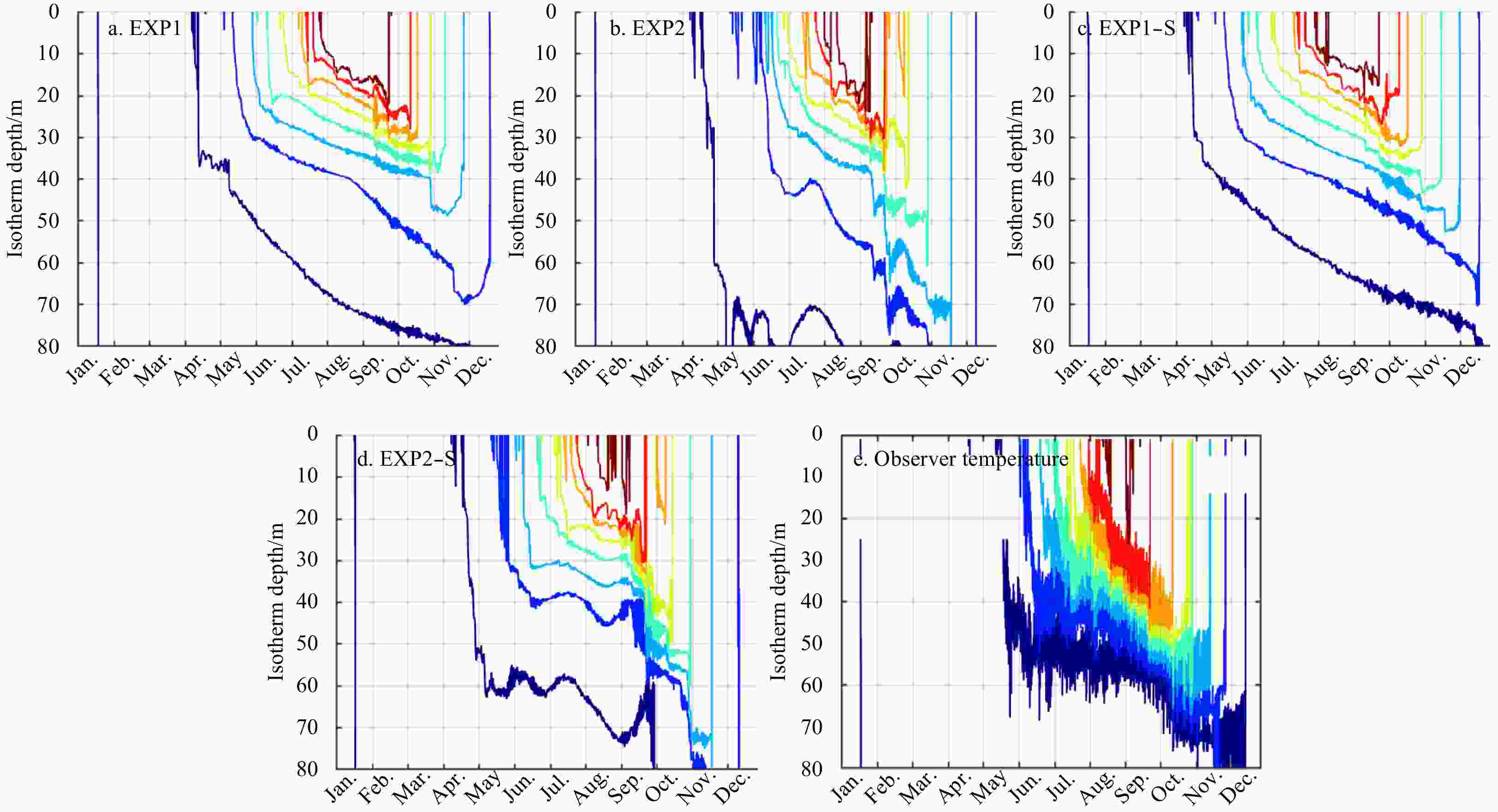
Figure 8. Observed and simulated isotherm depth at Station Papa for 2012. a. EXP1, b. EXP2, c. EXP1-S, d. EXP2-S, and e. observation.

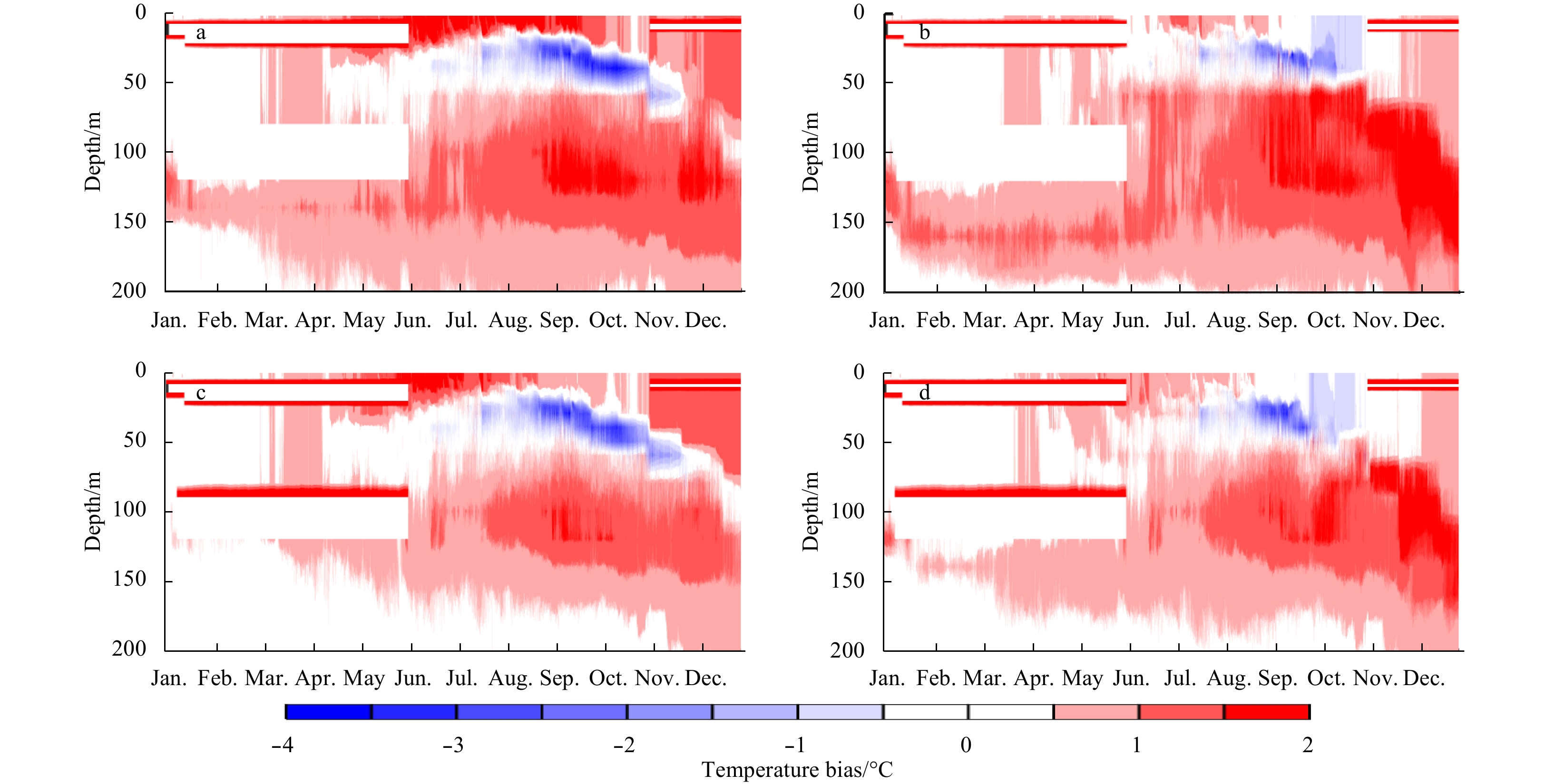
Figure 9. Simulated temperature bias profile at Station Papa for 2012. a. EXP1, b. EXP1-S, c. EXP2, and d. EXP2-S.
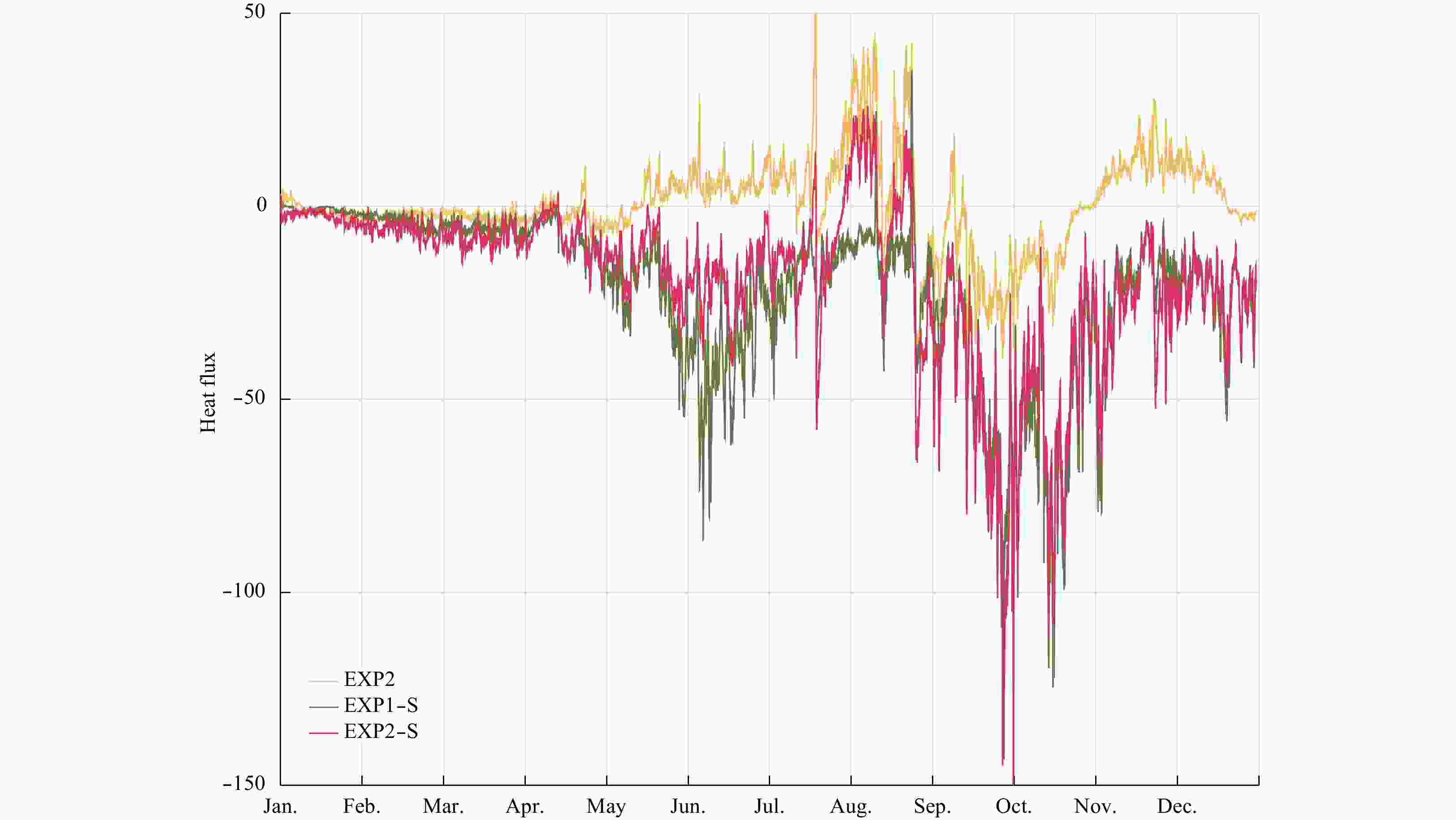
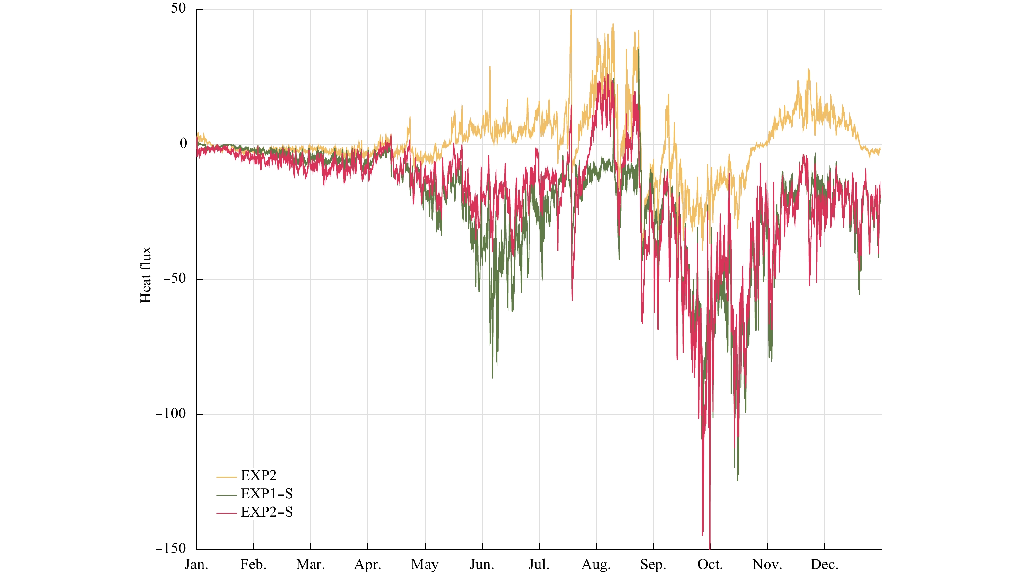
Figure 10. The difference of the net heat flux released into the atmosphere compared with EXP1. Yellow line: EXP2; green line: EXP1-S; and red line: EXP2-S.
Table 1. Summery of the experiments used in this study
Experiment Vertical resolution Stokes drifts Idealized forcing OWS Papa Wind speed
/m·s–1Amplitudes of the solar radiation
/W·m–2Wind speed
/m·s–1Solar radiation
/W·m–2EXP1 low no 0–20 200/800 observed observed EXP2 high no 0–20 200/800 observed observed EXP1-S low yes 0–20 200/800 observed observed EXP2-S high yes 0–20 200/800 observed observed  下载: 导出CSV
Table 2. Difference between model and observed SST and MLD at Papa for 2012
Bias EXP1 EXP2 EXP1-S EXP2-S Annual SST/°C 1.18 0.96 0.57 0.53 Summer SST/°C 1.98 1.21 0.64 0.48 Winter MLD/m 9.03 8.36 28.94 7.65 Summer MLD/m 13.11 12.11 8.05 6.17
下载: 导出CSV
-
[1] Alappattu D P, Wang Qing, Yamaguchi R, et al. 2017. Warm layer and cool skin corrections for bulk water temperature measurements for air-sea interaction studies. Journal of Geophysical Research: Oceans, 122(8): 6470–6481. doi: 10.1002/2017JC012688 [2] Ardhuin F, Jenkins A D. 2006. On the interaction of surface waves and upper ocean turbulence. Journal of Physical Oceanography, 36(3): 551–557. doi: 10.1175/JPO2862.1 [3] Chen Siyu, Qiao Fangli, Huang Chuanjiang, et al. 2018. Effects of the non-breaking surface wave-induced vertical mixing on winter mixed layer depth in subtropical regions. Journal of Geophysical Research: Oceans, 123(4): 2934–2944. doi: 10.1002/2017JC013038 [4] Craig P D, Banner M L. 1994. Modeling wave-enhanced turbulence in the ocean surface layer. Journal of Physical Oceanography, 24(12): 2546–2559. doi: 10.1175/1520-0485(1994)024<2546:MWETIT>2.0.CO;2 [5] Donlon C J, Minnett P J, Gentemann C, et al. 2002. Toward improved validation of satellite sea surface skin temperature measurements for climate research. Journal of Climate, 15(4): 353–369. doi: 10.1175/1520-0442(2002)015<0353:TIVOSS>2.0.CO;2 [6] Fairall C W, Bradley E F, Godfrey J S, et al. 1996a. Cool-skin and warm-layer effects on sea surface temperature. Journal of Geophysical Research: Oceans, 101(C1): 1295–1308. doi: 10.1029/95JC03190 [7] Fairall C W, Bradley E F, Rogers D P, et al. 1996b. Bulk parameterization of air-sea fluxes for tropical ocean-global atmosphere coupled-ocean atmosphere response experiment. Journal of Geophysical Research: Oceans, 101(C2): 3747–3764. doi: 10.1029/95JC03205 [8] Halpern D, Reed R K. 1976. Heat Budget of the Upper Ocean Under Light Winds. Journal of Physical Oceanography, : doi: 10.1175/1520-0485(1976)006<0972:hbotuo>2.0.co;2 [9] Harcourt R R, D’Asaro E A. 2008. Large-eddy simulation of Langmuir turbulence in pure wind seas. Journal of Physical Oceanography, 38(7): 1542–1562. doi: 10.1175/2007JPO3842.1 [10] Huang Chuanjiang, Qiao Fangli, Song Zhenya, et al. 2011. Improving simulations of the upper ocean by inclusion of surface waves in the Mellor-Yamada turbulence scheme. Journal of Geophysical Research: Oceans, 116(C1): C01007. doi: 10.1029/2010JC006320 [11] Kantha L H, Clayson C A. 1994. An improved mixed layer model for geophysical applications. Journal of Geophysical Research: Oceans, 99(C12): 25235–25266. doi: 10.1029/94JC02257 [12] Kantha L H, Clayson C A. 2004. On the effect of surface gravity waves on mixing in the oceanic mixed layer. Ocean Modelling, 6(2): 101–124. doi: 10.1016/S1463-5003(02)00062-8 [13] Kantha L, Tamura H, Miyazawa Y. 2014. Comment on “wave-turbulence interaction and its induced mixing in the upper ocean” by Huang and Qiao. Journal of Geophysical Research: Oceans, 119(2): 1510–1515. doi: 10.1002/2013JC009318 [14] Katsaros K B, Liu W T, Businger J A, et al. 1977. Heat thermal structure in the interfacial boundary layer measured in an open tank of water in turbulent free convection. Journal of Fluid Mechanics, 83(2): 311–335. doi: 10.1017/S0022112077001219 [15] Kenyon K E. 1969. Stokes drift for random gravity waves. Journal of Geophysical Research, 74(28): 6991–6994. doi: 10.1029/JC074i028p06991 [16] Kumar N, Feddersen F. 2017. The effect of stokes drift and transient rip currents on the inner shelf. Part II: With stratification. Journal of Physical Oceanography, 47(1): 243–260. doi: 10.1175/JPO-D-16-0077.1 [17] Martin P J. 1985. Simulation of the mixed layer at OWS November and Papa with several models. Journal of Geophysical Research: Oceans, 90(C1): 903–916. doi: 10.1029/JC090iC01p00903 [18] Matthews A J, Baranowski D B, Heywood K J, et al. 2014. The surface diurnal warm layer in the Indian ocean during CINDY/DYNAMO. Journal of Climate, Special issue: 9101–9122. doi: 10.1175/JCLI-D-14-00222.1 [19] McWilliams J C, Sullivan P P, Moeng C H. 1997. Langmuir turbulence in the ocean. Journal of Fluid Mechanics, 334(1): 1–30. doi: 10.1017/S0022112096004375 [20] Mellor G L. 2001. One-dimensional, ocean surface layer modeling: A problem and a solution. Journal of Physical Oceanography, 31(3): 790–809. doi: 10.1175/1520-0485(2001)031<0790:ODOSLM>2.0.CO;2 [21] Mellor G, Blumberg A. 2004. Wave breaking and ocean surface layer thermal response. Journal of Physical Oceanography, 34(3): 693–698. doi: 10.1175/2517.1 [22] Mellor G L, Yamada T. 1982. Development of a turbulence closure model for geophysical fluid problems. Reviews of Geophysics, 20(4): 851–875. doi: 10.1029/RG020i004p00851 [23] Min H S, Noh Y. 2004. Influence of the surface heating on Langmuir circulation. Journal of Physical Oceanography, 34(12): 2630–2641. doi: 10.1175/JPOJPO-2654.1 [24] Paulson C A, Simpson J J. 1981. The temperature difference across the cool skin of the ocean. Journal of Geophysical Research: Oceans, 86(C11): 11044–11054. doi: 10.1029/jc086ic11p11044 [25] Saunders P M. 1967. The temperature at the ocean-air interface. Journal of the Atmospheric Sciences, 24(3): 269–273. doi: 10.1175/1520-0469(1967)024<0269:ttatoa>2.0.co;2 [26] Smith T A, Chen Sue, Campbell T, et al. 2013. Ocean-wave coupled modeling in COAMPS-TC: A study of Hurricane Ivan (2004). Ocean Modelling, 69: 181–194. doi: 10.1016/j.ocemod.2013.06.003 [27] Soloviev A, Lukas R. 1997. Observation of large diurnal warming events in the near-surface layer of the western equatorial Pacific warm pool. Deep-Sea Research Part I: Oceanographic Research Papers, 44(6): doi: 10.1016/S0967-0637(96)00124-0 [28] Stramma L, Cornillon P, Weller R A, et al. 1986. Large diurnal sea surface temperature variability: Satellite and In Situ Measurements. Journal of Physical Oceanography, : doi: 10.1175/1520-0485(1986)016<0827:ldsstv>2.0.co;2 [29] Sullivan P P, McWilliams J C, Melville W K. 2007. Surface gravity wave effects in the oceanic boundary layer: Large-eddy simulation with vortex force and stochastic breakers. Journal of Fluid Mechanics, 593: 405–452. doi: 10.1017/S002211200700897X [30] Teixeira M A C, Belcher S E. 2002. On the distortion of turbulence by a progressive surface wave. Journal of Fluid Mechanics, 458: 229–267. doi: 10.1017/S0022112002007838 [31] Tseng W L, Tsuang B J, Keenlyside N S, et al. 2015. Resolving the upper-ocean warm layer improves the simulation of the Madden-Julian oscillation. Climate Dynamics, 44(5–6): 1487–1503. doi: 10.1007/s00382-014-2315-1 [32] Tu C Y, Tsuang B J. 2005. Cool-skin simulation by a one-column ocean model. Geophysical Research Letters, 32(22): L22602. doi: 10.1029/2005GL024252 [33] Ward B, Donelan M A. 2006. Thermometric measurements of the molecular sublayer at the air-water interface. Geophysical Research Letters, 33(7): L07605. doi: 10.1029/2005GL024769 [34] Wilson B W. 1965. Numerical prediction of ocean waves in the North Atlantic for December, 1959. Deutsche Hydrografische Zeitschrift, 18(3): 114–130. doi: 10.1007/BF02333333 [35] Wong E W, Minnett P J. 2018. The response of the ocean thermal skin layer to variations in incident infrared radiation. Journal of Geophysical Research: Oceans, 123(4): 2475–2493. doi: 10.1002/2017JC013351 [36] Wu Jin. 1985. On the cool skin of the ocean. Boundary-Layer Meteorology, 31(2): 203–207. doi: 10.1007/BF00121179 [37] Wu Lichuan, Rutgersson A, Sahlée E. 2015. Upper-ocean mixing due to surface gravity waves. Journal of Geophysical Research: Oceans, 120(12): 8210–8228. doi: 10.1002/2015JC011329 [38] Wurl O, Landing W M, Mustaffa N I H, et al. 2019. The ocean’s skin layer in the tropics. Journal of Geophysical Research: Oceans, 124(1): 59–74. doi: 10.1029/2018JC014021 -


 点击查看大图
计量
- 文章访问数: 187
- HTML全文浏览量: 54
- PDF下载量: 3
- 被引次数: 0

