

-
Abstract: With the accelerated warming of the world, the safety and use of Arctic passages is receiving more attention. Predicting visibility in the Arctic has been a hot topic in recent years because of navigation risks and opening of ice-free northern passages. Numerical weather prediction and statistical prediction are two methods for predicting visibility. As microphysical parameterization schemes for visibility are so sophisticated, visibility prediction using numerical weather prediction models includes large uncertainties. With the development of artificial intelligence, statistical prediction methods have received increasing attention. In this study, we constructed a statistical model with a physical basis, to predict visibility in the Arctic based on a dynamic Bayesian network, and tested visibility prediction over a 1°×1° grid area averaged daily. The results show that the mean relative error of the predicted visibility from the dynamic Bayesian network is approximately 14.6% compared with the inferred visibility from the artificial neural network. However, dynamic Bayesian network can predict visibility for only 3 days. Moreover, with an increase in predicted area and period, the uncertainty of the predicted visibility becomes larger. At the same time, the accuracy of the predicted visibility is positively correlated with the time period of the input evidence data. It is concluded that using a dynamic Bayesian network to predict visibility can be useful over Arctic regions for projected climatic changes.
-
Key words:
- Arctic /
- visibility prediction /
- artificial neural network /
- dynamic Bayesian network
-
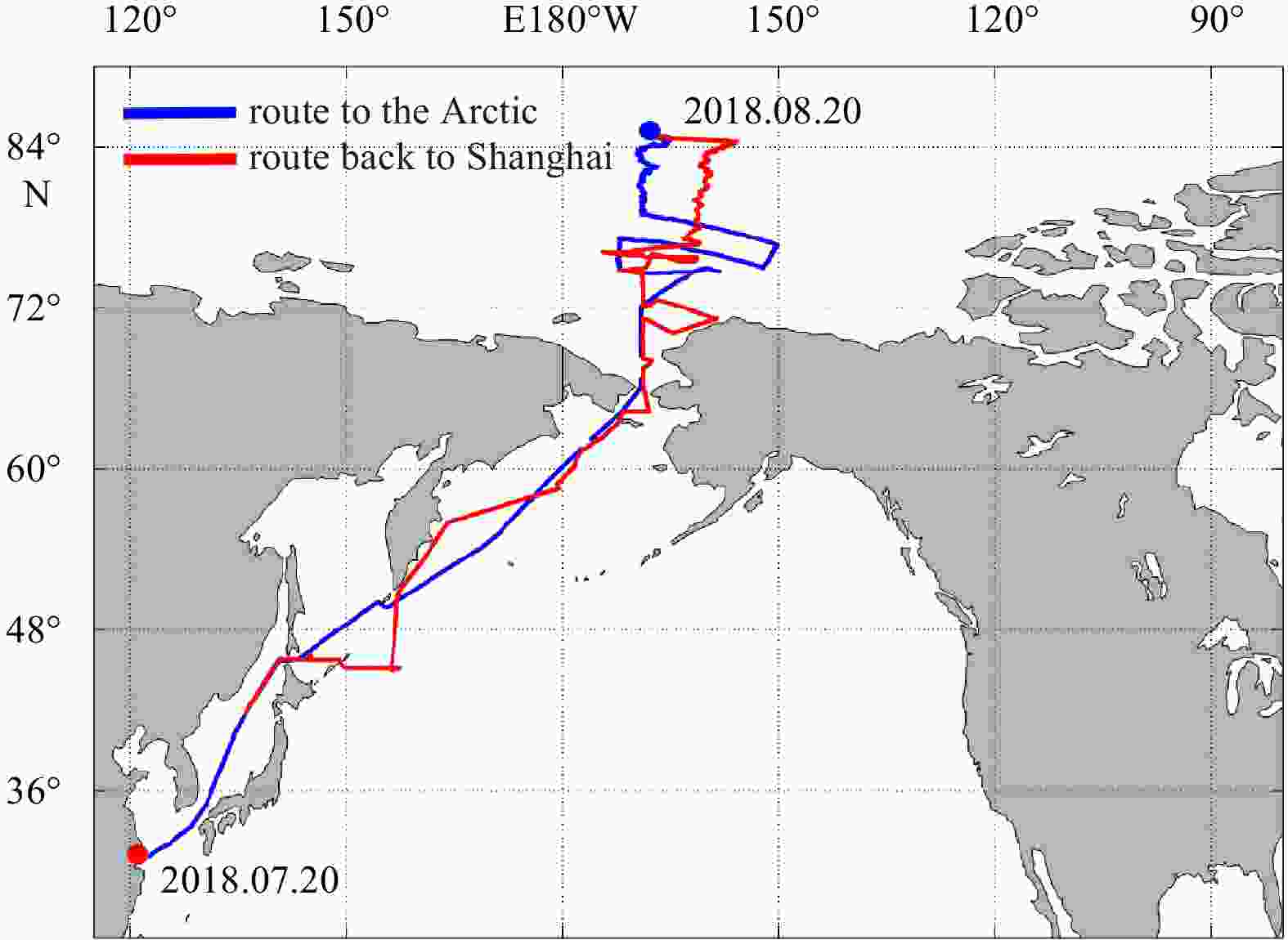
Figure 1. Navigation trajectory of the ice breaker ship used during the Chinese 9th Arctic Science Expedition from July 20 to September 26, 2018.
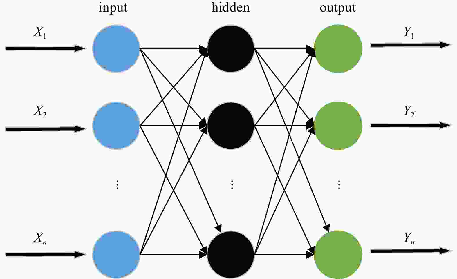
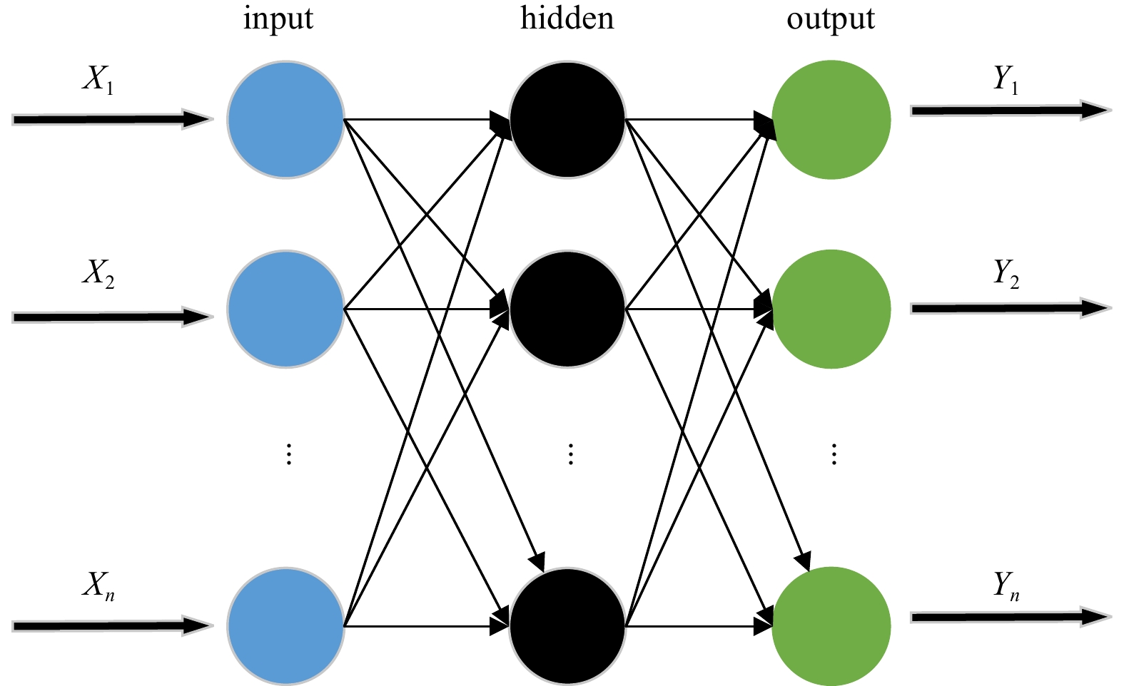
Figure 3. Topological structure of the backpropagation network, which includes only one layer of the hidden layer.
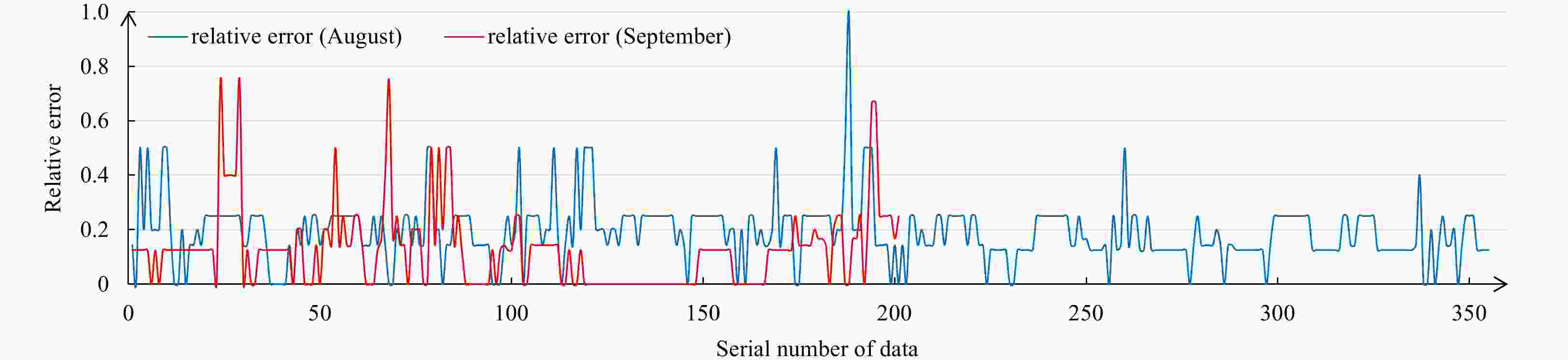
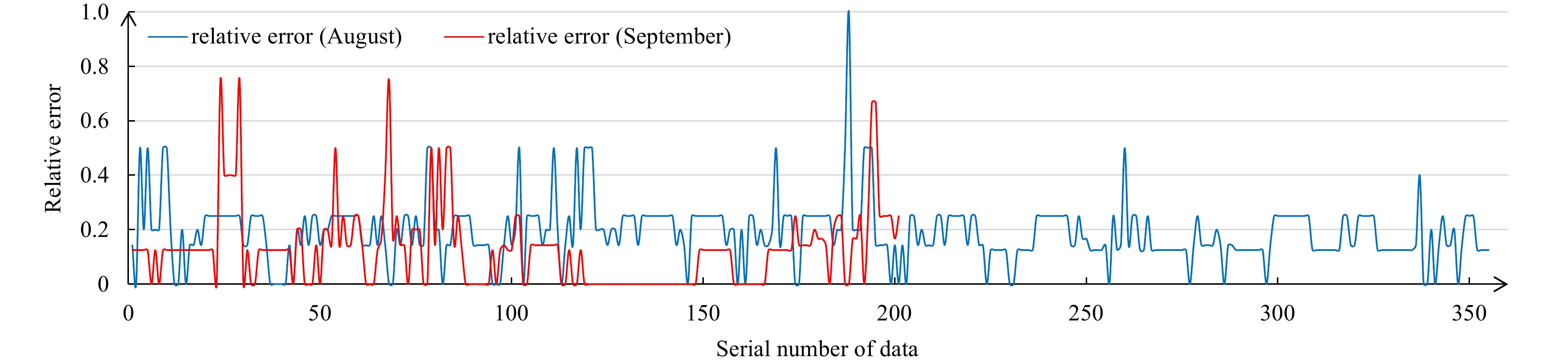
Figure 5. Relative error (δ) of inferred Vis from Eq. (6) against observations obtained from the Chinese 9th Arctic Science Expedition.
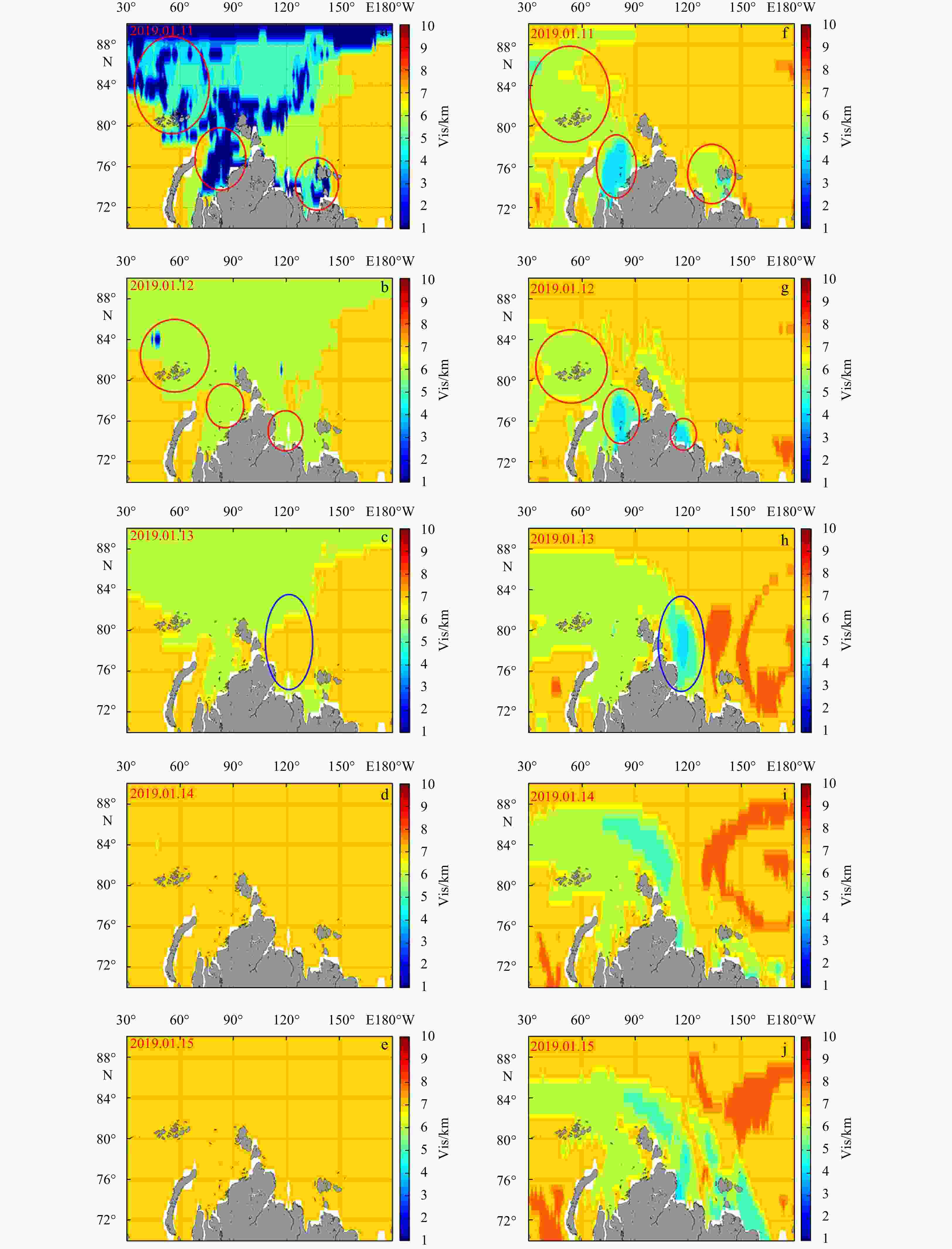
Figure 6. Predicted visibility (Vis) from dynamic Bayesian network and inferred Vis from artificial netural network, for January 11–15, 2019, are shown in boxes a–e and f–j, respectively. The areas with good consistency for the coverage of low Vis between predicted Vis and inferred Vis are marked with red circles, while the areas with bad consistency for this coverage are marked with blue circles.
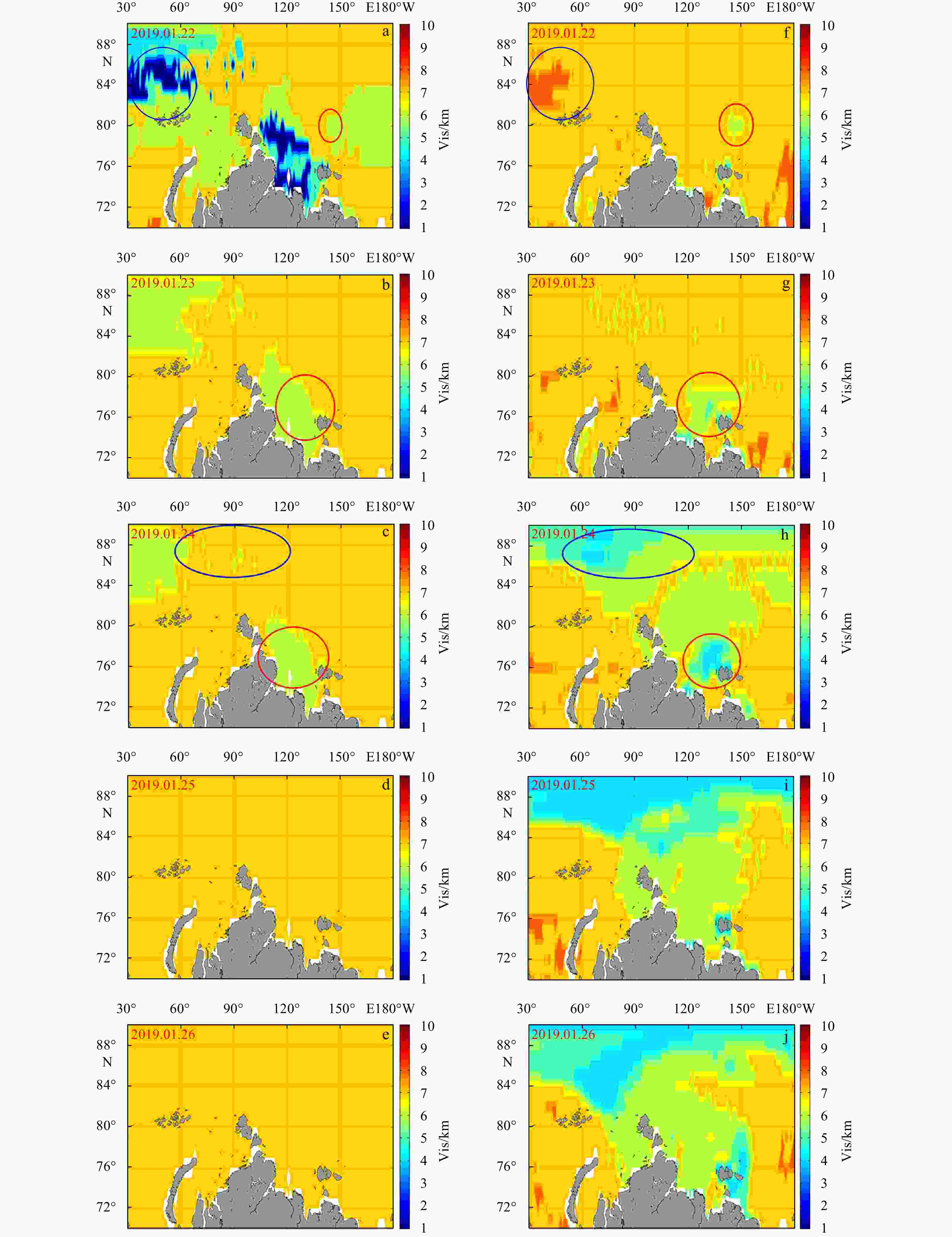
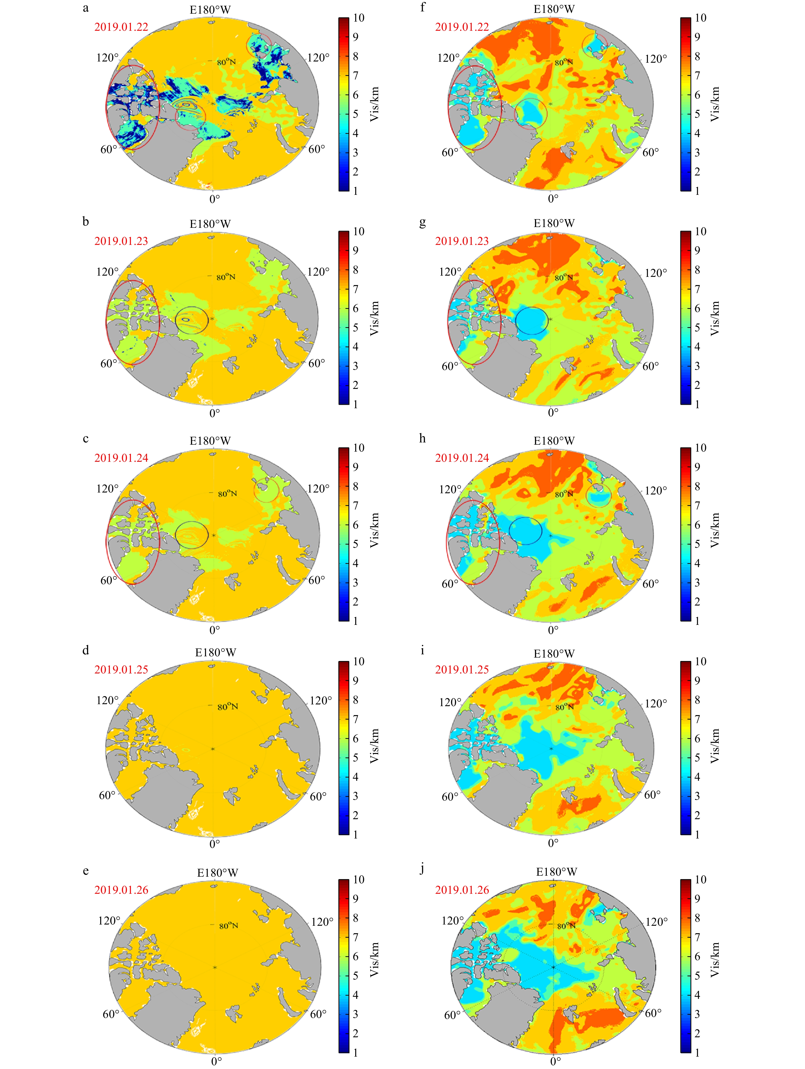
Figure 7. Predicted visibility (Vis) from dynamic Bayesian network and inferred Vis from artificial netural network for January 22–26, 2019, are shown in boxes a–e and f–j, respectively. The areas with good consistency for the coverage of low Vis between the predicted Vis and inferred Vis are marked with red circles, while the areas with bad consistency for this coverage are marked with blue circles.
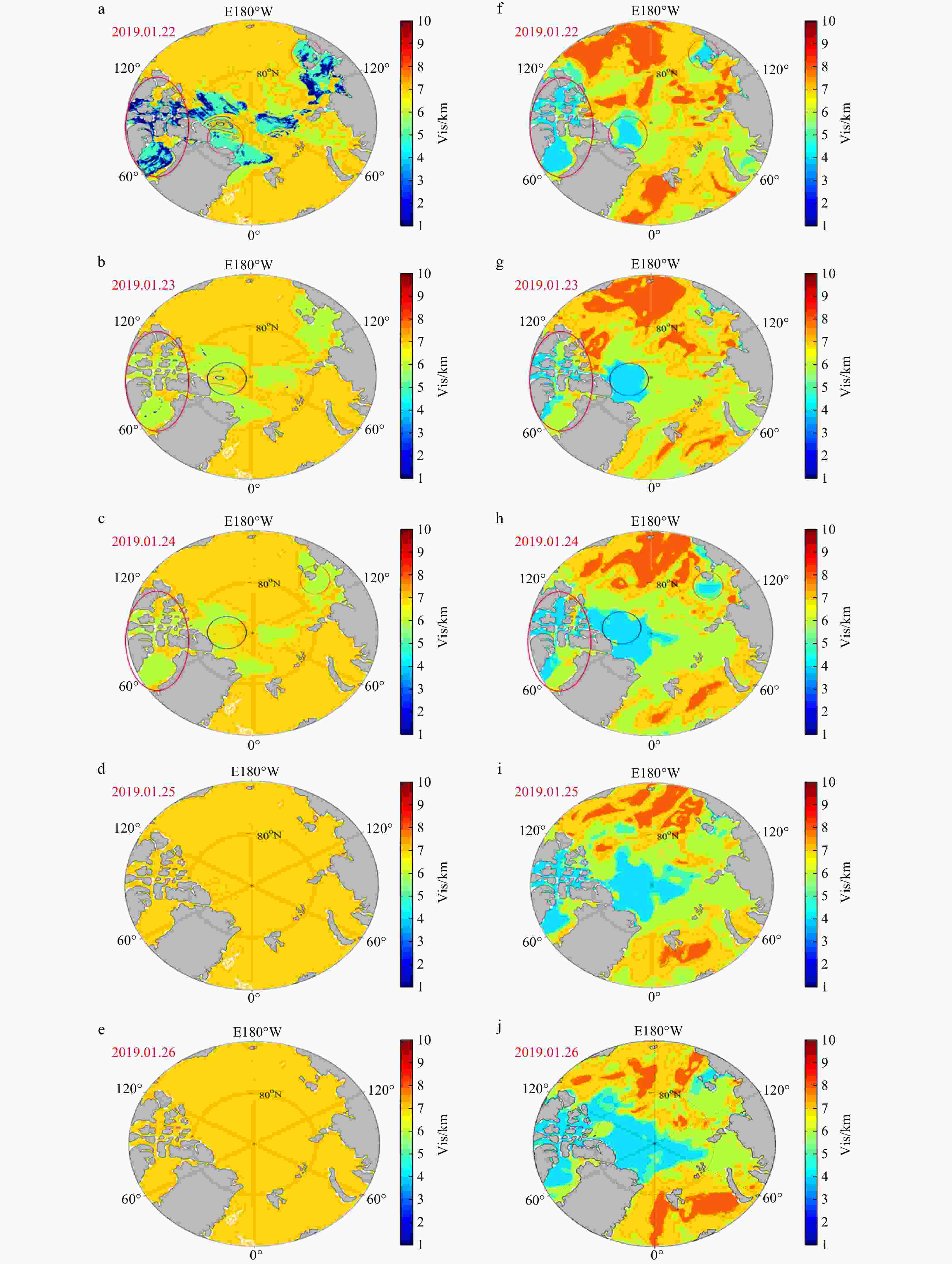
Figure 8. Predicted visibility (Vis) from dynamic Bayesian network and inferred Vis from artificial netural network are shown in boxes a–e and f–j, respectively, for the period of January 22–26, 2019. The areas with good consistency for the coverage of low Vis between the predicted and inferred Vis are marked with red circles, while the areas with bad consistency for this coverage are marked with blue circles.
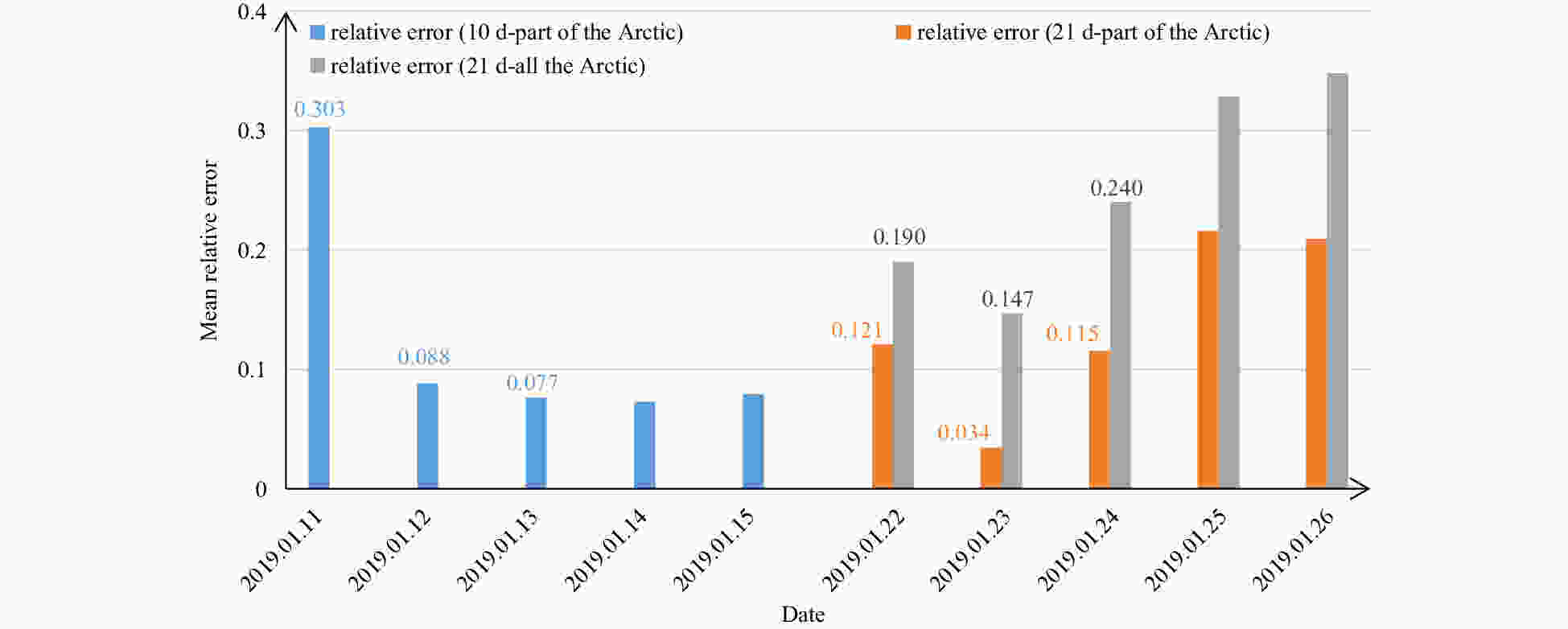
Figure 9. The mean relative error of the daily predicted results relative to the inferred Vis from artificial netural network.
Table 1. Rules of classifying visibility (Vis) levels
Vis level Vis interval/km Vis/km 1 0.05 ≤0.05 2 0.15 0.05–0.20 3 0.3 0.2–0.5 4 0.5 0.5–1.0 5 1 1–2 6 2 2–4 7 6 4–10 8 10 10–20 9 30 20–50 10 − ≥50 Note: − represents no data.  下载: 导出CSV
Table 2. Quality flag (QF) of data records from the International Comprehensive Ocean-Atmosphere Data Set
QF Description of QF 0 no quality control performed 1 element appears correct 2 element appears inconsistent with other elements 3 element appears doubtful 4 element appears erroneous 5 element changed (possibly to missing) as a result of quality control 6 element flagged by contributing member (CM) as correct but according to minimum quality control standard (MQCS) still appears suspect or missing 7 element flagged by CM as changed, but according to MQCS still appears suspect 8 reserved 9 element is missing
下载: 导出CSV
Table 3. Summary of automatic learning methods used in dynamic Bayesian network
The known of structure The integrity of sample data Automatic learning methods known complete simple statistical method known incomplete EM method or gradient descent method unknown complete searching model space unknown incomplete structural EM method
下载: 导出CSV
Table 4. Number of data points for each month in the Arctic obtained from the Chinese 9th Arctic Science Expedition archive
July August September Amount 73 355 201
下载: 导出CSV
Table 5. State transition probability matrix of the trained dynamic Bayesian network, where 1–10 represent the Vis level (state)
Vis 1 2 3 4 5 6 7 8 9 10 1 0.330 0.221 0.167 0.143 0.072 0.034 0.032 0.000 0.000 0.000 2 0.297 0.175 0.118 0.143 0.145 0.055 0.060 0.007 0.000 0.000 3 0.144 0.107 0.133 0.197 0.175 0.176 0.051 0.017 0.000 0.000 4 0.010 0.014 0.029 0.267 0.315 0.270 0.078 0.016 0.000 0.000 5 0.001 0.001 0.004 0.036 0.351 0.434 0.153 0.018 0.000 0.000 6 0.000 0.000 0.001 0.006 0.075 0.564 0.331 0.023 0.000 0.000 7 0.000 0.000 0.000 0.001 0.012 0.137 0.791 0.057 0.001 0.000 8 0.000 0.000 0.000 0.001 0.013 0.091 0.423 0.459 0.012 0.001 9 0.000 0.000 0.000 0.000 0.003 0.062 0.320 0.325 0.277 0.012 10 0.000 0.000 0.001 0.003 0.003 0.257 0.140 0.188 0.288 0.121
下载: 导出CSV
Table 6. Daily prediction success rate of the three prediction experiments
Day 1 Day 2 Day 3 Day 4 Day 5 Average of the
first 3 daysExperiment 1 33.1% 51.4% 55.6% 58.5% 58.7% 46.7% Experiment 2 59.8% 73.9% 46.9% 42.3% 38.1% 60.2% Experiment 3 33.8% 42.8% 29.9% 23.2% 27.5% 35.5%
下载: 导出CSV
-
[1] Boneh T, Weymouth G T, Newham P, et al. 2015. Fog forecasting for Melbourne Airport using a Bayesian decision network. Weather and Forecasting, 30(5): 1218–1233. doi: 10.1175/WAF-D-15-0005.1 [2] Bremnes J B, Michaelides S C. 2007. Probabilistic visibility forecasting using neural networks. Pure and Applied Geophysics, 164(6): 1365–1381. doi: 10.1007/s00024-007-0223-6 [3] Chmielecki R M, Raftery A E. 2011. Probabilistic visibility forecasting using Bayesian model averaging. Monthly Weather Review, 139(5): 1626–1636. doi: 10.1175/2010MWR3516.1 [4] Dee D P, Uppala S M, Simmons A J, et al. 2011. The ERA-Interim reanalysis: Configuration and performance of the data assimilation system. Quarterly Journal of the Royal Meteorological Society, 137(656): 553–597. doi: 10.1002/qj.828 [5] Freeman E, Woodruff S D, Worley S J, et al. 2017. ICOADS Release 3.0: a major update to the historical marine climate record. International Journal of Climatology, 37(5): 2211–2232. doi: 10.1002/joc.4775 [6] Gultepe I, Isaac G A. 2006. Visibility versus precipitation rate and relative humidity. In: 12th Conference on Cloud Physics. Madison, WI: American Meteorological Society, 2: 1161–1178 [7] Gultepe I, Isaac G A, Rasmussen R, et al. 2011. A freezing fog/drizzle event during the FRAM-S project. In: SAE International/AIAA, International Conference on Aircraft and Engine and Ground-De-Icing. Chicago: SAE [8] Gultepe I, Milbrandt J A, Zhou Binbin. 2017. Marine fog: A review on microphysics and visibility prediction. In: Koračin D, Dorman C, eds. Marine Fog: Challenges and Advancements in Observations. Cham: Springer, 345–394 [9] Gultepe I, Müller M D, Boybeyi Z. 2006. A new visibility parameterization for warm-fog applications in numerical weather prediction models. Journal of Applied Meteorology and Climatology, 45(11): 1469–1480. doi: 10.1175/JAM2423.1 [10] Gultepe I, Pavolonis M, Zhou Binbin, et al. 2015. Freezing fog and drizzle observations. In: SAE 2015 International Conference on Icing of Aircraft, Engines, and Structures. Prague, Czech Republic: SAE, [11] Gultepe J, Pearson G, Milbrandt J A, et al. 2009. The fog remote sensing and modeling field project. Bulletin of the American Meteorological Society, 90(3): 341–360. doi: 10.1175/2008BAMS2354.1 [12] Gultepe I, Sharman R, Williams P D, et al. 2019. A review of high impact weather for aviation meteorology. Pure and Applied Geophysics, 176(5): 1869–1921. doi: 10.1007/s00024-019-02168-6 [13] Hong Quan. 2003. The trend of visibility and its affecting factors in Chongqing. Journal of Chongqing University, 26(5): 151–154. doi: 10.3969/j.issn.1000-582X.2003.05.037 [14] Jin W, Li Z J, Wei L S, et al. 2000. The improvements of BP neural network learning algorithm. In: 2000 5th International Conference on Signal Processing Proceedings, 16th World Computer Congress 2000. Piscataway, NJ: IEEE,1647–1649 [15] Kutiel H, Hirsch-Eshkol T R, Türkeş M. 2001. Sea level pressure patterns associated with dry or wet monthly rainfall conditions in Turkey. Theoretical and Applied Climatology, 69(1−2): 39–67. doi: 10.1007/s007040170034 [16] Li Ming, Liu Kefeng. 2018. Application of intelligent dynamic Bayesian network with wavelet analysis for probabilistic prediction of storm track intensity index. Atmosphere, 9(6): 224. doi: 10.3390/atmos9060224 [17] Li Hongxi, Zheng Zhongyi, Li Meng. 2011. A method based on rough sets to assess significance of factors influencing navigation safety in harbor waters. In: 11th International Conference of Chinese Transportation Professionals (ICCTP). Nanjing: American Society of Civil Engineers [18] Marzban C, Leyton S, Colman B. 2007. Ceiling and visibility forecasts via neural networks. Weather and Forecasting, 22(3): 466–479. doi: 10.1175/WAF994.1 [19] McClelland J L, Rumelhart D E, PDP Research Group. 1987. Parallel Distributed Processing, vol. 2: Psychological and Biological Models. Cambridge: A Bradford Book [20] Otto H, Jukka J, Vesa N. 2007. Climatological tools for low visibility forecasting. Pure and Applied Geophysics, 164(6−7): 1383–1396. doi: 10.1007/s00024-007-0224-5 [21] Pasini A, Pelino V, Potestà S. 2001. A neural network model for visibility nowcasting from surface observations: Results and sensitivity to physical input variables. Journal of Geophysical Research: Atmospheres, 106(D14): 14951–14959. doi: 10.1029/2001JD900134 [22] Pearl J. 1988. Probabilistic Reasoning in Intelligent Systems: Networks of Plausible Inference. San Mateo: Morgan Kaufmann Publishers [23] Qu Ping, Xie Yiyang, Liu Lili, et al. 2014. Character Analysis of Sea Fog in Bohai Bay from 1 to 2010. Plateau Meteorology, 33(1): 285–293 [24] Roquelaure S, Bergot T. 2008. A local ensemble prediction system for fog and low clouds: Construction, Bayesian model averaging calibration, and validation. Journal of Applied Meteorology and Climatology, 47(12): 3072–3088. doi: 10.1175/2008JAMC1783.1 [25] Roquelaure S, Bergot T. 2009. Contributions from a Local Ensemble Prediction System (LEPS) for improving fog and low cloud forecasts at airports. Weather and Forecasting, 24(1): 39–52. doi: 10.1175/2008waf2222124.1 [26] Roquelaure S, Tardif R, Remy S, et al. 2009. Skill of a ceiling and visibility local ensemble prediction system (LEPS) according to fog-type prediction at Paris-Charles de Gaulle Airport. Weather and Forecasting, 24(6): 1511–1523. doi: 10.1175/2009WAF2222213.1 [27] Shan Yulong, Zhang Ren, Li Ming, et al. 2019. Generation and analysis of gridded visibility data in the Arctic. Atmosphere, 10(6): 314. doi: 10.3390/atmos10060314 [28] Shi Zhifu, Zhang An. 2012. Bayesian Network Theory and Its Application in Military System. Beijing: National Defense Industry Press, 110 [29] Xu Chenfeng. 2016. Visibility change and applicable rules of action for ships. World Shipping, 39(1): 35–37 [30] Xue Dan, Li Chengfan, Liu Qian. 2015. Visibility characteristics and the impacts of air pollutants and meteorological conditions over Shanghai, China. Environmental Monitoring and Assessment, 187(6): 363. doi: 10.1007/s10661-015-4581-8 [31] Zhao Ping, Zhu Yani, Zhang Qin. 2012. A summer weather index in the East Asian pressure field and associated atmospheric circulation and rainfall. International Journal of Climatology, 32(3): 375–386. doi: 10.1002/joc.2276 [32] Zhou Binbin, Du Jun, Gultepe I, et al. 2012. Forecast of low visibility and fog from NCEP: Current status and efforts. Pure and Applied Geophysics, 169(5-6): 895–909. doi: 10.1007/s00024-011-0327-x -
 supplement-zhaoshijun.pdf

-


 点击查看大图

计量
- 文章访问数: 361
- HTML全文浏览量: 106
- PDF下载量: 13
- 被引次数: 0

