

Temporal and spatial distribution characteristics of nutrients in Clarion-Clipperton Fracture Zone in the Pacific in 2017
-
Abstract: This research investigated eight stations in Clarion-Clipperton Fracture Zone (CCFZ) in the eastern tropical Pacific in 2017 to study the spatial distribution characteristics of nutrients and chlorophyll a (Chl a) concentration, and compared nutrient concentrations and molar ratios with those of other investigations 20 years ago in the same area. The study found that dissolved inorganic nutrient (N, P and Si) concentrations were lowest in the upper layer, and increased from surface to some depths, then they decreased a little to the bottom. N was the limited nutrient factor for the growth of phytoplankton community. Although nutrient concentrations and molar ratios have no obvious changes in 2017 comparing those in 1998−2003, supplemented from the equatorial Pacific, nutrient concentrations in the study area were higher than those in seamounts in the North Pacific and Station ALOHA. Furthermore, this study used Generalized Additive Models (GAMs) to infer the underlying bottom-up factors controlling phytoplankton abundance (Chl a concentration), showing that depth, salinity and
${\rm{PO}}_4^{3 - }{\text -}{\rm{ P}} $ concentration were major factors controlling the growth of phytoplankton community. Furthermore, this study can provide basic data and theoretical support for the development of polymetallic nodule area and its long-term impact assessment on the environment. -

Figure 1. Map of the investigation area in CCFZ. The triangle represents the location of stations in seamounts of the subtropical western Pacific Ocean, the circle represents Station ALOHA.

Figure 2. Sectional distribution of temperature and salinity in CCFZ. These stations from left to right were the eight investigated stations from the south to the north, named CC-S01, KW1-S37, KW1-S05, KW1-S40, KW1-S01, CC-S10, CC-S09, CC-S06. These black dots are sampling sites.

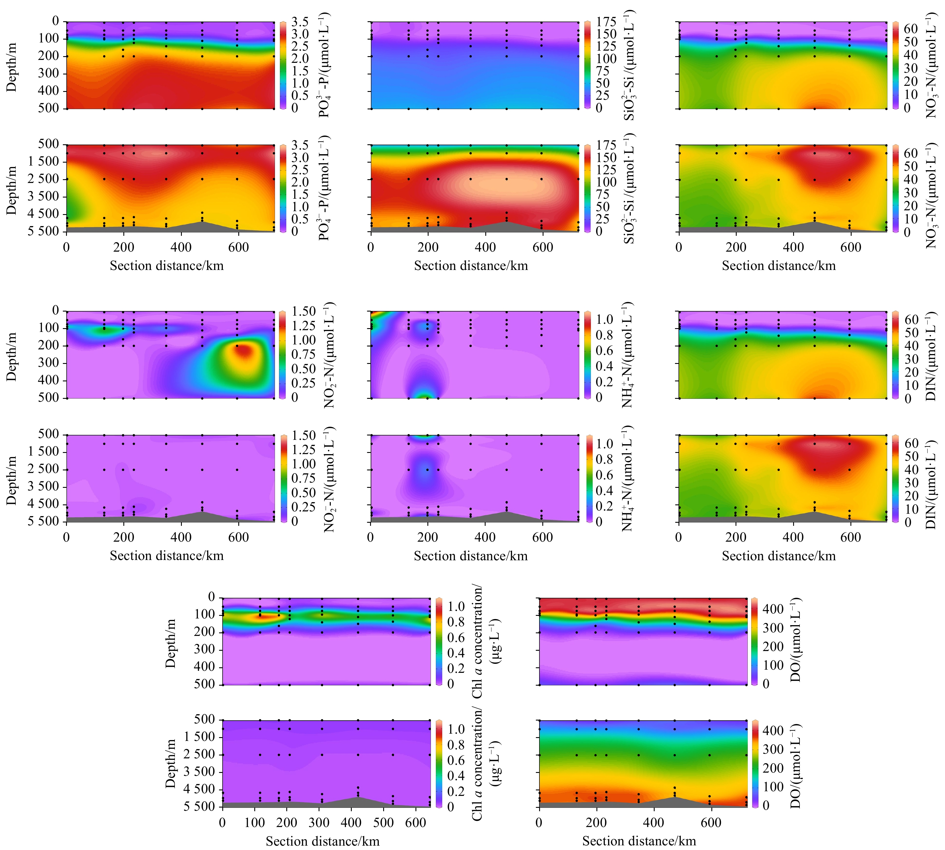
Figure 4. Sectional distribution of nutrients, DO and Chl a concentration in CCFZ. These stations from left to right were the eight investigated stations from the south to the north, named CC-S01, KW1-S37, KW1-S05, KW1-S40, KW1-S01, CC-S10, CC-S09, CC-S06. These black dots aresampling sites.

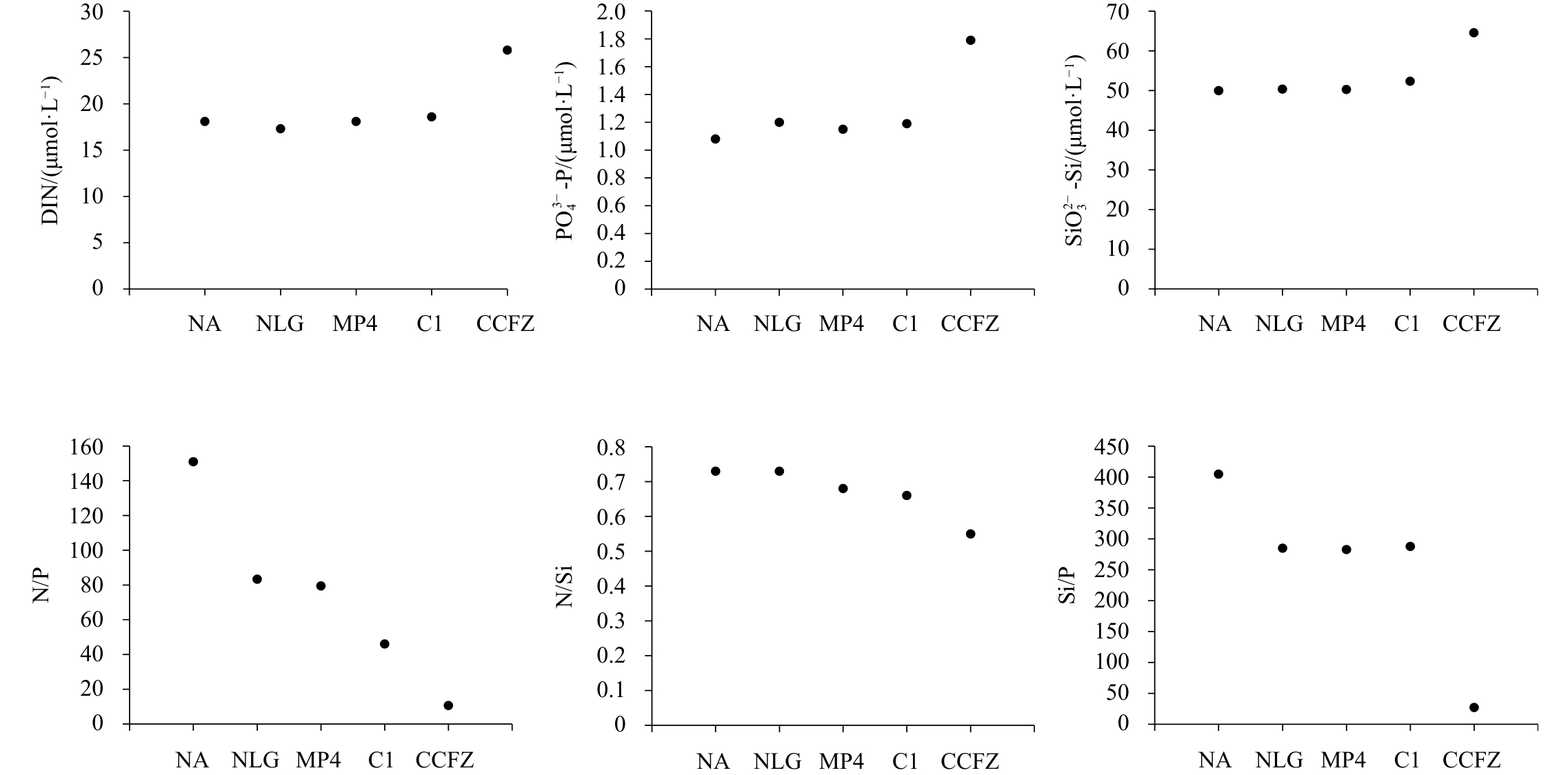
Figure 5. Average of nutrient concentrations and molar ratios in SWPO and CCFZ in 2017.

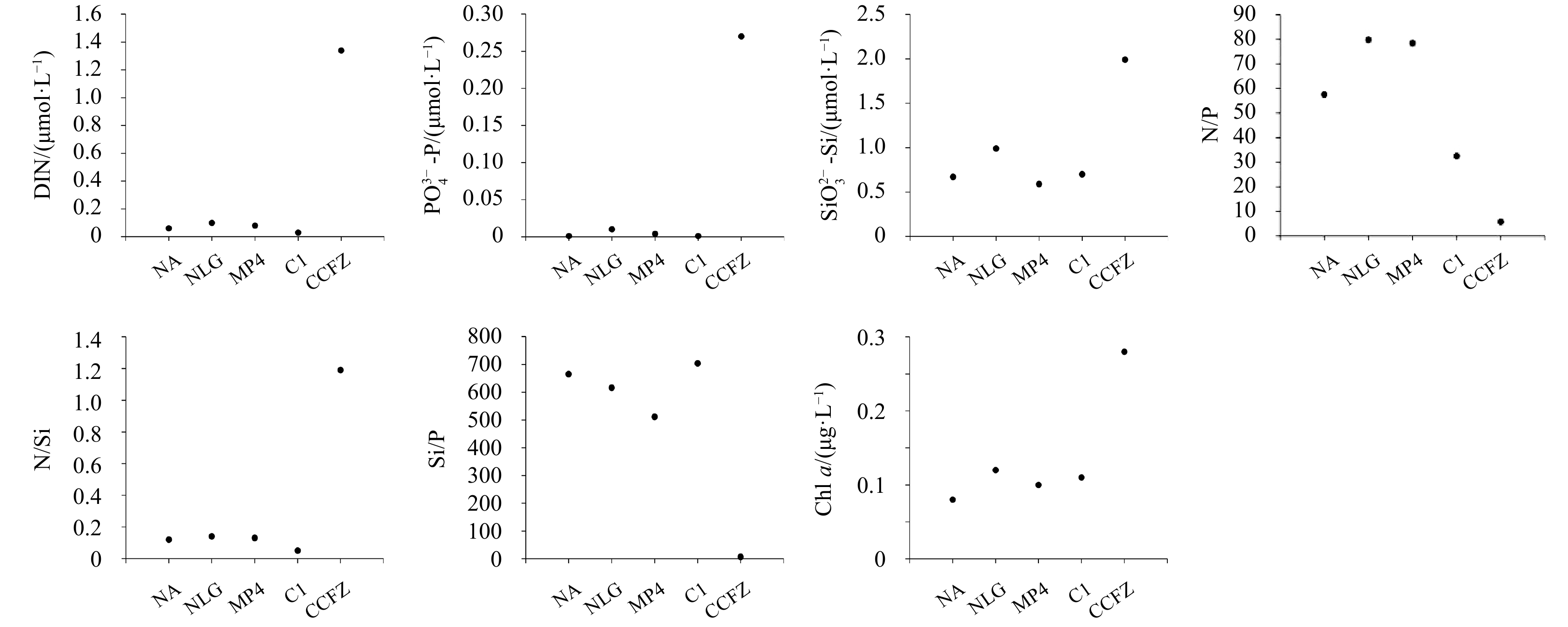
Figure 6. Average of nutrient and Chl a concentrations in 0−100 m depth layer of SWPO and CCFZ in 2017

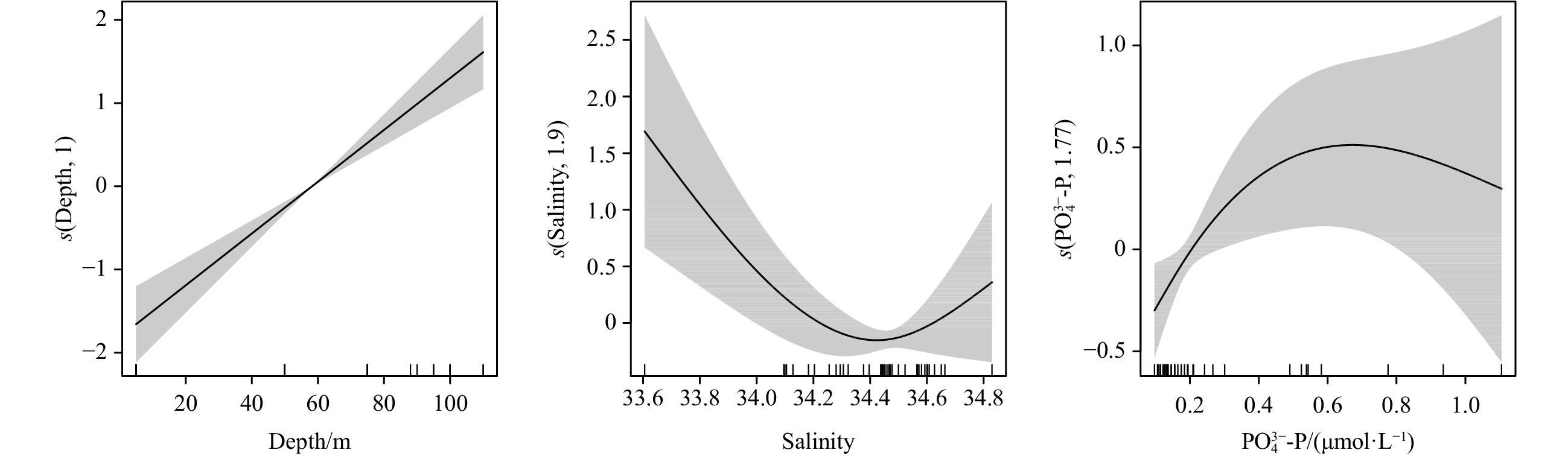
Figure 7. Generalized Additive Models (GAMs) plots illustrate significant relationship (p<0.05) between the lgChl a and depth, salinity and
${\rm{PO}}_4^{3 - }{\text -}{\rm{P}} $ . The solid line is the fitted line, while the shaded areas represent 95% confidential intervals. The numbers in the labels of y-axis denote the effective degrees of freedom; the definition of the labels of y-axis refers to Table 8.Table 1. Location and water depth of sampling stations in 2017
Station Latitude Longitude Date Depth/m CC-S06 12°58.115 1' N 153°14.585 2' W Agu. 21 5 447 CC-S01 8°30.025 6' N 154°15.151 1' W Agu. 25 5 187 KW1-S37 9°30.103 0' N 154°14.884 1' W Spet. 4−5 5 133 KW1-S05 10°04.973 9' N 154°20.038 5' W Sept. 9−10 5 173 KW1-S01 11°00.011 8' N 154°15.006 0' W Sept. 17 5 240 KW1-S40 10°11.506 6' N 154°35.663 3' W Sept. 19 5 148 CC-S09 12°59.669 3' N 154°15.523 0' W Oct. 7 5 414 CC-S10 11°59.999 0' N 154°15.006 2' W Oct. 8 5 008  下载: 导出CSV
Table 2. Technical parameters of turbidity and Chl a by CTD (SeaBird, SBE 911plus CTD)
Parameters Wave length Sensitibity Resolution Range Turbidity 700 nm 0.01 NTU 0.007 NTU 0−25 NTU Chl a 470/695 nm 0.025 μg/L 0.013 μg/L 0−50 μg/L
下载: 导出CSV
Table 3. Accuracy and precision of nutrient concentrations, DO and pH (General Administration of Quality Supervision, Inspection and Quarantine of the People’s Republic of China, Standardization Administration, 2008)
Parameters pH ${\rm{NO} }_3^ -\text{-} {\rm{N} }$
/(μmol·L−1)${\rm{NO}}_2^ -{\text -} {\rm{N}} $
/(μmol·L−1)${\rm{NH}}_4^+ {\text - }{\rm {N}} $
/(μmol·L−1)${\rm{SiO}}_3^{2 - } {\text -} {\rm{Si}}$
/(μmol·L−1)${\rm{PO}}_4^{3 - }{\text -}{\rm{P}} $
/(μmol·L−1)DO
/(μmol·L−1)Range − 0.05−16.0 0.02−4.00 0.03−8.00 0.10−25.0 0.02−4.80 5.3−1.0×10³ Accuracy ±0.02 C=2.0,
RE=±7.0%;
C=10.0,
RE=±4.0%.C= 0.5,
RE=±5.0%;
C=1.00,
RE=±3.0%.C=1.0,
RE=±7.0%;
C=7.0,
RE=±4.0%.C=4.5,
RE=±5.0%.
−
−C=0.20,
RE=±10%;
C=2.0,
RE=±3.5%.−
−
−
−Precision ±0.01 C=5.0,
RSD=±4.0%;
C=10.0,
RSD=±3.0%.C=0.3,
RSD=±5.0%;
C=1.00,
RSD=±2.0%.C=1.00,
RSD=±7.0%;
C=7.00,
RSD=±3.0%.C=4.5,
RSD=±4.0%.
−
−C=0.20,
RSD=±10%;
C=2.0,
RSD=±3.0%.C<160,
SD=±2.8;
C≥550,
SD=±4.0.Note: − repersents no data; C represents concentration; RSD, relative standard deviation; SD, standard deviation; RE, relative error.
下载: 导出CSV
Table 4. Comparing nutrient concentrations and molar ratios in water columns in SWPO and CCFZ in 2017
Area DIN/(μmol·L−1) ${\rm{PO}}_4^{3 - }{\text -}{\rm{ P}} $/(μmol·L−1) ${\rm{SiO}}_3^{2 - } {\text -} {\rm{Si}} $/(μmol·L−1) N/P N/Si Si/P NA range nd−56.8 nd−2.91 0.29−208 1.21−2284 0.00−2.90 11.6−1372 average 18.1±20.8 1.08±1.27 50.0±63.5 151±392 0.73±0.73 405±419 NLG range nd−46.1 nd−2.93 0.36−145 0.94−1157 0.01−2.90 10.8−1784 average 17.3±18.6 1.20±1.27 50.4±59.5 83.4±182 0.73±0.76 285±433 MP4 range nd−46.3 nd−2.91 0.31−153 0.50−956 nd−3.00 8.57−1166 average 18.1±20.1 1.15±1.27 50.3±61.6 79.5±162 0.68±0.71 283±353 C1 range 0.02−42.8 nd−2.75 0.50−140 13.6−106 0.04−1.75 21.9−1114 average 18.6±19.5 1.19±1.25 52.4±60.4 46.1±25.3 0.66±0.57 288±385 CCFZ range nd−61.5 0.10−3.34 0.14−174 0.01−21.7 0.00−3.09 1.05−80.0 average 25.8±19.3 1.79±1.17 64.6±63.0 10.7±6.64 0.55±0.50 27.3±23.2 Note: nd represents under detection limit.
下载: 导出CSV
Table 5. Comparing nutrient concentrations, nutrient molar ratios, and Chl a concentration in 0−100 m depth layer of SWPO and CCFZ in 2017
Area DIN/(μmol·L−1) ${\rm{PO}}_4^{3 - }{\text -}{\rm{ P}} $/(μmol·L−1) ${\rm{SiO}}_3^{2 - } {\text -} {\rm{Si}} $/(μmol·L−1) N/P N/Si Si/P Chl a/(μg·L−1) NA range nd−0.44 nd 0.29−1.01 0.54−442 0.00−0.89 286−1007 nd−0.17 average 0.06±0.11 nd±0.00 0.67±0.21 57.6±108 0.12±0.24 666±208 0.08±0.05 NLG range 0.01−0.52 nd−0.10 0.36−1.61 0.43−523 0.01−1.47 11.7−1611 nd−0.39 average 0.10±0.13 0.01±0.02 0.99±0.35 79.8±132 0.14±0.30 617±456 0.12±0.10 MP4 range nd−0.43 nd−0.05 0.36−0.87 0.54−432 0.00−0.54 10.9−867 nd−0.32 average 0.08±0.12 0.00±0.01 0.59±0.17 78.4±127 0.13±0.16 512±244 0.10±0.09 C1 range 0.02−0.05 nd 0.50−1.01 19.5−48.0 0.02−0.10 495−1007 0.05−0.19 average 0.03±0.01 nd±0.00 0.70±0.22 32.6±13.1 0.05±0.03 704±219 0.11±0.06 CCFZ range 0.00−12.4 0.10−1.11 0.14−8.73 0.00−29.3 0.00−9.10 1.05−40.4 0.01−1.02 average 1.34±2.75 0.27±0.24 1.99±2.16 5.79±7.61 1.19±2.22 7.36±6.98 0.28±0.30 Note: nd represents under detection limit.
下载: 导出CSV
Table 6. Ranges of nutrient and DO concentrations (μmol/L) in CCFZ in 1998−2017 (Tu, 2006)
Sampling time ${\rm{PO}}_4^{3 - }{\text -}{\rm{ P}} $ ${\rm{SiO}}_3^{2 - } {\text -} {\rm{Si}} $ ${\rm{NO}}_3^ - {\text -} {\rm{N}} $ ${\rm{NO}}_2^ - {\text -} {\rm{N}} $ ${\rm{NH}}_4^+ {\text - }{\rm {N}} $ DO Aug. 1998 0.07−3.09 0.00−165.9 0.00−64.12 0.00−0.85 0.00−2.04 32.8−440.2 Oct. 1999 0.00−3.28 0.00−178.3 0.00−64.35 0.01−1.58 − 28.8−438.9 Oct. 2001 0.02−3.19 0.40−152.8 0.13−54.15 0.00−0.73 0.49−1.07 22.4−442.4 Sept. 2002 0.10−3.10 0.62−133.9 0.01−50.31 − − 44.5−426.3 Sept.−Oct. 2003 0.05−3.22 2.94−152.8 0.00−52.56 0.00−0.54 − 15.0−457.5 Aug.−Oct. 2017 0.11−3.34 0.14−172.0 0.00−49.77 0.00−0.99 0.00−1.05 16.9−424.6 Note: − represents no data.
下载: 导出CSV
Table 7. Variance inflation factor (VIF) among parameters in CCFZ in 2017
Depth Temperature Salinity DO DIN ${\rm{PO}}_4^{3 - }{\text -}{\rm{ P}} $ ${\rm{SiO}}_3^{2 - } {\text -} {\rm{Si}} $ N/P N/Si Si/P Initial 6.59 10.18 2.63 9.38 31.88 35.45 64.36 14.58 4.53 13.42 Ultimate 6.51 9.32 2.61 7.54 − 8.48 − 7.84 3.68 1.16 Note: − represents no data.
下载: 导出CSV
Table 8. Statistical results of GAMs in CCFZ in 2017
Model R2 GCV n lgChl a=s(depth)+s(salinity)+s(${\rm{PO}}_4^{3 - }{\text -}{\rm{P}} $)+b 0.863 0.280 41 Note: R2 represents the adjusted proportion of total variability explained by the model; GCV, generalized cross validation score; n, the total number of samples; s, thin plate regression spline; b, a mean constant.
下载: 导出CSV
-
[1] Bahamón N, Velásquez Z, Cruzado A. 2003. Chlorophyll a and nitrogen flux in the tropical North Atlantic Ocean. Deep-Sea Research Part I: Oceanographic Research Papers, 50(10–11): 1189–1203 [2] Bange H W, Rixen T, Johansen A M, et al. 2000. A revised nitrogen budget for the Arabian Sea. Global Biogeochemical Cycles, 14(4): 1283–1297. doi: 10.1029/1999GB001228 [3] Cavender-Bares K K, Karl D M, Chisholm S W. 2001. Nutrient gradients in the western North Atlantic Ocean: Relationship to microbial community structure and comparison to patterns in the Pacific Ocean. Deep-Sea Research Part I: Oceanographic Research Papers, 48(11): 2373–2395. doi: 10.1016/S0967-0637(01)00027-9 [4] Chang B X, Devol A H, Emerson S R. 2010. Denitrification and the nitrogen gas excess in the eastern tropical South Pacific oxygen deficient zone. Deep-Sea Research Part I: Oceanographic Research Papers, 57(9): 1092–1101. doi: 10.1016/j.dsr.2010.05.009 [5] Chen Baohong, Ji Weidong, Zhou Kaiwen, et al. 2014. Nutrient and eutrophication characteristics of the Dongshan Bay, South China. Chinese Journal of Oceanology and Limnology, 32(4): 886–898. doi: 10.1007/s00343-014-3214-3 [6] Chen Bingzhang, Liu Hongbin, Huang Bangqin. 2012. Environmental controlling mechanisms on bacterial abundance in the South China Sea inferred from generalized additive models (GAMs). Journal of Sea Research, 72: 69–76. doi: 10.1016/j.seares.2012.05.012 [7] Codispoti L A, Brandes J A, Christensen J P, et al. 2001. The oceanic fixed nitrogen and nitrous oxide budgets: moving targets as we enter the anthropocene?. Scientia Marina, 65(S2): 85–105. [8] Codispoti L A, Christensen J P. 1985. Nitrification, denitrification and nitrous oxide cycling in the eastern tropical South Pacific Ocean. Marine Chemistry, 16(4): 277–300. doi: 10.1016/0304-4203(85)90051-9 [9] Deng Jianming, Qin Boqiang, Wang Bowen. 2015. Quick implementing of generalized additive models using R and its application in blue-green algal bloom forecasting. Chinese Journal of Ecology, 34(3): 835–842 [10] Feely R A, Gammon R H, Taft B A, et al. 1987. Distribution of chemical tracers in the eastern equatorial Pacific during and after the 1982–1983 El Niño/Southern Oscillation event. Journal of Geophysical Research: Oceans, 92(C6): 6545–6558. doi: 10.1029/JC092iC06p06545 [11] Fiedler P C, Lavin M F. 2006. Introduction: a review of eastern tropical Pacific oceanography. Progress in Oceanography, 69(2–4): 94–100 [12] Fiedler P C, Talley L D. 2006. Hydrography of the eastern tropical Pacific: a review. Progress in Oceanography, 69(2–4): 143–180 [13] General Administration of Quality Supervision, Inspection and Quarantine of the People’s Republic of China, Standardization Administration. 2008. GB/T 12763.4-2007 Specifications for oceanographic survey—Part 4: Survey of Chemical Parameters in Sea Water. Beijing: Standards Press of China (in Chinese) [14] Glover A G, Smith C R, Paterson G L J, et al. 2002. Polychaete species diversity in the central Pacific abyss: local and regional patterns, and relationships with productivity. Marine Ecology Progress Series, 240: 157–170. doi: 10.3354/meps240157 [15] Hastie T J, Tibshirani R J. 1990. Generalized Additive Models. New York, USA: Chapman & Hall/CRC [16] Jia Bin, Wang Tong, Wang Linna, et al. 2005. Concurvity in generalized additive models in study of air pollution. Journal of the Fourth Military Medical University, 26(3): 280–283 [17] Jones D O B, Kaiser S, Sweetman A K, et al. 2017. Biological responses to disturbance from simulated deep-sea polymetallic nodule mining. PLoS ONE, 12(2): e0171750. doi: 10.1371/journal.pone.0171750 [18] Kalvelage T, Lavik G, Jensen M M, et al. 2015. Aerobic microbial respiration in oceanic oxygen minimum zones. PLoS ONE, 10(7): e0133526. doi: 10.1371/journal.pone.0133526 [19] Kamykowski D, Zentara S J. 1990. Hypoxia in the world ocean as recorded in the historical data set. Deep-Sea Research Part A: Oceanographic Research Papers, 37(12): 1861–1874 [20] Karl D M, Björkman K M, Dore J E, et al. 2001. Ecological nitrogen-to-phosphorus stoichiometry at Station ALOHA. Deep-Sea Research Part II: Topical Studies in Oceanography, 48(8–9): 1529–1566 [21] Kessler W S. 2006. The circulation of the eastern tropical Pacific: a review. Progress in Oceanography, 69(2–4): 181–217 [22] Kim J H, Lee H, Kang J H. 2019. Associating the spatial properties of a watershed with downstream Chl a concentration using spatial analysis and generalized additive models. Water Research, 154: 387–401. doi: 10.1016/j.watres.2019.02.010 [23] Libby P S, Wheeler P A. 1997. Particulate and dissolved organic nitrogen in the central and eastern equatorial Pacific. Deep-Sea Research Part I: Oceanographic Research Papers, 44(2): 345–361. doi: 10.1016/S0967-0637(96)00089-1 [24] Loubere P. 2001. Nutrient and oceanographic changes in the eastern equatorial Pacific from the last full Glacial to the Present. Global and Planetary Change, 29(1–2): 77–98 [25] Menendez A, James R H, Lichtschlag A, et al. 2019. Controls on the chemical composition of ferromanganese nodules in the Clarion-Clipperton Fracture Zone, eastern equatorial Pacific. Marine Geology, 409: 1–14. doi: 10.1016/j.margeo.2018.12.004 [26] Ni Jianyu, Liu Xiaoqi, Zhao Hongqiao, et al. 2011. Nutrients distribution in the middle-to-low latitude zone of North Pacific. Marine Geology & Quaternary Geology, 31(2): 11–19 [27] Qiao Yinhuan, Feng Jianfeng, Cui Shangfa, et al. 2017. Long-term changes in nutrients, chlorophyll a and their relationships in a semi-enclosed eutrophic ecosystem, Bohai Bay, China. Marine Pollution Bulletin, 117(1–2): 222–228 [28] Raimbault P, Slawyk G, Boudjellal B, et al. 1999. Carbon and nitrogen uptake and export in the equatorial Pacific at 150°W: evidence of an efficient regenerated production cycle. Journal of Geophysical Research: Oceans, 104(C2): 3341–3356. doi: 10.1029/1998JC900004 [29] Raitsos D E, Korres G, Triantafyllou G, et al. 2012. Assessing chlorophyll variability in relation to the environmental regime in Pagasitikos Gulf, Greece. Journal of Marine Systems, 94 (S1): S16–S22 [30] Smith C R, De Leo F C, Bernardino A F, et al. 2008. Abyssal food limitation, ecosystem structure and climate change. Trends in Ecology & Evolution, 23(9): 518–528 [31] Song Hongjun, Zhang Xuelei, Wang Baodong, et al. 2014. Bottom-up and top-down controls of the phytoplankton standing stock off the Changjiang Estuary. Haiyang Xuebao (in Chinese), 36(8): 91–100 [32] Toggweiler J, Carson S. 1995. What are upwelling systems contributing to the ocean’s carbon and nutrient budgets?. In: Summerhays C, ed. Upwelling in the Ocean: Modern Processes and Ancient Records. New York, USA: John Wiley, 337–360 [33] Tu Xiaoxia. 2006. The research of nutrient dynamic in the China Pioneer Area of the Northeast Pacific Ocean (in Chinese) [dissertation]. Guangzhou: Guangzhou Institute of Geochemistry, Chinese Academy of Sciences [34] Volz J B, Mogollón J M, Geibert W, et al. 2018. Natural spatial variability of depositional conditions, biogeochemical processes and element fluxes in sediments of the eastern Clarion-Clipperton Zone, Pacific Ocean. Deep-Sea Research Part I: Oceanographic Research Papers, 140: 159–172. doi: 10.1016/j.dsr.2018.08.006 [35] Wang Chunzai, Enfield D B. 2001. The tropical Western Hemisphere warm pool. Geophysical Research Letters, 28(8): 1635–1638. doi: 10.1029/2000GL011763 [36] Wood S N. 2006. Generalized Additive Models: An introduction with R. Boca Raton, FL, USA: Chapman & Hall/CRC, 7–15 [37] Wu Jingfeng, Chung Shi-wei, Liang Sawwen, et al. 2003. Dissolved inorganic phosphorus, dissolved iron, and Trichodesmium in the oligotrophic South China Sea. Global Biogeochemical Cycles, 17(1): 1008 [38] Wu Yuehong, Liao Li, Wang Chunsheng, et al. 2013. A comparison of microbial communities in deep-sea polymetallic nodules and the surrounding sediments in the Pacific Ocean. Deep-Sea Research Part I: Oceanographic Research Papers, 79: 40–49. doi: 10.1016/j.dsr.2013.05.004 [39] Zhang Hanxiao, Huo Shouliang, Yeager K M, et al. 2019. Phytoplankton response to climate changes and anthropogenic activities recorded by sedimentary pigments in a shallow eutrophied lake. Science of the Total Environment, 647: 1398–1409. doi: 10.1016/j.scitotenv.2018.08.081 [40] Zhou Huimin, Feng Jianfeng, Zhu Lin. 2014. Effects of environmental factors on the chlorophyll a in central Bohai Sea with GAM. Marine Environmental Science, 33(4): 531–536 -


 点击查看大图

计量
- 文章访问数: 219
- HTML全文浏览量: 94
- PDF下载量: 7
- 被引次数: 0

