

Figure
1.
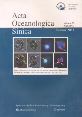
Topography of the study area and mooring location (red star). Numerals on isobaths are in m.
| Citation: | GAO Qian, XU Zhaoli. Effect of regional warming on the abundance of Pseudeuphausia sinica Wang et Chen (Euphausiacea) off the Changjiang River (Yangtze River) Estuary[J]. Acta Oceanologica Sinica, 2011, (6): 122-128. doi: 10.1007/s13131-011-0169-5

|
Previous investigations have shown that the internal solitary waves (ISWs), with large amplitudes and strong current velocities, are broadly distributed in the stratified coastal ocean and marginal seas (Jackson, 2007; Zhao et al., 2006; Stanton and Ostrovsk, 1998; Apel et al., 1985; Osborne and Burch, 1980). The South China Sea (SCS), in particular the northern SCS, is one of ocean areas where the energetic ISWs occur frequently (Wang et al., 2013; Zheng, 2017; Chen et al., 2018). In terms of the wave modes, the observed ISWs in the northern SCS could be categorized as two types, i.e., the first baroclinic mode (mode-1) and the second baroclinic mode (mode-2) (Yang et al., 2004; Chen et al., 2019). Mode-1 ISWs are characterized by only one extreme value of the vertical displacement of isotherms in the whole water column. Mode-2 ISWs typically show upward (downward) displacement of isotherms in the upper (lower) water column and three layers of currents from the uppermost to bottommost portions of a wave (Yang et al., 2010). In recent years, mode-2 ISWs in the northern SCS have been observed and reported (Yang et al., 2004; 2009; Ramp et al., 2012). According to mooring observations, Yang et al. (2009) found that mode-2 ISWs on the upper continental slope of the northern SCS occur occasionally in summer, and more frequently in winter, implying that their occurrence may be associated with the seasonal change of local stratification. Ramp et al. (2015) observed a profusion of mode-2 ISWs during 5–16 August 2011 by two cruises. They found that the waves cannot persist very far from the underwater ridge and likely do not contribute to the SCS transbasin wave phenomenon. Most recently, Chen et al. (2019) revealed a high occurrence frequency of mode-2 ISWs (including 21 mode-2 ISWs) on the northwestern SCS shelf slope west of Dongsha Atoll in December 2016, and reported an extreme mode-2 ISW with maximum upward and downward amplitudes of 73 m and 91 m, respectively. This implies that the mode-2 ISWs present in the SCS and are not difficult to be observed. Although the amplitudes and current velocities of mode-2 ISWs are smaller than those of the mode-1 ISWs, the strong currents induced by mode-2 ISWs occur in deeper water layers. Therefore, they may cause a severer threat to the underwater operation of offshore engineering, underwater navigation, and acoustic communication. Moreover, the vertical shear of the horizontal current associated with mode-2 ISWs can reach as large as 0.045 s–1, which is about 2 times that of the typical mode-1 ISWs (Qian et al., 2016). This may cause a stronger vertical mixing.
Nonlinearization of internal tide (IT) has been proved to be one of the main mechanisms for the generation of ISWs in the northern SCS. Zhao (2014) found the coherence of horizontal distribution of ISW packets observed from the SAR images with the energy fluxes of the northwestward mode-1 M2 ITs, which provides solid evidence for the scenarios that the ISWs in the northeastern SCS deep basin originate from M2 ITs at the western Luzon Strait, while the diurnal ITs play a secondary role by modifying the ISW generation (Buijsman et al., 2010; Helfrich and Grimshaw, 2008; Li and Farmer, 2011; Zhang et al., 2011). Most previous studies of the ITs in the northern SCS were restricted from the Luzon Strait to the Dongsha Atoll in the northeastern SCS but few on the continental shelf far away from the west of Dongsha Atoll, and focused on the mode-1 motions in this area (Duda et al., 2004; Yang et al., 2004; Xu et al., 2014). Based on 8-month moored acoustic Doppler current profiler observations on the northwestern SCS shelf slope west of the Dongsha Atoll, Xu et al. (2013) demonstrates that the diurnal IT are dominated by the first mode, whereas the semidiurnal tides show a variable multimodal structure: the mode-2 is dominant in summer and comparable to the first mode in spring and autumn, but the mode-1 predominates in winter.
For the generation mechanisms of mode-2 ISWs, previous studies have shown that they could be generated by the interaction between the mode-1 ISWs and topography (Helfrich and Melville, 1986; Vlasenko and Hutter, 2001; Guo and Chen, 2012; Liu et al., 2013; Lamb and Warn-Varnas, 2015) or the changes in the stratification induced by internal tides (ITs) and mesoscale eddies (Grisouard et al., 2011; Chen et al., 2014; Dong et al., 2016; Liang and Li, 2019). By laboratory experiments, Vlasenko and Hutter (2001) found that mode-1 ISWs can break into two types of ISWs, i.e., mode-1 and mode-2 ISWs, when they encounter an underwater sill. The simulative results by a two-dimensional numerical model show that both convex and concave mode-2 ISWs could be evolved from the shoaling mode-1 ISWs on the continental shelf (Lamb and Warn-Varnas, 2015). Synthetic aperture radar images show that eddy-induced change of the water stratification can result in favorable hydrographic conditions for internal wave generation (Dong et al., 2016). The resonance between mode-1 ITs and anticyclonic eddy excites mode-2 ITs, then the mode-2 ITs disintegrate into mode-2 ISWs (Dong et al., 2016). However, there have been few field observations for mode-2 ISWs generation. In this study, the mechanism of mode-2 ISWs generated by mode-2 ITs is identified by one year of mooring observations in the northern SCS from 2016 to 2017.
During the period from 30 June 2016 to 21 July 2017, a subsurface mooring, specially designed for observing ocean internal waves, was deployed to monitor the current velocity, the temperature and the salinity on the continental shelf slope west of Dongsha Atoll in the northern SCS. The mooring system was located at depth of 397 m as shown in Fig. 1. The current velocity was sampled via a 40-inch vitreous mounted, upward-looking 75 kHz acoustic-doppler-current-profile (ADCP) at depth of 380 m, 17 m above the bottom. It sampled 8-m bins every 3 min from 29 June 2016 to 13 June 2017 with a three-month gap from 20 November 2016 to 20 February 2017 due to battery failure. The depth of available current data measured by ADCP ranged from 43 m to 363 m. The vertical oscillations of the ADCP are very small, which can be ignored, because the installation depth of ADCP is close to the seabed. Between depths of 50 m and 380 m, a thermistor chain consisting of temperature loggers at every 10 m and conductivity-temperature-depth (CTD) instruments at every 50 m were attached to the mooring to monitor the temperature and the salinity every 3 min. The depths of the temperature loggers are obtained by interpolation of the depths measured by CTDs.
The horizontal current induced by the ITs can be calculated by
| $$ {u}_{\rm{IT}}(z,t)={u}_{\rm{t}}(z,t)-{u}_{\rm{ht}}\left(t\right), $$ | (1) |
where
In a continuous stratified fluid, the vertical structure of the vertical displacement
| $$ \frac{{{\rm{d}}}^{2}{\varPhi }_{n}}{{\rm{d}}{z}^{2}}+\frac{{N}^{2}\left(z\right)}{{c}_{n}^{2}}{\varPhi }_{n}=0 , $$ | (2) |
| $$ \varPhi \left(-H\right)=\varPhi \left(0\right)=0, $$ | (3) |
where
| $$ {\varPi }_{n}\left(z\right)\propto \frac{{\rm{d}}{\varPhi }_{n}}{{\rm{d}}z} . $$ | (4) |
The horizontal current induced by the IT can be approximately expressed as
| $$ {u}_{\rm{IT}}\left(z,t\right)=\sum _{n=1}^{4}{u}_{n}\left({{t}}\right){\varPi }_{n}\left(z\right) , $$ | (5) |
where
| $$ {u}_{n}\left(t\right)={\left({\varPi }_{n}^{\rm{T}}{\varPi }_{n}\right)}^{-1}{\varPi }_{n}^{\rm{T}}{u}_{\rm{IT}}, $$ | (6) |
where
Finally, the horizontal IT velocity of mode n can be written as
| $$ {u}_{n}\left(z,t\right)={u}_{n}\left(t\right){\varPi }_{n}\left(z\right) . $$ | (7) |
The depth-integrated horizontal kinetic energy (HKE) of mode n IT can be expressed as
| $$ {\rm{HKE}}_{n}=\frac{1}{2}{\int\nolimits_{-H}^{0} }{\rho \left(z\right)u}_{n}^{2}\left(z,t\right){\rm{d}}z . $$ | (8) |
Figure 2 shows two mode-2 ISWs observed on 29 and 30 July 2016, which are named No. 1 mode-2 ISW and No. 2 mode-2 ISW, respectively. No. 1 mode-2 ISW started at 17:48 and ended at 18:24 on 29 July 2016, and No. 2 mode-2 ISW started at 18:30 and ended at 19:21 on 30 July 2016. The peaks of the two mode-2 ISWs occurred at 18:06 and 19:00, respectively, indicating that the re-appearance period of them is 24.9 h, which is a characteristic time scale of type-b ISWs (Ramp et al., 2004; Chen et al., 2019). It is worth noting that the isotherms in the layer above the depth of 140 m start to sink, while the isotherms in the layer below start to rise at 13:00 on 29 July 2016. No. 1 mode-2 ISW occurred when the isotherms in the upper layer sunk deeper and the isotherms in the lower layer rose higher. No. 2 mode-2 ISW also occurred under similar hydrographic conditions. Because the re-appearance period of the two mode-2 ISWs is 24.9 h, which is close to the period of lunar day, implying that the occurrences of the two mode-2 ISWs may be associated with the IT which cause the isotherms to be compressed vertically.

In order to determine the IT features when the mode-2 ISWs occur, we extract the horizontal current induced by the IT using the ADCP data. As shown in Fig. 3b, the color contours represent the zonal currents induced by the IT calculated by Eq. (1). The dashed lines are the band-pass filter isotherms induced by diurnal and semidiurnal ITs. The cut frequency of the diurnal and semidiurnal ITs were set to [0.85 K1–1.15 O1] and [0.85 M2–1.15 S2], respectively. In order to determine the occurrence time of the mode-2 ISWs, the isotherms of 26°C and 18°C are shown in Fig. 3a. The red dotted lines are the starting time of the mode-2 ISWs. One can see that the mode-2 ISWs occur when the band-pass filter isotherms are significantly compressed, i.e., the upper isotherms are concave and the lower isotherms are convex. The zonal velocities induced by the IT show a three-layer structure with two turning points at depths of 80 m and 230 m at the time of mode-2 ISWs occurrence. These results reveal that the mode-2 ISWs occur when the isotherms significantly compressed caused by the mode-2 IT.

In order to find out whether the observed mode-2 IT signals come from the semidiurnal IT or diurnal IT, we make modal decomposition of the total, semidiurnal and diurnal ITs, respectively. Figures 4b–d show the depth-integrated horizontal kinetic energy (HKE) of different modes of total, diurnal and semidiurnal IT currents, respectively. As shown in Fig. 4b, at the onset time of No. 1 and No. 2 mode-2 ISWs, the depth-integrated HKE of mode-2 IT currents is the largest component in the total HKE. This indicates that mode-2 ISWs occur concurrently with mode-2 ITs. The depth-integrated HKE of diurnal and semidiurnal IT currents as shown in Figs 4c and d show that the mode-2 ISWs occurred at the time when the depth-integrated HKE of diurnal mode-2 IT currents reached their maximum values, instead of semidiurnal IT. Figures 5b–e show time series of zonal velocity profiles induced by diurnal IT modes 1–4 derived from mooring data. One can also see that the mode-2 ISWs do occur when the diurnal mode-2 IT is dominate. These results indicate that mode-2 ISWs occur concurrently with the diurnal mode-2 IT.


Previous investigation has shown that mode-2 ISWs can be well described by KdV equation (Chen et al., 2019). In a continuous stratified fluids, the KdV equation can be written as (Pelinovsky et al., 2007)
| $$ \frac{\partial {\eta }_{n}}{\partial t}+{c}_{n}\frac{\partial {\eta }_{n}}{\partial x}+{\alpha }_{n}{\eta }_{n}\frac{\partial {\eta }_{n}}{\partial x}+{\beta }_{n}\frac{{\partial }^{3}{\eta }_{n}}{\partial {x}^{3}}=0 , $$ | (9) |
where
| $$ {\alpha }_{n}=\frac{3{c}_{n}}{2}{\int\nolimits_{-H}^{0}}\frac{{{\rm{d}}}^{3}{\varPhi }_{n}}{{\rm{d}}{z}^{3}}{\rm{d}}z\Bigg/{\int\nolimits_{-H}^{0}}\frac{{{\rm{d}}}^{2}{\varPhi }_{n}}{{\rm{d}}{z}^{2}}{\rm{d}}z , $$ | (10) |
| $$ {\beta }_{n}=\frac{{c}_{n}}{2}{\int\nolimits _{-H}^{0}}{\varPhi }_{n}^{2}{\rm{d}}z\Bigg/{\int\nolimits _{-H}^{0}}\frac{{{\rm{d}}}^{2}{\varPhi }_{n}}{{\rm{d}}{z}^{2}}{\rm{d}}z , $$ | (11) |
where
Nonlinear coefficient
The Ursell number is defined as
| $$ {U}_{n}={\alpha }_{n}/{\beta }_{n} . $$ | (12) |
The larger the
The density stratification profile can be approximately described by hyperbolic tangent function according to mooring data (Wang, 2006).
| $$ \rho \left(z\right)={\rho }_{0}\;{\rm{exp}}\left\{\frac{\Delta \rho }{2{\rho }_{0}}{\rm{t}}{\rm{anh}}\left[\frac{-2\left(z+d\right)}{\text{δ} }\right]\right\} , $$ | (13) |
where
| $$ {N}^{2}\;\left(z\right)=-\frac{g}{\rho }\frac{{\rm{d}}\rho }{{\rm{d}}z}=\frac{g\Delta \rho }{\text{δ} {\rho }_{0}}{\rm{sech}}^{2}\left[\frac{2(z+d)}{\text{δ} }\right] . $$ | (14) |
The three parameters


The results show that a deeper and thinner pycnocline is a favorable condition for the generation of mode-2 ISWs. But the pycnocline intensity has little effect on the emergence of mode-2 ISWs. This is consistent with the numerical simulation results by Chen et al. (2014). During the observation period from 29 June 2016 to 21 July 2017, there were 42 mode-2 ISWs observed at the mooring station. More than 64% of them occurred in winter and only 14% of them occurred in summer. Because the pycnocline in the SCS is deeper in winter than that in summer, the occurrence frequency of mode-2 ISWs in the SCS in winter is much higher than that in summer. These results also explain why mode-2 ISWs are easily generated when the isotherms in the upper layer sunk deeper and the isotherms in the lower layer rose higher. Because, at the time, the pycnocline become deeper and thinner, favorable for the generation of mode-2 ISWs.
To further prove that the occurrence of the two mode-2 ISWs is related to the change of stratification and investigate the influence of the ITs on it, we calculate the mode-2 nonlinear, dispersion coefficients and the Ursell numbers with the varying stratification observed and associated with different kinds of ITs. The lack of stratification data near the surface is made up by the monthly data of World Ocean Atlas (WOA). As shown in Fig. 8, the black lines indicate the parameters calculated based on the observational stratification. Ignoring the anomalous value caused by the mode-1ISW occurred at around 16:30 on 30 July 2016, during the periods from 12:00 to 18:00 on 29 July and 13:00 to 18:30 on 30 July when mode-2 IT was the dominant component, the mode-2 Ursell number increases gradually till the mode-2 ISWs are generated. Combined with observational stratification and the results as shown in Fig. 7, it is shown that the observed mode-2 ISWs do occur at the stratified condition with a deeper and thinner pycnocline. The blue dashed lines indicate the parameters calculated based on the stratification associated with semidiurnal internal tide. One can see that the variation of the three parameters calculated based on semidiurnal internal tidal stratification is basically consistent with the observational results. However, there is a significant phase difference between the extreme values of the parameters calculated based on semidiurnal internal tidal stratification and that of observation. The phase differences are particularly evident in the Ursell numbers at the onset time of the two mode-2 ISWs. The blue solid lines as shown in Fig. 8 indicate the parameters calculated based on the stratification associated with the semidiurnal IT and diurnal mode-2 IT. After considering the influence of the diurnal mode-2 IT on the stratification, the phase differences of the Ursell number at the onset time of the two mode-2 ISWs do not exist. In other words, the mode-2 ISWs occurred when the Ursell numbers reach their maximum values under the influence of the diurnal mode-2 IT. What’s more, the maximum values of the Ursell number become bigger and more close to the observational results because of the influence of the diurnal mode-2 IT. These results indicate that when the diurnal mode-2 IT interacts with the semidiurnal IT and causes a deeper and thinner pycnocline, the mode-2 ISWs are easily excited. These results also explain why the re-appearance period of the two mode-2 ISWs is 24.9 h.

The generation mechanism of mode-2 ISWs is analyzed by mooring observations in the northern South China Sea (SCS) on 29 and 30 July 2016. Two mode-2 ISWs with a re-appearance period of 24.9 h, which is a typical feature of type-b ISWs, were observed. They occurred when the isotherms in the upper layer sunk deeper and the isotherms in the lower layer rose higher. Modal decomposition of IT horizontal currents shows that the vertical compression of the isotherms is mainly caused by diurnal mode-2 IT. The mode-2 ISWs occurred at the time when the depth-integrated HKE of diurnal mode-2 IT currents reached their maximum values, instead of semidiurnal IT. The analysis of the density stratification show that as the pycnocline becomes deeper and thinner, the mode-2 Ursell number increases, implying that a deeper and thinner pycnocline is favorable for the generation of mode-2 ISWs. However, as the pycnocline intensity increases, the mode-2 Ursell number is almost unchanged, implying that the generation of mode-2 ISWs is not directly related to the pycnocline intensity. By comparing the mode-2 nonlinear, dispersion coefficients and the Ursell numbers calculated by the stratification associated with different kinds of ITs with the observation results, it is shown that the variation of the three parameters calculated based on semidiurnal internal tidal stratification is basically consistent with the observational results. However, there is a significant phase difference between the extreme values of the parameters calculated based on semidiurnal internal tidal stratification and that of observation. The phase differences are particularly evident in the Ursell numbers at the onset time of the two mode-2 ISWs. Considering the influence of the diurnal mode-2 IT on the stratification, the phase differences of the Ursell number at the onset time of the two mode-2 ISWs do not exist. In other words, the mode-2 ISWs occurred when the Ursell numbers reach their maximum values under the influence of the diurnal mode-2 IT. What’s more, the maximum values of the Ursell number become bigger and more close to the observational results because of diurnal mode-2 IT. These results indicate that when the diurnal mode-2 IT interacts with the semidiurnal IT and causes a deeper and thinner pycnocline, the mode-2 ISWs are easily excited. These results also explain why the re-appearance period of the two mode-2 ISWs is 24.9 h.
| 1. | Zhixin Li, Jing Wang, Xu Chen, et al. Observation of Mode-2 Internal Solitary Waves in the Northern South China Sea Based on Optical Remote Sensing. IEEE Journal of Selected Topics in Applied Earth Observations and Remote Sensing, 2024, 17: 11550. doi:10.1109/JSTARS.2024.3414846 | |
| 2. | Yanliang Liu, Chalermrat Sangmanee, Qinglei Su, et al. Observed Extreme Freshening in the Central Andaman Sea Induced by Strong Positive Indian Ocean Dipole. Journal of Geophysical Research: Oceans, 2024, 129(1) doi:10.1029/2023JC020406 | |
| 3. | Zijian Cui, Weifang Jin, Tao Ding, et al. Observations of anomalously strong mode-2 internal solitary waves in the central Andaman sea by a mooring system. Deep Sea Research Part I: Oceanographic Research Papers, 2024, 208: 104300. doi:10.1016/j.dsr.2024.104300 | |
| 4. | Jing Wang, Meng Zhang, Xiangying Miao, et al. A New Method for In-Situ Measurement of Internal Solitary Waves Based on the Stimulated Raman Scattering in Optical Fibers. Journal of Ocean University of China, 2023, 22(3): 658. doi:10.1007/s11802-023-5312-3 | |
| 5. | Zhixin Li, Meng Zhang, Keda Liang, et al. Experimental Study on Optical Imaging of Convex Mode-2 Internal Solitary Waves in Calm Water. IEEE Geoscience and Remote Sensing Letters, 2023, 20: 1. doi:10.1109/LGRS.2023.3281850 | |
| 6. | Zhixin Li, Meng Zhang, Keda Liang, et al. Optical remote sensing image characteristics of large amplitude convex mode-2 internal solitary waves: an experimental study. Acta Oceanologica Sinica, 2023, 42(6): 16. doi:10.1007/s13131-022-2145-7 | |
| 7. | Qin-Ran 沁然 Li 李, Chao 超 Sun 孙, Lei 磊 Xie 谢, et al. Reconstructions of time-evolving sound-speed fields perturbed by deformed and dispersive internal solitary waves in shallow water. Chinese Physics B, 2023, 32(12): 124701. doi:10.1088/1674-1056/acf84d | |
| 8. | Longyu Huang, Jingsong Yang, Zetai Ma, et al. High-Frequency Observations of Oceanic Internal Waves from Geostationary Orbit Satellites. Ocean-Land-Atmosphere Research, 2023, 2 doi:10.34133/olar.0024 | |
| 9. | Hao Zhang, Junmin Meng, Lina Sun, et al. Observations of Reflected Internal Solitary Waves near the Continental Shelf of the Dongsha Atoll. Journal of Marine Science and Engineering, 2022, 10(6): 763. doi:10.3390/jmse10060763 | |
| 10. | Dongling Zhang, Yufei Zhang, Xu Lu, et al. Influence of Sea Surface Fluctuation on Internal Waves’ Vertical Structures in a Two-Layer Model. Ocean Science Journal, 2022, 57(2): 197. doi:10.1007/s12601-022-00071-1 | |
| 11. | Tongmu Liu, Yonggang Cao, Botao Xie, et al. A New Solitary Waves Monitoring System Based on Buoy. 2022 IEEE Asia-Pacific Conference on Image Processing, Electronics and Computers (IPEC), doi:10.1109/IPEC54454.2022.9777331 |


Supported by:
Beijing Renhe Information Technology Co. Ltd

Liang Chen, Xuejun Xiong, Quanan Zheng, Yeli Yuan, Long Yu, Yanliang Guo, Guangbing Yang, Xia Ju, Jia Sun, Zhenli Hui. Mooring observed mode-2 internal solitary waves in the northern South China Sea[J]. Acta Oceanologica Sinica, 2020, 39(11): 44-51. doi: 10.1007/s13131-020-1667-0

 DownLoad:


 DownLoad: