Identification and census statistics of multicore eddies based on sea surface height data in global oceans

1. Introduction

The term “mesoscale eddy” applied to a rotating coherent structure of ocean currents that resembles an atmospheric storm, generally refers to ocean signals with spatial scales from tens to hundreds of kilometers and temporal scales from days to months (Robinson, 2010). Eddies can be found nearly everywhere in the world ocean (Abernathey and Marshall, 2013; Chelton et al., 2011b), and they transport water, heat, salt, and energy as they propagate in the ocean (Dong et al., 2014; Roemmich and Gilson, 2001; Thompson et al., 2014; Xu et al., 2011). Eddies also play a significant role in transferring soluble carbon, chlorophyll, nutrients, and other tracers across the ocean, and have important influences on the marine ecosystem (Adams et al., 2011; Chelton et al., 2011a; Gaube, 2013). By combining satellite altimetry and Argo profiling float data, Zhang et al. (2014) found that eddy-induced zonal mass transport was comparable in magnitude to that of the large-scale wind- and thermohaline-driven circulation.

In many previous studies, eddies have been treated as independent water bodies without consideration of eddy–eddy interaction. In fact, eddy–eddy interaction is universal within the ocean (Trieling et al., 2005; Prants et al., 2011). Some studies for eddy–eddy interaction have found plenty of multicore eddy structures within the world ocean (Li and Sun, 2015; Trieling et al., 2005; Yi et al., 2015). Generally, multicore structures, which have two or more closed eddies of the same polarity within their boundaries, represent an important transitional stage in which the component eddies might experience splitting, merging, or other energy-transferring interactions. In studying eddy–eddy interaction processes, clear identification of multicore eddy structures is necessary. Chelton et al. (2011b) used a purely geometric method that based on sea level anomaly (SLA) to identify the global eddies, and recognized that recognized that their original identification algorithm can yield eddies with more than one local extremum of SLA. Note that such multiple eddies are very common in SLA data (Li and Sun, 2015; Wang et al., 2015), this problem can occur when multiple eddies are physically close together. For these multiple eddies, Yi et al. (2015) presented a Gaussian-surface-based approach to identify and characterize the multicore structures of eddies from SLA datasets and results of detecting dual-eddy structures in the South China Sea demonstrate the effectiveness of the identification approach.

Sea level anomaly (SLA) data acquired over a 23 a period (January 1993 to December 2015) were used with a threshold-free closed-contour algorithm to identify mesoscale eddies and multiple eddies within the global oceans. Multiple eddies were confirmed as multicore eddy structures through two-dimensional anisotropic Gaussian surface fitting. The rest of this paper is organized as follows. Section 2 describes the satellite data as well as the eddy detection methodology and multicore eddy’s confirmation. Section 3 provides an example of multicore eddies in the oceans and describes their evolutionary processes. Section 4 provides the census statistics of multicore eddy characteristics, including the eddy lifetimes, propagation distances, eddy propagation directions and trajectories, and kinetic properties. Finally, the summary and conclusions are given in Section 5.

2. Data and methods

2.1 Altimeter-derived SLA data

The presence and positions of mesoscale eddies were determined by analyzing SLA fields, merged and gridded multimission altimeter products, which are distributed by the Archiving Validation and Interpretation of Satellite Data in Oceanography program (AVISO). The daily SLA fields with spatial resolution of 0.25° over the global oceans spanned the 23 a period from January 1993 to December 2015. Filtering processes were used to remove residual noise and small-scale signals in the procedure of multi-altimetry data by the AVISO (Dufau et al., 2013); thus, only the large-scale and mesoscale signals were retained within the SLA fields.

2.2 Eddy identification

Generally, the mesoscale variability can be characterized as ocean signals with spatial scales of 50–500 km. So the large-scale or low-frequency SLA variabilities (e.g., the El Niño Southern Oscillation events or with the seasonal cycle of the steric expansion/contraction) were removed from the original SLA data using a high pass filter to produce a grid which includes only mesoscale variability (Chaigneau and Pizarro, 2005; Chelton et al., 2011b). A purely geometric algorithm for eddy identification based on the outermost closed contour of an SLA has been proposed by Chelton et al. (2011b). For anticyclonic eddy identification, the algorithm searches for closed SLA contour (using the simply linear interpolation based on the four adjacent grid points) beginning with an SLA threshold of –100 cm and proceeds upwards in an increment of 1 cm. A closed SLA contour which satisfies the certain conditions is considered as the eddy edge and the searching process no longer proceeds upward. For a cyclonic eddy, the searching process is similar, with the threshold beginning at +100 cm and proceeding downwards. Similar to Chelton et al. (2011b), we defined a closed SLA contour and its internal grid points as an eddy.

We increased the minimum eddy amplitude, i.e., from 1 cm in Chelton et al. (2011b) to 3 cm. The amplitude of an eddy was defined as the absolute value of the SLA difference between the eddy center and its edge. For multiple eddies that have more than one center, the amplitude was defined as the maximum SLA difference. The reason for this change was that the accuracy of measuring heights using Jason series altimeters (including Topex/Poseidon and Jason-1/2/3), which currently have optimal performance for observing ocean dynamics, is only about 2 cm in the open sea (Dufau et al., 2016). Therefore, even though the AVISO gridded SLA products represent the merging of data from different altimeters, it is difficult to claim that ocean signals under a variance of 2 cm could be captured precisely in the SLA fields, especially for the gaps in altimeter tracks that are interpolated from other observation points. This change avoids large, ameba-like eddy structures effectively because eddies with amplitude <3 cm tend to be broad and relatively flat (Chaigneau et al., 2011; Cui et al., 2016).

The choice of eddy edge in the current study constituted the greatest difference to the work of Chelton et al. (2011b). Here, the eddy edge was defined as the closed SLA contour for which the rotational speed U was greater than the translation speed c in the ocean. In the strong Western Boundary Current regions, a value of c=10 cm/s was adopted. In the open ocean, a value of c= (10−7 × latitude/50) cm/s was adopted, which varied with latitude (Fu, 2009; Fu et al., 2010). For latitudes above 50°, a constant value of c=3 cm/s was adopted (Chelton and Schlax, 1996). Here, the rotational speed U of a closed contour was considered the average of the geostrophic speed of all points in the contour, and the translation speed c referred to the change of the central position of the eddy as a function of time.

The definition of eddy scale or the eddy boundary forms an essential part of eddy identification, although such definitions are not necessarily standardized. Chelton et al. (2011b) used the outmost closed SLA contour for eddy identification, but other researchers suggested the contour with the maximum rotational speed should be used in the studies of eddies (Dong et al., 2014; Nencioli et al., 2010). The definition of eddy scale based simply on the outermost contour is not sufficiently accurate and it can often lead to enlargement of the spatial extent of an eddy. Even though the outermost water might retain a complete contour structure with the eddy interior, the water might not be trapped by the eddy and thus it will not translate with eddy movement (Flierl, 1981; Fu, 2009). In comparison, identification of an eddy boundary based on the contour line with maximum rotational speed retains the structural consistency of an eddy and it ensures the interior water is fully trapped. However, the maximum rotational speed of some contours is often >0.5 m/s, which is more common in some western boundary current regions (upper panel; Fig. 1), whereas the mean translation speed of eddies is often slow (max.: ~0.1 m/s); thus, eddy scale based on maximum rotational speed is obviously decreased. In fact, the eddy scale based on maximum rotational speed corresponds to eddy core area, the valid water that is trapped by eddies should be more expanse (Schlax and Chelton, 2016). Chelton et al. (2011b) also discussed the eddy scales from the two different definitions and found the speed-based eddy scale was more close to a Gaussian approximation for the eddy structures and should be considered as eddy kernel. So, new identification of eddy boundary should be considered.

Figure  1.  Eddy rotational velocities. a. Distribution of mean rotational velocities U on eddy contours with 1-cm interval in Gulf Stream region from SLA field on March 27, 2015. Arrows represent the surface geostrophic velocity components calculated from SLA, gray curves represent eddy boundaries determined by the UEC method, black lines represent eddy boundaries based on the maximum rotational speed method, and red points represent eddy cores that are the local extremum. The lines with color are the eddy contours with 1-cm internal that are normalized into perfect circles (the number of contours equals the eddy amplitude); the color means the value of mean rotational velocities U (cm/s). b. Variations of mean rotational velocity on eddy contours with distance to the core on March 27, 2015 globally. Each line represents an entire eddy structure with 1-cm contour interval. The numbers of the different type eddies are labeled in the panel.

DownLoad: Full-Size Img PowerPoint

Reviewing the fundamental definition of an eddy is helpful for us to understand and reasonably quantify the eddy scale. The oceanic mesoscale eddy refers to a rotating coherent structure of water that is trapped by the eddy and subsequently translates with eddy movement. The logical definition of eddy scale should recognize the extent of water validly trapped within the eddy. Chaigneau et al. (2011), Flierl (1981) and Yang et al. (2013) have suggested that the boundary of eddy water be determined by the ratio of rotational speed to translation speed; thus, the interior water is translated with eddy movement when this ratio is greater than1. Although Chelton et al. (2011b) used the outermost contour as the eddy boundary, a comparison of maximum rotational speed U and translation speed c of eddies, refers to advective nonlinear parameter U/c in their work, made them believe that the most essential feature of mesoscale eddies is nonlinearity (perhaps the most significant conclusion they thought). That means when this value of U/c exceeds 1, an eddy can advect trapped fluid within its interior as it translates, even the heat, salt and potential vorticity, as well as biogeochemical properties such as nutrients and phytoplankton (Chelton et al., 2011b; Samelson, 1992). Therefore, the definition of an eddy boundary as the closed contour for which the rotational speed U exceeds the translation speed c and coherent mesoscale features are preserved is considered appropriate and accurate. This way, both the oversize problem of eddy scope based on outermost contour is overcome and at the same time the problem of narrow range based on maximum rotational speed is also avoided.

For the world ocean, we arbitrarily chose one SLA map and we compared the results of eddy identification obtained using three methods based on different definitions of eddy scale: the outermost contour, contour with maximum rotational speed U, and contour where rotational speed U exceeds translation speed c (UEC method). The results illustrated in Fig. 1 clearly show that contour structures with high rotational speed have a parabolic shape, which implies the maximum rotational speed of these eddies is not at the boundary but generally located within the eddy interior (blue lines in Fig. 1b). Statistics show that of 2 796 eddies, the maximum speed is not found at the boundary of 1 549 of them (about 58%). On average, the contour with maximum speed is located within the central 0.7 of the eddy, i.e., the eddy scale identified based on the maximum rotational speed method is nearly half that determined using the UEC method. The scale difference is most noticeable for eddies in regions of strong currents, where the contour with maximum speed can be within the central half of the eddy, which means the difference between the two scales can be quadruple ( Fig. 1a).

The results based on the outermost contour method show many eddies rotate very slowly. The red lines in the lower panel of Fig. 1 represent eddies that have a maximum rotational speed U that is less than the translation speed c. These eddies represent about 10% of the 2 796 eddies identified and they are mainly scattered in low-latitude regions. Although the translation speed of these eddies might not be high (corresponding to general eddies), we cannot be confident that slowly rotating eddies could be effective in trapping fluid within their interior and translating that water through the ocean. Considering the need for stability and coherence of eddy structures, these eddies were ignored in this study because they cannot be identified by our proposed UEC method. Thus, the possibilities of eddy misidentification and classification of instantaneous turbulence as an eddy are reduced, which is very important both for confirmation of multicore eddy structures and for accurate recognition of splits/mergers of eddies in later research.

Here, the definitions of some properties for an eddy are given. Similarly with Chaigneau et al. (2008), the eddy size is represented by the eddy area A, which is delimited by the closed eddy boundary. The eddy scale/radius R corresponds to the equivalent radius of a circle that has the same area as the region within the eddy perimeter, which is $R = \sqrt {A/{{\text π}} } $.

Multiple eddies require more than one local extremum point of SLA in an eddy interior. Experience from experimentation has indicated that eddies with more than 3 extremum points are very unstable and short-lived, i.e., they exhibit distinct transformation of shape within a few days. Multiple eddies with 2–3 extremum points could correspond to multicore eddy structures formed because of eddy–eddy interaction and substantial interior-water exchange; however, they could also represent the misidentification of two single-core eddies because of their close spatial proximity and irregularity of the SLA contours associated with noise in the SLA fields. Multiple eddies required further processing to confirm them as a multicore eddy or as single-core eddies in close proximity.

2.3 Identification of multicore eddy structures

The structure of an idealized mesoscale eddy on the sea surface can be considered as a mathematic Gaussian shape, which is a valid and common method for studying eddy properties and dynamics (Chelton et al., 2011b; Maltrud and McClean, 2005; Wang et al., 2015). A Gaussian surface is adopted for fitting the multiple eddy structures and determining whether they compose a real multi-eddy structure or should be separated apart (Yi et al., 2015). In detail, for a multiple eddy structure H with 2–3 extremum points, each component eddy G_i(x,y) which corresponds to one extremum point is fitted by an anisotropic two dimensional Gaussian kernel expressed as:

where B represents the basal SLA of the multiple eddy structure which equals the SLA value at eddy boundary, x_i and y_i are the positions of the extremum point, σ_ix and σ_iy represent the eddy scale along the horizontal and vertical axis, A_i represents the eddy amplitude defined by the difference between the SLA of extremum point and the SLA of boundary, respectively. For a multiple eddy, B, A_i, σ_ix and σ_iy are estimated using the least-square method based on the eddy boundary and all of the eddy interior points. A case is shown in Fig. 2.

Figure  2.  Example of fitting a multicore eddy using an anisotropic two-dimensional Gaussian kernel in the SLA field. At the bottom, the black line represents the multicore eddy boundary, black asterisks represent the eddy centers, dots with color represent the SLA gridded points within the eddy interior (the colors reflect the value of the SLA), and lines with color represent the SLA contours with 2-cm intervals. The upper two independent Gauss surfaces G₁(x, y) and G₂(x, y) are fitted using the SLA gridded points, and the middle composite surface is the superposition of G₁(x, y) and G₂(x, y) with a basal SLA B (here B = –0.3 m). The fitting eddy scales σ’ are shown in the black circles at the top, and L is the distance between the composite eddy centers.

DownLoad: Full-Size Img PowerPoint

For ideal Gaussian eddies, a certain eddy scale σ’ can be defined as the SLA contour at which the average rotational speed raises to maximum and the relative vorticity reduces to zero (Chelton et al., 2011b; Flierl, 1981). The criterion for determining a real multicore eddy structure is that the distance between the composite eddy centers L(e₁, e₂) should be less than the sum of the Gaussian fitting scales (σ₁’+σ₂’) for each eddy pair, which can be expressed as L(e₁, e₂) <σ₁’+σ₂’ (Yi et al., 2014,2015). If a composite eddy fitted by a Gaussian function satisfies the criterion, it can be considered a real multicore eddy (Fig. 2). Otherwise the composite eddy structure should be considered as two single eddies because of the misidentification caused by the irregularity of SLA contours, and the identification procedure should proceed upward (downward) for anticyclone (cyclone) with an increment of 1 cm described in Section 2.2.

2.4 Multicore eddy tracking

There are many sophisticated algorithms for eddy automated tracking that have been widely applied to determine the trajectory of each eddy (Chaigneau et al., 2008; Henson and Thomas, 2008). These tracking procedures take the similar principle which considering the most similar eddies in sequential time series within a certain spatial scale as the same eddy trajectory. For single-core eddy tracking in our work, we applied the same procedure with Chaigneau et al. (2008).

In general, the oceanic mesoscale processes change slowly. The mesoscale eddies can exist in the world ocean for several months, even years in some mild oceans (Chelton et al., 2011b). Based on some knowledge of fluid mechanics, the multicore structure is not a stable state and will changes obviously in the following time (Overman and Zabusky, 1982). Not surprisingly, the lifetime of multicore eddies are expected to be shorter than that of single-core eddies (some experiments we did confirmed this guess, also see Section 3). But a transient multicore structure which exists in the ocean only few days cannot be considering as a certain mesoscale process. Experientially, only a multicore eddy structure which is found more than 6 d within one time window of 10 d can be considered as a real eddy structure. If we do not take the process, we may face a problem in the hybrid eddy tracking including the single-core eddies and multicore eddies. For example, for some eddy trajectories in the former and the latter several weeks the eddy structures both are single-core but in the central few days (e.g., 3d or 4 d) the structures are multicore. It is hard to say the multicore structure with few days have really formed in the ocean, instead they are more likely to correspond to the misidentification of multicore eddy. Notice that in this paper the multicore eddy tracking was proceeded before the single-core eddy tracking and the hybrid eddy tracking.

3. Multicore eddies in the oceans

Some previous studies of eddy–eddy interaction have found that multicore eddies exist universally within the global oceans (Li and Sun, 2015; Trieling et al., 2005; Yi et al., 2015). Generally, multicore structures, which have two closed eddies of the same polarity within their boundaries, represent an important transitional stage in their lives during which the component eddies might experience splitting or merging. To elucidate such events and to understand their dynamic processes visually, an example of multicore eddies in the oceans is examined in this section.

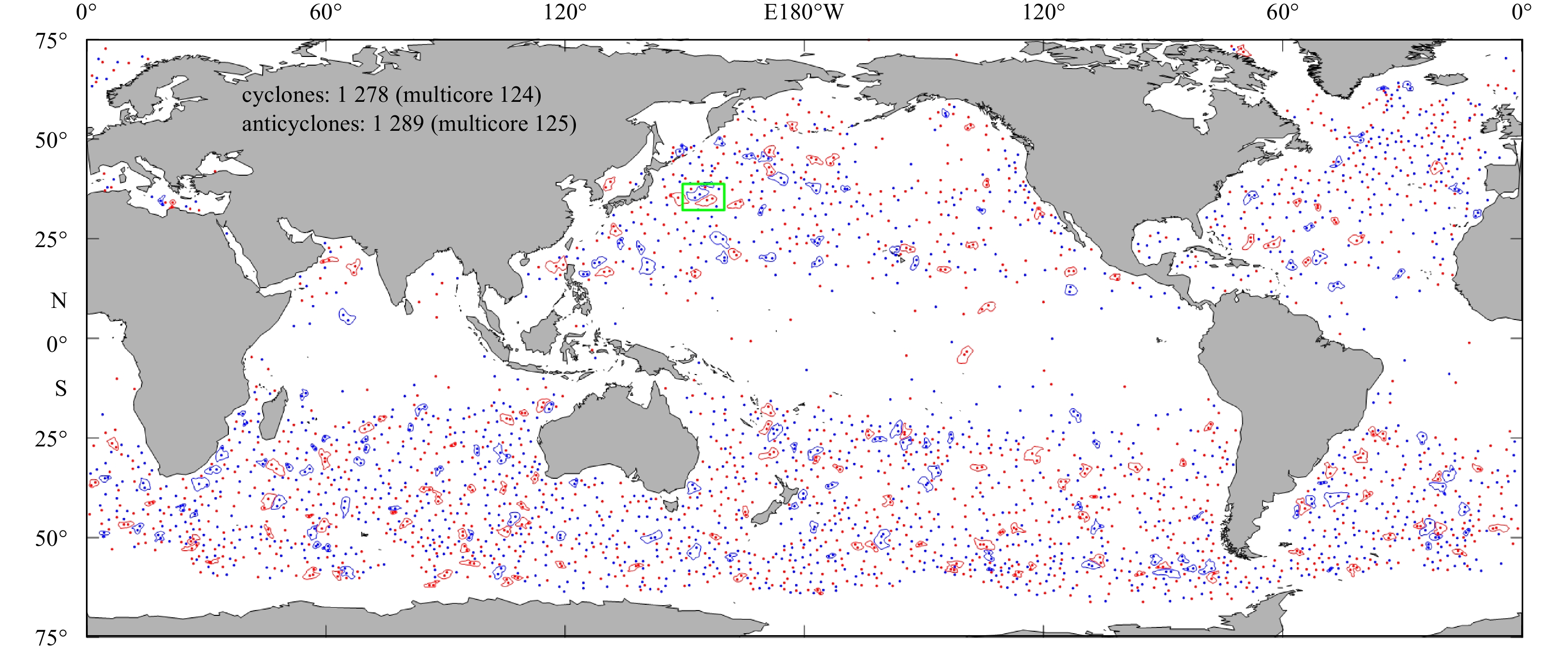
Figure 3 shows the results of eddy identification globally based on an SLA map of October 3, 2009. Application of the eddy identification procedure and the method for determination of multicore eddy structures detected about 2 300 single-core eddies and 200 multicore eddies in an arbitrary SLA field. The total number of eddies identified is slightly less than the 3 000 reported in Chelton et al. (2011b). Considering the improvements in eddy identification detailed in Section 2.2, this number is considered reasonable and acceptable. From for SLA map of October 3, 2009, 1 278 cyclonic and 1 289 anticyclonic eddies are found in global oceans, of which 124 cyclonic and 125 anticyclonic eddies are multicore structures. These multicore eddies, which are distributed throughout global oceans, mostly present an elliptical shape in which the eddy cores are geographically close. To understand the processes of multicore eddies, the green block area in Fig. 3 was selected to study the evolution of multicore eddies that was shown in Fig. 4.

Figure  3.  Eddies and multicore structures detected based on SLA map of October 3, 2009. Blue and red points represent cyclonic and anticyclonic eddies, respectively; blue and red lines represent the multicore eddy boundaries. There are 124 multicore cyclones and 125 multicore anticyclones in global oceans. The green block area in the western Pacific was selected to study the evolution of multicore eddies that was shown in Fig. 4.

DownLoad: Full-Size Img PowerPoint

Figure  4.  SLA maps of eddy evolution from September 5 to October 19, 2009. Color shading represents the value of the SLA field; arrows represent the surface geostrophic velocity components calculated from the SLA; blue and red lines represent boundaries of cyclonic and anticyclonic eddies, respectively; blue and red dots represent cyclonic and anticyclonic eddy cores, respectively; and black lines represent multicore eddies. The multicore eddy structure A_m persisted for 16 d from September 20 to October 5 before merging into a single-core eddy, and the multicore eddy structure B_m persisted for 13 d during October 2–14 before splitting into two eddies.

DownLoad: Full-Size Img PowerPoint

The SLA maps of an evolution case of multicore eddies from September 5 to October 19, 2009 are given in Fig. 4. The figure shows a case of a multicore eddy structure A_m merged into a single-core one, and another case of a multicore eddy B_m split into two eddies. The merging process of the two independently anticyclonic eddies is shown in the sequential time series of the SLA maps. At the start time (September 5), two independent eddies A1&A2 existed as single-core in the SLA map. The two eddies approached close enough to each other to instigate obvious eddy–eddy interaction and cause reduction of their spatial scales (September 9–17). Subsequently, the two eddies merged into a dual-core structure A_m that existed for 16 d from September 20 to October 5 because of the eastward movement of a strong anticyclone B to the west. Finally, the dual-core eddy A_m, which was smoothed by diffusion, evolved into a strong stable single-core eddy A on October 7. The muticore structure A_m clearly shows the evolution process of the two independently eddies A1&A2 merged into a single-core eddy A.

As for the multicore eddy B_m, it shows the splitting process of a single-core eddy B. A strong cyclonic eddy B existed as a single-core in the left of the SLA map on September 5. The cyclonic eddy B moves eastward and has a significant change in eddy shape during September 9–21 because of the nearby interaction between anticyclonic eddies A1 and A2. This cyclonic eddy B evolved into a multicore eddy B_m with itself eastward movement and the merging of multicore eddy A_m. Through westward extruding of the strong cyclonic eddy A, the multicore eddy B_m became deformed. The multicore eddy structure persisted for 13 d before finally splitting into two single-core eddies on October 14. The two single-core eddies had smaller scales compared with the multicore eddy before the split.

From the two cases of eddy merging and splitting, it can be seen that the multicore eddies change rapidly in the ocean, and their existence time is generally short; that is to say, they are not stable oceanic mesoscale structures. But the multicore eddies represent an important transitional stage in which the component eddies might experience splitting, merging, or other energy-transferring interactions. Therefore, the identification and statistics of multicore eddies are very helpful for us to understand the evolution process of eddies in global oceans. In addition, under the considertion of short existence time and unstable structure of multicore eddies, we only identified mulitcore eddy structures for at least 6 d within one time window of 10 d; otherwise, which are considered to be disordered ocean signatures.

4. Census statistics of multicore eddy structures

Globally, a statistical analysis of all multicore eddy trajectories identified by the automated tracking procedure without hybrid tracking over the 23-year period from January 1993 to December 2015 is present in this section. Here, 83 751 cyclonic and 83 406 anticyclonic multicore eddies with lifetimes >6 d are analyzed and their lifetimes, propagation distances, trajectories, and geographical distribution of properties are discussed.

4.1 Lifetimes, propagation distances, and trajectories of multicore eddies

The tracking results show 83 751 cyclonic and 83 406 anticyclonic multicore eddies with lifetimes >6 d, there is no signigicant difference between the number of them. On average, about 20 multicore eddies (exactly trajectories) emerge or generate in the world ocean daily (note the number is different with that of muticore eddies identified in daily SLA maps, the latter is about 200). Their global upper-tail cumulative histograms of lifetimes and propagation distances are shown in Fig. 5. It is apparent that multicore eddy counts fell sharply with the increasing of lifetimes and porpagation distances. In comparison with global eddies (AVISO, 2017; Chelton et al., 2011b), the lifetimes and propagation distances of multicore eddies tend to be much shorter. There are about 95% of multicore eddies with lifetimes < 30 d and there are only less than 100 eddies (close to the thousandth of all) for cyclones and anticyclones with lifetimes > 90 d. For the propagation distances, there are about 97% of multicore eddies with propagation distances < 200 km. Almost none eddies can propagate greater than 1 000 km in the ocean. The shorter lifetimes and propagation distances of multicore eddies are mainly attributable to the unstable configuration of the multicore structures. These multicore structures, which are more likely to interact with background fluids, are more easily affected by other eddies in the ocean. Therefore, the structures are easily deformed and they often split into two eddies or merge into a single eddy. In addtion, there is a slight preference for anticyclonic over cyclonic eddies with greater lifetimes and propagation distances. Specifically, there are a little more anticyclones than cyclones for lifetimes of 100 d and longer. In fact the eddy counts are very small, the preference of anticyclones with longer lifetimes is not significant. In contrast, the preference of anticyclones with propagation distances of 400 km and longer is more significant.

Figure  5.  Upper-tail cumulative histograms of lifetimes (a) and propagation distances (b) of cyclonic and anticyclonic multicore eddies over a 23-year period (January 1993 to December 2015). The lower thick and thin dashed lines represent purely cyclonic and anticyclonic multicore eddies, respectively, for which no single-core eddy was matched through hybrid tracking.

DownLoad: Full-Size Img PowerPoint

Census statistics of multicore eddies also present more than 97% of all eddies are dual-core structures and only less than 3% are triple-core structures. The signigicant difference between the numbers of dual and triple-core eddies shows that the former are more common and easily detected in the ocean. That is to say, the former stability is better than the latter (that means eddies with quad-core or more cores are more unstable). Further analyses show the lifetimes and propagation distances of dual-core eddies are longer than that of triple-core eddies, which are more direct evidences for triple-core’s instability and deformability.

The trajectories of cyclonic and anticyclonic multicore eddies are shown in Fig. 6. A striking feature is that as global eddies the multicore eddies can be found nearly everywhere in the world ocean. The multicore eddies tend to occur primarily within the Antarctic Circumpolar Current (ACC), some Western Boundary Currents (refer to the Gulf Stream and its extension, and in the region of confluence of the Kuroshio and Oyashio Currents and their eastward extensions, hereafter WBCs), and mid-latitude regions around 25°N/S. The global distribution of multicore eddies is roughly identical to that of global eddies (AVISO, 2017; Chelton et al., 2011b). Eddies with longer lifetimes (Figs 6c and d) tend to be distributed in mid-latitude areas because of the stable dynamic processes in these regions. There are fewer flow distortions and eddy–fluid interactions in these “calms seas,” such that the eddies and multicore eddies can exist for longer periods and propagate further distances. In contrast, less multicore eddies with long lifetimes can be found in the strong variable ACC and WBCs where with apparent flow distortions and rich eddy-fluid interactions. Though more eddies and multicore eddies can be yielded under the the strong flow variation (see Fig. 6a), they may be also more likely to deform under the variation and prefer to shorter lifetimes and propagation distances. Statistically, in these regions multicore eddies can exist 10–20 d and after that eddies prefer to split or merge, even or disappear. Consistently with Chelton et al. (2011b), except in some of the low latitude regions, the less multicore eddies can be observed in the regions centered at about 50°N, 160°W in the northeast Pacific and at about 50°S, 95°E in the Southeast Pacific where are called as “eddy deserts” in their paper.

Figure  6.  Trajectories of cyclonic (blue lines) and anticyclonic (red lines) multicore eddies (abbreviate as “meddy-trajs”) over the 23-year period (January 1993 to December 2015) for all eddies (a), eddies with net eastward displacement (b), eddies with lifetime≥15 d (c), and eddies with lifetime≥ 30 d (d). The trajectories of purely multicore eddies for all (e) and lifetime≥ 30 d (f) are also given. The numbers of multicore eddies of each polarity are labeled at the top of each panel.

DownLoad: Full-Size Img PowerPoint

Approximately 70% of all multicore eddies propagate westward and they occur throughout the World Ocean. Conversely, only 26 238 cyclonic and 25 677 anticyclonic multicore eddies have net eastward displacement, and these eddies are mainly restricted to regions of strong eastward currents such as the ACC and WBCs, where eddies are advected by these eastward background currents (Hughes et al., 1998; Fu, 2009). A notable feature of the multicore eddies with eastward displacement is that they have much smaller lifetimes and much shorter propagation distances than the westward eddies. Analysis shows less multicore eddies can propagate eastward more than 300 km. The short-lived eastward eddies are closely associated with strong current variations and complicated dynamic processes because of air-sea interaction.

Finally, the purely multicore eddy trajectories, which not matched with single-core eddies through hybrid tracking, are given in Figs 6e and f. Their lifetimes and propagation distances are also shown by the dashed lines in Fig. 5. The purely multicore eddies originate and terminate both as multicore structures, they neither split into two eddies nor merge into one eddy in their entire lifetimes. The numbers of the purely multicore eddies for cyclonic and anticyclonic are 11 611 and 11 132, respectively, all of which account for about 14% of all multicore eddies. These 22 743 multicore eddies have an average amplitude of about 5 cm, while that of other multicore eddies was about 16 cm, indicating considerable difference in eddy intensity. Therefore, these weaker eddies with an average radius of about 115 km exhibited a large-scale relatively flat pattern, and they tended to disappear directly under interaction with the background field. In fact, purely multicore eddies with shorter lifetime tend to be turbulence eddy-like signatures in the ocean. Similarly with all multicores eddies, the eddy counts fell sharply with the increasing of lifetimes and propagation distances. There is a slight preference of anticyclonic for the purely multicore eddies with lifetimes > 60 d and propagation distances longer than 300 km. A notable feature for right panel in Fig. 5 is that the numbers of the purely multicore eddies become closer to that of all multicore eddies with the increasing of the propagation distance. The proximity of eddy counts means that purely multicore eddies play increasingly important roles in the multicore eddies with longer propagation distance. In other words, the longer the multicore eddies propagate, they are more likely to disappear or terminate directly in the ocean (maybe due to the energy of these eddies dissipate out in the progress of eddy propagation that result in eddies not maintain enough energy for splitting or merging). The trajectories of purely multicore eddies (Figs 6e and f) show that the eddies also originate everywhere in the ocean. Note that, in the North Pacific, the distribution of pure eddies is more significant in low latitudes of about 6° north where corresponding to the North Equatorial Current and Tropical Divergence zone (Fig. 6e), and these eddies prefer to shorter lifetimes comparing the Fig. 6f.

4.2 Geographical distributions of multicore eddies

To observe the geographical distribution of multicore eddies, all of 83 751 cyclonic and 83 406 anticyclonic eddies are analyzed here and the maps of census statistics for eddy properties are shown in Fig. 7. The numbers of eddy centroids that propagate across each 1°×1° region of the World Ocean are shown in the upper panel of Fig. 7 as a frequency map of eddy occurrence. It is obvious that the ACC, WBCs and mid-latitude regions around 25°N/S have high eddy frequency (i.e., about 100–150), consistent with the distribution of trajectories of multicore eddies (Fig. 6a). Conversely, few multicore eddies are observed within the equatorial region. Chelton et al. (2011b) suggested that at these low latitudes the spatial scales of eddies are large and the amplitudes are small that result in these eddies are difficult to identified from the irregular SLA fields. The zonally averaged numbers of multicore eddies are shown by the thick lines on the right side of the upper panel (in addition, the corresponding numbers of global eddies as we tracked in this study are shown by the thin lines). The eddy counts are about 40–45 at the latitudes of 25°–60°S and about 35 at the latitudes of 20°–55°N. Southern oceans tend to have more eddies than northern oceans because of the greater ocean expanse and the west-to-east throughflow of the ACC. The numbers of multicore eddies in northern oceans tend to fluctuate in response to the effects of continental topography. Another striking feature is that at latitudes of less than 20° and greater than 60° eddy counts drop off obviously, and at latitudes of less than 10° eddy counts are very small. The significant difference (greater than one order of magnitude) between the numbers of global eddies and multicore eddies means the dominance of single-core eddies is absolute; however, the existence of multicore eddies in the world ocean cannot be ignored.

Figure  7.  Maps of the number (upper), average amplitude (middle), and average scale/radius (lower) of multicore eddies for each 1° × 1° region of the World Ocean over the 23-year period (January 1993 to December 2015). Right-hand panels show meridional profiles of the average for multicore eddies (thick lines) and global eddies (thin lines) in 1° latitude bins (equatorial region with fewer eddies is not shown).

DownLoad: Full-Size Img PowerPoint

Maps of the amplitude and radius of the multicore eddies that propagate across each 1°×1° region of the world ocean are presented in the middle and lower panels of Fig. 7, together with meridional profiles of their zonal averages. Clearly, large-amplitude (>20 cm) eddies are mainly restricted to the reasonably confined regions of highly unstable currents, such as the Gulf Stream and its extension, the Kuroshio Extension, the Agulhas Current and the Agulhas Return Current, the Antarctic Circumpolar Current, the Brazil–Malvinas Confluence region, the East Australia Current, which are highly consistent with the results of AVISO (2017) and Chelton et al. (2011b). In contrast, the multicore eddies prefer to smaller amplitudes, generally speaking less than 10 cm, in the mild oceans. Moreover the latitudinal variation of the zonally averaged eddy amplitudes is similar with that of global eddies shown in the middle right panel of Fig. 7: the maximum in the meridional profiles of mean eddy amplitudes occurs at the latitudes of about 40°N and 40°S corresponding to the WBCs; the broader peak centered near 50°S corresponds to the ACC; and the mean eddy amplitudes are smaller generally at low and high latitudes. Note that for global eddies there are an amplitude peak near 10°N which is associated with the strong eddies to the west of Central America (Palacios and Bograd, 2005; Willett et al., 2006), and a peak near 15°S which is associated with eddies that are generated between Australia and Indonesia and propagate westward across much of the south tropical Indian Ocean(Birol and Morrow, 2001; Chelton et al., 2011b; Feng and Wijffels, 2002). But the amplitude distribution of multicore eddies at latitudes of 10°N and 15°S is not significant that means eddies prefer to be stable and less likely to splitting or merging in there. Statistically, the amplitude of about 25% (20%) of all multicore eddies is <5 (>10) cm. Multicore eddies with the largest amplitude (>30 cm) are found in regions of strong and unstable currents, e.g., the ACC and WBCs. On average, multicore eddies with small amplitude have short lifetimes, which is roughly right in the mild oceans. But the eddies with large amplitude may not have longer lifetime, the distribution of multicore eddies in ACC and WBCs is a representative example. The eddy distribution of large amplitudes and short lifetimes in the strong current regions implies that eddy–fluid and eddy–eddy interaction are evident and rich splitting and merging of eddies are expected in there.

The geographical distribution of the mean eddy scale (lower panel; Fig. 7) can be characterized as decreasing monotonically from about 200 km in near-equatorial regions to about 80 km at 60°N/S. It should be noted that eddies in regions of the WBCs with larger amplitude have a larger scale than eddies in other regions at the same latitude, which implies stronger eddies tend to have larger scale. As shown in the lower right panel of Fig. 7, the latitudinal variation of the zonally averaged eddy scales is similar with that of global eddies. The mean scales of multicore eddies are < 100 km at high latitudes and are > 150 km at low latitudes. The scales are larger than that of global eddies at the same latitudes. Generally, the difference in mean scale between multicore eddies and global eddies is about 30 km, which implies that multicore eddies are typically 30%–50% larger than single-core eddies, i.e., the eddy area is at least twice as great. In addition, the scale variation with latitude is more symmetrical than with frequency and amplitude between the Southern and Northern Hemispheres.

5. Summary and conclusions

This study provides a statistical analysis of multicore eddy structures based on 23 years’ SLA data provided by AVISO from January 1993 to December 2015 in the world ocean. The multicore structures are identified through a threshold-free closed contour algorithm of SLA which is improved by some technical details. A two-dimensional anisotropic Gaussian surface fitting is used to confirm the multicore eddy structure rather than a misidentification of multiple eddies. Then the multicore eddy trajectories are obtained firstly only considering the multicore eddies through an automated tracking algorithm which adopts the most similar principle as well as single-core eddy tracking.

Generally, multicore structures have two closed eddies of the same polarity within their boundaries. From two evolution cases of multicore eddies from September 5 to October 19, 2009, it can be seen that the multicore eddies change rapidly in the ocean, and their existence time is generally short. That is to say, the multicore eddies are not stable oceanic mesoscale structures. But the multicore eddies represent an important transitional stage in which the component eddies might experience splitting, merging, or other energy-transferring interactions. Therefore, the identification and statistics of multicore eddies are very helpful for us to understand the evolution process of eddies in global oceans.

Based on 23 years’ satellite altimetry measurements, census results revealed 83 751 cyclonic and 83 406 anticyclonic multicore eddies with lifetimes >6 d. The multicore eddy counts fell sharply with the increasing of lifetimes and propagation distances. There are about 95% of multicore eddies with lifetime < 30 d and 97% of multicore eddies with propagation distance less than 200 km. In comparison with global eddies, it was found that the lifetimes and propagation distances of multicore eddies tend to be much smaller because of their inherent structural instability. In fact it is an antinomy that one hand the multicore eddies only with few days (3 or 4 d) cannot be considered as a mesoscale or quasi-mesoscale process but another hand most of them have short lifetimes in the ocean. Considering the both sides, only a multicore eddy structure which is found more than 6 d within one time window of 10 d can be considered as a real eddy structure (trajectory). The census statistics also present more than 97% are dual-core structures and only less than 3% are triple-core structures.

The multicore eddy trajectories showed they occur nearly everywhere throughout the world ocean, similar to global eddies. However, multicore eddies still have some preferences on geographical distribution. The multicore eddies prefer to occur primarily in the Antarctic Circumpolar Current (ACC), some Western Boundary Currents (WBCs), and the middle-latitude regions around 25°N/S. Most of multicore eddies, about 70%, have a net eastward displacement; while only 30% propagate eastward and are mainly restricted to regions of strong eastward currents, like ACC and WBCs, where eddies are advected with these eastward background currents. The geographical distributions of multicore eddies show many similar properties with global eddies. It was found that large-amplitude (>20 cm) eddies are mainly restricted to reasonably confined regions of highly unstable currents. In contrast, the multicore eddies prefer to smaller amplitudes in the mild oceans. It was established that the mean scale of multicore eddies decreases almost monotonically from about 200 km in near-equatorial regions to about 80 km at 60°N/S. The scale of multicore eddies was found larger than global eddies at the same latitude, i.e., the eddy area could be at least twice as large.

Acknowledgements

The altimeter products were produced by Ssalto/Duacs and distributed by Aviso, with support from Cnes (http://www.aviso.altimetry.fr/duacs/).