Figure
1.
Locations of marine stations around the China seas.
| Citation: | Guosong Wang, Xidong Wang, Hui Wang, Min Hou, Yan Li, Wenjing Fan, Yulong Liu. Evaluation on monthly sea surface wind speed of four reanalysis data sets over the China seas after 1988[J]. Acta Oceanologica Sinica, 2020, 39(1): 83-90. doi: 10.1007/s13131-019-1525-0

|
Analysis or reanalysis datasets have been used widely for research into the mechanisms of the earth’s climate system, the study of predictability, and climate monitoring (Atlas, 1987). Reanalysis has made especially great contributions to research on synoptic and planetary scale phenomena such as storm tracks, blocking, the Madden-Julian oscillation, the El Niño/Southern Oscillation and the quasi-biennial oscillation (Atlas et al., 1993; Wolfson, 1987), and verification of reproducibility of these phenomena in forecast models. Reanalysis also provides initial conditions and reference data for hindcasts of seasonal forecast systems as well as forcing fields for ocean models and chemistry-transport models.
Ocean surface wind speeds are crucial to understand and predict the short-term and long-term processes that drive our planet’s environment. As the largest source of momentum for the ocean surface, winds affect the full range of ocean movement, from individual surface waves to complete current systems. Winds along the ocean surface regulate interaction between atmosphere and ocean via modulation of air-sea exchanges of heat, moisture, gases, and particulates. With ocean covering almost three quarters of earth’s surface, this interaction has significant influence on global and regional climate. Wind speed analysis and reanalysis data sets incorporate millions of observations into a stable data assimilation system. However, observational constraints, and therefore reanalysis reliability, can considerably vary depending on the location, time period, and variable considered. The changing mix of observations, and biases in observations and models, can introduce spurious variability and trends into reanalysis output.
Oceanic surface wind speed datasets of high quality and high spatial resolution are required to understand and predict the synoptic and mesoscale air-sea interactions which affects both the atmosphere and ocean. Accadia et al. (2007) performed a comparison of satellite and forecast winds with measurements from three buoys over the Mediterranean Sea. Alvarez et al. (2013) compared various wind products and buoy wind data on seasonal and interannual climate variability in the southern Bay of Biscay. Carvalho et al. (2012) compared observed wind data among five buoys that measure the wind along the Iberian Peninsula coast, with the objective of determining which of the three reanalysis produces (NCEP-R2, ERA-int, NCEP-CFSR) more accurate wind simulations. It is concluded that spatial resolutions, assimilated measured and correction techniques allow for a more accurate and realistic representation of the local wind climate. Li et al. (2016) tested four reanalysis datasets (NCEP,CFSR, ERA-int, JRA55) by using the COSMO model in Climate Mode (CCLM) with 7-km resolution, and it is found that the downscaled simulations tend to overestimate observed low wind speeds and underestimate observed high wind speeds. In the China seaes, Kuang et al.(2015) compared three sea surface wind products in Taiwan Strait. Wang et al(2014) evaluated the distribution features of the wind energy resources in the offshore areas of China with CFSR.
In this study, the monthly homogeneity wind speeds data from ten marine stations are used to evaluate the performance of four analysis/reanalysis datasets (CCMP, CFSR, ERA-int, and JRA55) over the China seaes. This work aim to assess the accuracy of the four products of sea surface wind speeds and provide reference for future study of climate change and sea level anomaly in the China seas.
Quality controlled and homogeneity (Stephenson et al., 2008) marine stations wind speeds data is obtained from the National Marine Data and Information Service (NMDIS), and the wind speeds has been homogenized by the penalized maximum F test (PMFT) method based on reference series (Wang et al., 2017; Li et al., 2018). The position distribution can be seen from Fig.1. To quantify the potential for inter-reanalysis differences, four major reanalysis datasets were used: CCMP, CFSR, ERA-int, and JRA55. Characteristics of the 10-m wind speeds from the four datasets are summarized in Table 1. The four data sets of sea surface wind speeds products are evaluated with marine observations over the period 1988–2015, and the grid-based wind data is interpolated to the station’s locations using nearest-neighbor interpolation.
| Name | Period of record | Time step | Resolution | Model resolution | Assimilation |
| CFSR | 1979–01 to present | Sub-daily, daily, monthly | 0.5°×05° | T382 64 levels | 3DVAR |
| ERA-int | 1979–01 to present | Sub-daily, daily, monthly | ~0.75°×0.75° | T255 60 levels | 4DVAR |
| JRA55 | 1957–12 to present | Sub-daily, Monthly | 1.25°×1.25° | T319 60 levels | 4DVAR |
| CCMP | 1987–07 to present | Sub-daily, monthly | 0.25°×0.25° | / | VAM |
| Note: Characteristics of the 10-m wind speeds from the four datasets used in this paper are in bold. | |||||
 DownLoad:
CSV
DownLoad:
CSV
The Cross-Calibrated Multi-Platform (CCMP, http://podaa/c.jpl.nasa.gov/atasetlist?search =cmp) is a gridded wind vector analysis dataset produced by using satellite and buoy wind measurements (Atlas et al., 1996; Atlas et al., 2011). The CCMP V2.0 data set combines Version-7 RSS radiometer wind speeds, QuikSCAT and ASCAT scatter meter wind vectors, moored buoy wind data, and ERA-Interim model wind fields using a Variational Analysis Method (VAM) to produce four maps daily of 0.25 degree gridded vector winds.
The National Centers for Environmental Prediction (NCEP) Climate Forecast System Reanalysis (CFSR, http://rda.ucar.edu/pub/cfsr.html) is a third generation reanalysis product (Saha et al., 2010; Trenberth et al., 2010). It is a global, high resolution, coupled atmosphere-ocean-land surface-sea ice system. NCEP upgraded their operational CFS to version 2 on March 30, 2011.
The Japanese 55-year Reanalysis (JRA55, http://jra.kishou.go.jp/JRA-55/index_en.html#jra-55) is a comprehend climate dataset covering the period from 1958, when regular radiosonde observations began on a global basis, to the present (Ebita et al., 2011; Kobayashi and Iwasaki, 2016). JRA-55 is the first comprehensive reanalysis to cover the last half-century since the European Centre for Medium-Range Weather Forecasts 45-year Reanalysis (ERA-40, Uppala et al., 2005), and is also the first to apply four-dimensional variation analysis (4D-Var) to this period.
ERA-Interim (ERA-int, http://www.ecmwf.int) is European Centre for Medium-Range Weather Forecast (ECMWF) current comprehensive atmospheric reanalysis (Berrisford et al., 2011; Dee et al., 2011; Dee et al., 2013). The ERA-int atmospheric model and reanalysis system uses cycle 31r2 of ECMWF Integrated Forecast System (IFS), which was introduced operationally in September 2006.
Several statistical measures are used to assess the quality of the four data sets of sea surface wind speeds products. The bias is defined as:
| $$Bias = \frac{\operatorname{l} }{N}\sum\limits_{i = 1}^{ N} {(X_{od }^i - X_{\rm {obs}}^i)} ,$$ |
where N denotes the total pairs of records,
The root mean square error (RMSE) is defined as follows:
| $$RMSE = \sqrt {\frac{{\displaystyle\sum\limits_{i = 1}^{ N} {{{(X_{od }^i - X_{\rm {obs}}^i)}^2}} }}{N}}, $$ |
The standard deviation error (STDE) is given by:
| $$STD{E^2} = RMS{E^2} - Bia{s^2}, $$ |
Analysis/reanalysis datasets combine inaccurate and incomplete observations with imperfect models, using methods and procedures that are technically and scientifically complex. Limitations and caveats of reanalysis data mainly result from: (1) lack of observations; (2) errors in the observations, and lack of information about those errors; (3) shortcomings in the assimilating model, and lack of information about model errors; (4) shortcomings in data assimilation methodology; (5) technical errors and mistakes; (6) computational limitations.
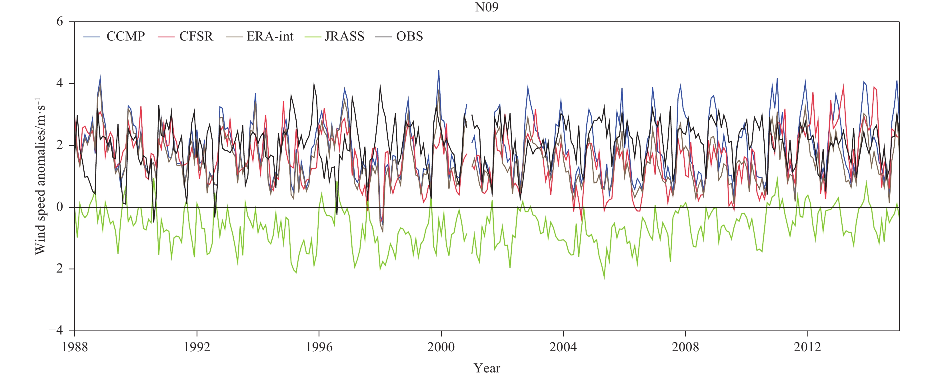
Based on the key limitations above, a comparative analysis was then carried out between four data sets of sea surface wind speeds products and observation stations. Figure 2 presents the monthly time series of wind speeds anomalies based on the four data sets of sea surface wind speeds products (CCMP, CFSR, ERA-int, JRA55) and observation stations from 1988 to 2015. It is suggested that the difference of the four data sets of sea surface wind speeds products has the smallest value at the stations C04, L03, L06, Q01 and Q05, and the wind speeds difference is between –1.5 m/s to 2 m/s. However, at the Stations D08 and K07, the wind speeds difference is quite larger, primarily because these stations are more affected by typhoon. K07 in the ERA-int generally agrees best with observations, and the wind speeds difference from CFSR ranks the worst among all products. JRA55 has the smallest difference with observations, but the negative wind speeds difference at Station N09.

To assess the detailed differences and variations, the statistics of the biases and RMSE between the observation and the four data sets at ten stations were compared. From Tables 2-3, the wind speeds bias of CCMP, CFSR, ERA-int and JRA55 are 0.910 m/s, 1.223 m/s, 0.618 m/s and 0.220 m/s, respectively. The wind speeds RMSE of CCMP, CFSR, ERA-int and JRA55 are 1.381, 1.586, 1.007 and 0.964, respectively. ERA-int and JRA55 are found to be more close to observations than CCMP and CFSR.
| Q01 | T02 | L03 | C04 | Q05 | L06 | K07 | D08 | N09 | W10 | AVE | |
| CCMP | 0.786 | 0.450 | 0.630 | 0.798 | –0.245 | –0.312 | 2.253 | 2.565 | 1.579 | 0.594 | 0.910 |
| CFSR | 0.846 | 1.073 | 0.715 | 0.964 | 0.224 | 0.301 | 2.602 | 2.803 | 1.290 | 1.410 | 1.223 |
| ERA-int | 0.434 | 0.320 | 0.625 | 0.867 | –0.159 | –0.191 | 0.970 | 1.547 | 1.188 | 0.584 | 0.618 |
| JRA55 | 0.230 | –0.192 | 0.384 | 0.418 | –0.558 | 0.147 | 2.470 | 0.527 | –0.983 | –0.241 | 0.220 |
| Note: The smallest Bias values for all of the sets of sea surface wind speeds products are in bold. | |||||||||||
DownLoad:
CSV
| Q01 | T02 | L03 | C04 | Q05 | L06 | K07 | D08 | N09 | W10 | AVE | |
| CCMP | 1.041 | 0.749 | 1.056 | 1.035 | 0.640 | 0.542 | 2.615 | 3.159 | 1.891 | 1.079 | 1.381 |
| CFSR | 1.166 | 1.486 | 0.972 | 1.255 | 0.712 | 0.539 | 3.083 | 3.277 | 1.567 | 1.801 | 1.586 |
| ERA-int | 0.656 | 0.651 | 1.050 | 1.065 | 0.508 | 0.460 | 1.185 | 1.963 | 1.424 | 1.104 | 1.007 |
| JRA55 | 0.491 | 0.512 | 0.812 | 0.661 | 0.755 | 0.555 | 2.876 | 0.893 | 1.230 | 0.860 | 0.964 |
| Note: The smallest RMSE values for all of the sets of sea surface wind speeds products are in bold. | |||||||||||
DownLoad:
CSV
It is evident that the bias and RMSE values are smaller in the Bohai Sea and the Yellow Sea for all the four data sets of sea surface wind speed products, with smallest bias of approximately 0.147 m/s and RMSE of approximately 0.460 m/s, as for Station LYG. However, the statistical errors are higher in the East China Sea and the South China Sea for all the data sets, and higher RMSE that are general larger than 1.5 m/s and can reach as high as 3.277 m/s, as for Station D08.
Taylor diagrams (Taylor, 2001) were used to summarize the relative skill of the four data sets of sea surface wind speed products. These diagrams provide a way of graphically summarizing how closely a set of patterns match observations via the metrics of the correlation, centered root mean square difference and the amplitude of their variations (represented by their standard deviations). Figure 3 reveals the Taylor diagrams for the wind speed at each observation station. The centered root-mean-square (RMS) difference between the four data sets of sea surface wind speed products and observed patterns is proportional to the distance to the point on the x-axis identified as “REF”. According to Fig. 3, the best result at the Station D08 is observed in the ERA-int, which lies closest to the REF point. The pattern correlation with observations is about 0.88.

Figure 3 suggests that the wind speeds at the Station D08 from the ERA-int and that at the W10 from the CFSR generally agree best with observations, while at the Stations Q01, K07 and N09 they agree worst with observations in the four data sets of sea surface wind speeds products. For most stations, the wind speeds from CCMP and CFSR rank the worst among all products. However, the normalized standard deviation of ERA-int and JRA55 are similar for most stations, indicating that the wind variability of ERA-int and JRA55 are quite similar to that of the observations. Note also that JRA55 has a slightly higher correlation with observations, whereas ERA-int has little larger spatial variability. In addition, the wind variability is underestimated by the four data sets of sea surface wind speeds products, with the values of the normalized standard deviation of approximately 0.70.
Prior to the launch of satellites capable of determining ocean surface wind from space, observations of ocean surface wind velocity were provided primarily by ships and buoys. While these observations are extremely useful, they also have severe limitations and are generally not adequate for global applications. For example, reports of surface wind by ships are: (1) often of poor accuracy, (2) cover only very limited regions of the world’s oceans, and (3) occur at irregular intervals in time and space. Buoys, while of higher accuracy, have extremely sparse coverage. Due to these deficiencies, analyses of surface wind that do not include space-based data can misrepresent atmospheric flow over large regions of the global oceans, and this contributes to the poor calculation of wind stress and sensible and latent heat fluxes in these regions.
Due to the sparse of conventional observational data, the four data sets of sea surface wind speeds products are assimilated a variety of satellite data, mainly from active (radar) and passive (radiometer) microwave sensors. The shortcomings of single satellite data in time span and space coverage, it is necessary to assimilate other ocean remote sensing satellites to effectively solve the problem. However, it is very easy to cause data inhomogeneity in the process of data assimilation of satellite data from different sources, and research is required to ensure data quality and the integrity of the data time series.(Azorin-Molina et al., 2014; Laapas and Venäläinen, 2017; Wan et al., 2010)
Satellite-based sensors are capable of systematically providing measurements over the entire globe. Sensors operating at microwave frequencies can make measurements of the ocean surface day and night and under nearly all-weather conditions. Both active and passive microwave sensors have been shown capable of retrieving the ocean surface wind speeds, with active microwave instruments being used to also retrieve the wind direction.
From 1988 to 1997, mainly four satellites (SSM/I F08, F10, F11 and ERS-1) provided wind observation data, and gradually stopped the data update after 1997. Four passive instruments, SMMR, SSM/I, TRMM Microwave Imager (TMI) and AMSR-E inability to extract directional ambiguities from the passive retrievals, only provided ocean surface wind speeds data.
From 1998 to 2007, SSM/I F14 and TMI satellites were launched in 1997 to provide new wind field data. Followed by the addition of QSCAT and AMSRE satellites. The second generation of satellites increased the wind direction observation function. The active sensing of the radar backscatter of centimeter-scale capillary waves allows the retrieval of ocean surface wind vectors with some directional ambiguity. Seasat, ERS (1&2), and NSCAT were designed to take advantage of this phenomenon, but the time periods for which scatterometer data is available are very limited, and not sufficient for studies of inter-annual variability and climate change.
After 2008, satellite function is more perfect, and the accuracy of data and the number of satellites also increased significantly. Meanwhile, new method was optimized for the assimilation of all available satellite surface wind data sets at high resolution.10-m winds from the ERA-40 Re-analysis were used as a background from July 1987 to December 1998 in CCMP data sets. Beginning in 1999, the benefits of 4-DVAR assimilation and increased spatial resolution make the ECMWF Operational analysis the better choice for a background of CCMP data sets.
According to the different number and types of global emission of sea surface wind field satellite since 1988, there are three obvious inhomogeneity period, namely 1988–1997, 1998–2007, 2008–2015. Based on the temperature changes, define 1988–1997 as the first period, 1998–2007 as the second period, and 2008–2015 as the third period. Statistics of the linear regress in the four data sets at ten stations over the period are compared with the observation in this paper (Barnes and Barnes, 2015; Boldina and Beninger, 2016).
Linear trends in the homogenized wind speeds series have been estimated between the four data sets of sea surface wind speeds products, and OBS wind speeds at ten stations over the period of 1988–1997 are shown in Table 4. From 1988 to 1997, the result from the observation revealed that, the trends of sea surface wind speeds showed regional differences with decreased trends from six stations. However, linear trends of sea surface wind speeds from CFSR were contrary to observations at the stations T02, C04, D08, N09 and W10, and the average RMSE was the largest of the four data sets of sea surface wind speeds products. Because the satellite wind observation technology is in the initial stage in the first period, and the data quality and coverage of the sea surface wind field are sparse, the RMSE of the four data sets of sea surface wind speeds products are larger. CCMP and ERA-int shows the same decreasing/ increasing trend which is the closest to the observation in most stations. Above all, CCMP and ERA-int are the best to agree with the OBS at ten stations over the period of 1988–1997.
| Q01 | T02 | L03 | C04 | Q05 | L06 | K07 | D08 | N09 | W10 | RMSE | |
| OBS | 0.228 | 0.842 | –0.018 | –0.229 | –0.103 | –0.376 | 0.064 | –0.593 | –0.085 | 0.246 | / |
| CCMP | 0.096 | 0.181 | –0.244 | 0.283 | –0.175 | –0.009 | 0.150 | –0.140 | –0.067 | –0.180 | 0.361 |
| CFSR | 0.224 | –0.554 | –0.140 | 0.642 | –0.164 | –0.228 | 0.531 | 0.105 | 0.300 | –0.373 | 0.631 |
| ERA–in | 0.067 | –0.038 | –0.218 | 0.306 | –0.204 | –0.147 | 0.128 | –0.146 | –0.006 | –0.308 | 0.413 |
| JRA55 | –0.022 | 0.052 | 0.039 | –0.080 | –0.281 | –0.374 | –0.435 | –0.630 | –0.535 | –0.616 | 0.440 |
| Note: Statistically significant trends are shown in boldface for p<0.10. | |||||||||||
DownLoad:
CSV
Table 5 summarizes annual wind speeds trends from 1988 to 2007. Annually, a negative trend has been found over all the stations for 1956–2013 except at T02. Meanwhile, CCMP and ERA-int show the same decreasing/ increasing trend which is the closest to the observation over all the stations except at station T02. The RMSE is significantly reduced than the period of 1988–1997, whereas the RMSE of ERA-int is the smallest (0.260).
| Q01 | T02 | L03 | C04 | Q05 | L06 | K07 | D08 | N09 | W10 | RMSE | |
| OBS | –0.115 | 0.248 | –0.165 | –0.341 | –0.096 | –0.134 | –0.028 | –0.571 | –0.483 | –0.029 | / |
| CCMP | –0.095 | 0.398 | 0.144 | –0.110 | 0.017 | 0.191 | –0.084 | –0.065 | –0.033 | 0.011 | 0.274 |
| CFSR | –0.091 | –0.349 | –0.152 | –0.114 | 0.011 | –0.241 | –0.093 | –0.091 | –0.139 | –0.082 | 0.281 |
| ERA–in | –0.165 | –0.186 | –0.063 | –0.105 | –0.048 | –0.106 | –0.123 | –0.123 | –0.070 | –0.211 | 0.260 |
| JRA55 | –0.017 | –0.278 | –0.196 | –0.167 | –0.157 | –0.239 | –0.225 | –0.110 | –0.089 | –0.237 | 0.280 |
| Note: Statistically significant trends are shown in boldface for p<0.10. | |||||||||||
DownLoad:
CSV
Finally, Table 6 shows annual wind speeds trends from 1988 to 2015. In general, there is a dominance of declining trends for all stations, the average annual wind speeds trend of China is –0.138 m/s per decade by stations, while the average trends from CCMP, CFSR, ERA-int and JRA55 were 0.050, –0.093, –0.063 and –0.080, respectively. The trend of wind speeds from CCMP is in contrast with the others and OBS. Annual wind speeds trend from ERA-int is in agreement with the declining trend detected over all stations, while linear trends of sea surface wind speeds from CCMP are contrary to observations at Stations T02, L03, Q05, L06, and W10. Compared with CCMP, CFSR, ERA-int, JRA55 and OBS, the RMSE value of CFSR and ERA-int are the smallest RMSE. It is noteworthy to highlight that, the consistency between both series constructed by different number of stations of ERA-int, which shows the same temporal variability during the period of 1988–2015.Considering the regress over the period of 1988–1997, 1998–2007 and 2008–2015 for each station, the ERA-int data set is the best result of regression over the china seas.
| Q01 | T02 | L03 | C04 | Q05 | L06 | K07 | D08 | N09 | W10 | RMSE | |
| OBS | –0.052 | –0.040 | –0.118 | –0.173 | –0.110 | –0.084 | –0.026 | –0.395 | –0.347 | –0.035 | / |
| CCMP | –0.038 | 0.280 | 0.047 | –0.040 | 0.037 | 0.169 | –0.011 | –0.025 | –0.007 | 0.086 | 0.224 |
| CFSR | –0.100 | –0.093 | –0.093 | –0.198 | –0.123 | 0.086 | –0.178 | –0.146 | –0.067 | –0.021 | 0.141 |
| ERA–in | –0.079 | –0.099 | –0.067 | –0.045 | –0.014 | –0.063 | –0.069 | –0.060 | –0.062 | –0.071 | 0.151 |
| JRA55 | 0.001 | –0.205 | –0.166 | –0.148 | –0.100 | –0.175 | –0.101 | 0.124 | 0.089 | –0.117 | 0.227 |
| Note: Statistically significant trends are shown in boldface for p<0.10. | |||||||||||
DownLoad:
CSV
In this study, a 28 year (1988–2015) monthly sea surface wind speeds of four reanalysis data sets over the China seas (CCMP, CFSR, ERA-Interim and JRA55) are evaluated.
The quality of the monthly wind speeds is first assessed by comparisons against station observations data using different statistical measures. The wind speeds bias of CCMP, CFSR, ERA-int and JRA55 are 0.91 m/s, 1.22 m/s, 0.62 m/s and 0.22 m/s, respectively. The wind speeds RMSE of CCMP, CFSR, ERA-int and JRA55 are 1.38 m/s, 1.59 m/s, 1.01 m/s and 0.96 m/s, respectively. JRA55 and ERA-int provide a realistic representation of monthly wind speeds, while CCMP and CFSR tend to overestimate observed wind speeds. The four data sets of sea surface wind speeds products all tend to underestimate observed wind speeds in the Bohai Sea and the Yellow Sea. Additionally, the corresponding trends are briefly investigated in this paper. The trend analysis of the mean wind speeds reveals that ERA-int is superior to represent homogeneity wind speeds over the China seas. Comprehensive statistical analysis suggests that ERA-Interim reanalysis is the one that will likely provide the smallest Bias and RMSE value and best agrees with the OBS in regression, which is closer to real winds for the China seas under study.
Due to the limited observation data, the conclusion of sea surface wind speeds estimation for the four data sets is only applicable to coastal waters in China. In addition, for specific weather processes (such as the typhoon process or monsoon conversion), different features are in the spatial and temporal distribution of wind field, the accuracy of which during the weather processes also remains determined. Meanwhile, wind direction is not evaluated in this paper. Future work will be conducted based on the metadata, surrounding meteorological stations as reference stations, and climate rationality analysis will be carried out on the detection of change points and correction, wind direction date from 1988 to 2015 would be homogeneity detection and correction by PMT method. The conclusions of this paper could provide reference for choosing the suitable sea surface wind field data for marine and atmospheric science research in China offshore.
| [1] |
Accadia C, Zecchetto S, Lavagnini A, et al. 2007. Comparison of 10-m wind forecasts from a regional area model and QuikSCAT scatterometer wind observations over the Mediterranean sea. Monthly Weather Review, 135(5): 1945–1960. doi: 10.1175/MWR3370.1
|
| [2] |
Alvarez I, Gomez-Gesteira M, Decastro M, et al. 2013. Comparison of different wind products and buoy wind data with seasonality and interannual climate variability in the southern Bay of Biscay (2000–2009). Deep Sea Research Part II: Topical Studies in Oceanography, 106: 38–48
|
| [3] |
Atlas D. 1987. Radar detection of hazardous small scale weather disturbances: U.S. Patent 4, 649, 388[P]. 1987–3–10
|
| [4] |
Atlas R, Hoffman R N, Ardizzone J, et al. 2011. A cross-calibrated, multiplatform ocean surface wind velocity product for meteorological and oceanographic applications. Bulletin of the American Meteorological Society, 92(2): 157–174. doi: 10.1175/2010BAMS2946.1
|
| [5] |
Atlas R, Hoffman R N, Bloom S C, et al. 1996. A multiyear global surface wind velocity dataset using SSM/I wind observations. Bulletin of the American Meteorological Society, 77(5): 869–882. doi: 10.1175/1520-0477(1996)077<0869:AMGSWV>2.0.CO;2
|
| [6] |
Atlas R, Wolfson N, Terry J. 1993. The effect of SST and soil moisture anomalies on GLA model simulations of the 1988 U. S. Summer drought. Journal of Climate, 6(11): 2034–2048
|
| [7] |
Azorin-Molina C, Vicente-Serrano S M, Mcvicar T R, et al. 2014. Homogenization and assessment of observed near-surface wind speed trends over Spain and Portugal, 1961–2011. Journal of Climate, 27(10): 3692–3712. doi: 10.1175/JCLI-D-13-00652.1
|
| [8] |
Barnes E A, Barnes R J. 2015. Estimating linear trends: simple linear regression versus epoch differences. Journal of Climate, 28(24): 9969–9976. doi: 10.1175/JCLI-D-15-0032.1
|
| [9] |
Berrisford P, Kållberg P, Kobayashi S, et al. 2011. Atmospheric conservation properties in ERA-Interim. Quarterly Journal of the Royal Meteorological Society, 137(659): 1381–1399. doi: 10.1002/qj.864
|
| [10] |
Boldina I, Beninger P G. 2016. Strengthening statistical usage in marine ecology: Linear regression. Journal of Experimental Marine Biology and Ecology, 474: 81–91. doi: 10.1016/j.jembe.2015.09.010
|
| [11] |
Carvalho D, Rocha A, Gómez-Gesteira M. 2012. Ocean surface wind simulation forced by different reanalyses: Comparison with observed data along the Iberian Peninsula coast. Ocean Modelling, 56: 31–42. doi: 10.1016/j.ocemod.2012.08.002
|
| [12] |
Dee D P, Balmaseda M, Balsamo G, et al. 2013. Toward a consistent reanalysis of the climate system. Bulletin of the American Meteorological Society, 95(8): 1235–1248
|
| [13] |
Dee D P, Uppala S M, Simmons A J, et al. 2011. The ERA-Interim reanalysis: configuration and performance of the data assimilation system. Quarterly Journal of the Royal Meteorological Society, 137(656): 553–597. doi: 10.1002/qj.828
|
| [14] |
Ebita A, Kobayashi S, Ota Y, et al. 2011. The Japanese 55-year reanalysis “JRA-55”: an interim report. SOLA, 7(1): 149–152
|
| [15] |
Kobayashi C, Iwasaki T. 2016. Brewer-Dobson circulation diagnosed from JRA-55. Journal of Geophysical Research: Atmospheres, 121(4): 1493–1510. doi: 10.1002/2015JD023476
|
| [16] |
Kuang Fangfang, Zhang Youquan, Zhang Junpeng, et al. 2015. Comparison and evaluation of three sea surface wind products in Taiwan Strait. Haiyang Xuebao (in Chinese), 37(5): 44–53
|
| [17] |
Laapas M, Venäläinen A. 2017. Homogenization and trend analysis of monthly mean and maximum wind speed time series in Finland, 1959-2015. International Journal of Climatology, 37(14): 4803–4813. doi: 10.1002/joc.5124
|
| [18] |
Li D L, Von Storch H, Geyer B. 2016. Testing reanalyses in constraining dynamical downscaling. Journal of the Meteorological Society of Japan, Ser II, 94: 47–68
|
| [19] |
Li Yan, Wang Guosong, Fan Wenjing, et al. 2018. The homogeneity study of the sea surface temperature data along the coast of the China Seas. Haiyang Xuebao (in Chinese), 40(1): 17–28
|
| [20] |
Saha S, Moorthi S, Pan H L, et al. 2010. The NCEP climate forecast system reanalysis. Bulletin of the American Meteorological Society, 91(8): 1015–1057. doi: 10.1175/2010BAMS3001.1
|
| [21] |
Stephenson T S, Goodess C M, Haylock M R, et al. 2008. Detecting inhomogeneities in Caribbean and adjacent Caribbean temperature data using sea-surface temperatures. Journal of Geophysical Research: Atmospheres, 113(D21): D21116. doi: 10.1029/2007JD009127
|
| [22] |
Taylor K E. 2001. Summarizing multiple aspects of model performance in a single diagram. Journal of Geophysical Research: Atmospheres, 106(D7): 7183–7192. doi: 10.1029/2000JD900719
|
| [23] |
Trenberth K E, Fasullo J T, Mackaro J. 2010. Atmospheric moisture transports from ocean to land and global energy flows in reanalyses. Journal of Climate, 24(18): 4907–4924
|
| [24] |
Uppala S M, Kållberg P W, Simmons A J, et al. 2005. The ERA-40 re-analysis. Quarterly Journal of the Royal Meteorological Society: A journal of the atmospheric sciences, applied meteorology and physical oceanography, 131(612): 2961–3012
|
| [25] |
Wan Hui, Wang Xiaolan, Swail V R. 2010. Homogenization and trend analysis of Canadian Near-surface wind speeds. Journal of Climate, 23(5): 1209–1225. doi: 10.1175/2009JCLI3200.1
|
| [26] |
Wang Guosong, Gao Shanhong, Wu Bingui, et al. 2014. Distribution features of wind energy resources in the offshore areas of China. Advances in Marine Science (in Chinese), 32(1): 21–29
|
| [27] |
Wang Guosong, Li Yan, Hou Min, et al. 2017. Homogeneity Study of the sea surface temperature data over the South China Seas using PMT method. Journal of Tropical Meteorology (in Chinese), 33(5): 637–643
|
| [28] |
Wolfson R. 1987. The configuration of slow-mode shocks. Journal of Geophysical Research, 92(A9): 9875–9884. doi: 10.1029/JA092iA09p09875
|
| 1. | Chongwei Zheng. A positive trend in the stability of global offshore wind energy. Acta Oceanologica Sinica, 2024, 43(1): 123. doi:10.1007/s13131-024-2345-4 | |
| 2. | Ngoc B. Trinh, Marine Herrmann, Caroline Ulses, et al. New insights into the South China Sea throughflow and water budget seasonal cycle: evaluation and analysis of a high-resolution configuration of the ocean model SYMPHONIE version 2.4. Geoscientific Model Development, 2024, 17(4): 1831. doi:10.5194/gmd-17-1831-2024 | |
| 3. | Jintao Zhou, Jin Feng, Xin Zhou, et al. Estimating Site-Specific Wind Speeds Using Gridded Data: A Comparison of Multiple Machine Learning Models. Atmosphere, 2023, 14(1): 142. doi:10.3390/atmos14010142 | |
| 4. | Liqun Jia, Shimei Wu, Bo Han, et al. Wave hindcast under tropical cyclone conditions in the South China Sea: sensitivity to wind fields. Acta Oceanologica Sinica, 2023, 42(10): 36. doi:10.1007/s13131-023-2227-1 | |
| 5. | Hanyu Deng, Gong Zhang, Changwei Liu, et al. Assessment on the Water Vapor Flux from Atmospheric Reanalysis Data in the South China Sea on 2019 Summer. Journal of Hydrometeorology, 2022, 23(6): 847. doi:10.1175/JHM-D-21-0210.1 | |
| 6. | Bikash Devkota, Kasemsan Manomaiphiboon, Piyatida Trinuruk, et al. Offshore Winds in the Gulf of Thailand: Climatology, Wind Energy Potential, Stochastic Persistence, Tropical Cyclone Influence, and Teleconnection. Asia-Pacific Journal of Atmospheric Sciences, 2022, 58(3): 315. doi:10.1007/s13143-021-00259-w | |
| 7. | Nian Liu, Zhongwei Yan, Xuan Tong, et al. Meshless Surface Wind Speed Field Reconstruction Based on Machine Learning. Advances in Atmospheric Sciences, 2022, 39(10): 1721. doi:10.1007/s00376-022-1343-8 | |
| 8. | Shimei Wu, Jingli Liu, Gong Zhang, et al. Evaluation of NCEP-CFSv2, ERA5, and CCMP wind datasets against buoy observations over Zhejiang nearshore waters. Ocean Engineering, 2022, 259: 111832. doi:10.1016/j.oceaneng.2022.111832 |


Figures(3) / Tables(6)

Supported by:
Beijing Renhe Information Technology Co. Ltd

Guosong Wang, Xidong Wang, Hui Wang, Min Hou, Yan Li, Wenjing Fan, Yulong Liu. Evaluation on monthly sea surface wind speed of four reanalysis data sets over the China seas after 1988[J]. Acta Oceanologica Sinica, 2020, 39(1): 83-90. doi: 10.1007/s13131-019-1525-0

| Name | Period of record | Time step | Resolution | Model resolution | Assimilation |
| CFSR | 1979–01 to present | Sub-daily, daily, monthly | 0.5°×05° | T382 64 levels | 3DVAR |
| ERA-int | 1979–01 to present | Sub-daily, daily, monthly | ~0.75°×0.75° | T255 60 levels | 4DVAR |
| JRA55 | 1957–12 to present | Sub-daily, Monthly | 1.25°×1.25° | T319 60 levels | 4DVAR |
| CCMP | 1987–07 to present | Sub-daily, monthly | 0.25°×0.25° | / | VAM |
| Note: Characteristics of the 10-m wind speeds from the four datasets used in this paper are in bold. | |||||
DownLoad:
CSV
| Q01 | T02 | L03 | C04 | Q05 | L06 | K07 | D08 | N09 | W10 | AVE | |
| CCMP | 0.786 | 0.450 | 0.630 | 0.798 | –0.245 | –0.312 | 2.253 | 2.565 | 1.579 | 0.594 | 0.910 |
| CFSR | 0.846 | 1.073 | 0.715 | 0.964 | 0.224 | 0.301 | 2.602 | 2.803 | 1.290 | 1.410 | 1.223 |
| ERA-int | 0.434 | 0.320 | 0.625 | 0.867 | –0.159 | –0.191 | 0.970 | 1.547 | 1.188 | 0.584 | 0.618 |
| JRA55 | 0.230 | –0.192 | 0.384 | 0.418 | –0.558 | 0.147 | 2.470 | 0.527 | –0.983 | –0.241 | 0.220 |
| Note: The smallest Bias values for all of the sets of sea surface wind speeds products are in bold. | |||||||||||
DownLoad:
CSV
| Q01 | T02 | L03 | C04 | Q05 | L06 | K07 | D08 | N09 | W10 | AVE | |
| CCMP | 1.041 | 0.749 | 1.056 | 1.035 | 0.640 | 0.542 | 2.615 | 3.159 | 1.891 | 1.079 | 1.381 |
| CFSR | 1.166 | 1.486 | 0.972 | 1.255 | 0.712 | 0.539 | 3.083 | 3.277 | 1.567 | 1.801 | 1.586 |
| ERA-int | 0.656 | 0.651 | 1.050 | 1.065 | 0.508 | 0.460 | 1.185 | 1.963 | 1.424 | 1.104 | 1.007 |
| JRA55 | 0.491 | 0.512 | 0.812 | 0.661 | 0.755 | 0.555 | 2.876 | 0.893 | 1.230 | 0.860 | 0.964 |
| Note: The smallest RMSE values for all of the sets of sea surface wind speeds products are in bold. | |||||||||||
DownLoad:
CSV
| Q01 | T02 | L03 | C04 | Q05 | L06 | K07 | D08 | N09 | W10 | RMSE | |
| OBS | 0.228 | 0.842 | –0.018 | –0.229 | –0.103 | –0.376 | 0.064 | –0.593 | –0.085 | 0.246 | / |
| CCMP | 0.096 | 0.181 | –0.244 | 0.283 | –0.175 | –0.009 | 0.150 | –0.140 | –0.067 | –0.180 | 0.361 |
| CFSR | 0.224 | –0.554 | –0.140 | 0.642 | –0.164 | –0.228 | 0.531 | 0.105 | 0.300 | –0.373 | 0.631 |
| ERA–in | 0.067 | –0.038 | –0.218 | 0.306 | –0.204 | –0.147 | 0.128 | –0.146 | –0.006 | –0.308 | 0.413 |
| JRA55 | –0.022 | 0.052 | 0.039 | –0.080 | –0.281 | –0.374 | –0.435 | –0.630 | –0.535 | –0.616 | 0.440 |
| Note: Statistically significant trends are shown in boldface for p<0.10. | |||||||||||
DownLoad:
CSV
| Q01 | T02 | L03 | C04 | Q05 | L06 | K07 | D08 | N09 | W10 | RMSE | |
| OBS | –0.115 | 0.248 | –0.165 | –0.341 | –0.096 | –0.134 | –0.028 | –0.571 | –0.483 | –0.029 | / |
| CCMP | –0.095 | 0.398 | 0.144 | –0.110 | 0.017 | 0.191 | –0.084 | –0.065 | –0.033 | 0.011 | 0.274 |
| CFSR | –0.091 | –0.349 | –0.152 | –0.114 | 0.011 | –0.241 | –0.093 | –0.091 | –0.139 | –0.082 | 0.281 |
| ERA–in | –0.165 | –0.186 | –0.063 | –0.105 | –0.048 | –0.106 | –0.123 | –0.123 | –0.070 | –0.211 | 0.260 |
| JRA55 | –0.017 | –0.278 | –0.196 | –0.167 | –0.157 | –0.239 | –0.225 | –0.110 | –0.089 | –0.237 | 0.280 |
| Note: Statistically significant trends are shown in boldface for p<0.10. | |||||||||||
DownLoad:
CSV
| Q01 | T02 | L03 | C04 | Q05 | L06 | K07 | D08 | N09 | W10 | RMSE | |
| OBS | –0.052 | –0.040 | –0.118 | –0.173 | –0.110 | –0.084 | –0.026 | –0.395 | –0.347 | –0.035 | / |
| CCMP | –0.038 | 0.280 | 0.047 | –0.040 | 0.037 | 0.169 | –0.011 | –0.025 | –0.007 | 0.086 | 0.224 |
| CFSR | –0.100 | –0.093 | –0.093 | –0.198 | –0.123 | 0.086 | –0.178 | –0.146 | –0.067 | –0.021 | 0.141 |
| ERA–in | –0.079 | –0.099 | –0.067 | –0.045 | –0.014 | –0.063 | –0.069 | –0.060 | –0.062 | –0.071 | 0.151 |
| JRA55 | 0.001 | –0.205 | –0.166 | –0.148 | –0.100 | –0.175 | –0.101 | 0.124 | 0.089 | –0.117 | 0.227 |
| Note: Statistically significant trends are shown in boldface for p<0.10. | |||||||||||
DownLoad:
CSV
| Name | Period of record | Time step | Resolution | Model resolution | Assimilation |
| CFSR | 1979–01 to present | Sub-daily, daily, monthly | 0.5°×05° | T382 64 levels | 3DVAR |
| ERA-int | 1979–01 to present | Sub-daily, daily, monthly | ~0.75°×0.75° | T255 60 levels | 4DVAR |
| JRA55 | 1957–12 to present | Sub-daily, Monthly | 1.25°×1.25° | T319 60 levels | 4DVAR |
| CCMP | 1987–07 to present | Sub-daily, monthly | 0.25°×0.25° | / | VAM |
| Note: Characteristics of the 10-m wind speeds from the four datasets used in this paper are in bold. | |||||
| Q01 | T02 | L03 | C04 | Q05 | L06 | K07 | D08 | N09 | W10 | AVE | |
| CCMP | 0.786 | 0.450 | 0.630 | 0.798 | –0.245 | –0.312 | 2.253 | 2.565 | 1.579 | 0.594 | 0.910 |
| CFSR | 0.846 | 1.073 | 0.715 | 0.964 | 0.224 | 0.301 | 2.602 | 2.803 | 1.290 | 1.410 | 1.223 |
| ERA-int | 0.434 | 0.320 | 0.625 | 0.867 | –0.159 | –0.191 | 0.970 | 1.547 | 1.188 | 0.584 | 0.618 |
| JRA55 | 0.230 | –0.192 | 0.384 | 0.418 | –0.558 | 0.147 | 2.470 | 0.527 | –0.983 | –0.241 | 0.220 |
| Note: The smallest Bias values for all of the sets of sea surface wind speeds products are in bold. | |||||||||||
| Q01 | T02 | L03 | C04 | Q05 | L06 | K07 | D08 | N09 | W10 | AVE | |
| CCMP | 1.041 | 0.749 | 1.056 | 1.035 | 0.640 | 0.542 | 2.615 | 3.159 | 1.891 | 1.079 | 1.381 |
| CFSR | 1.166 | 1.486 | 0.972 | 1.255 | 0.712 | 0.539 | 3.083 | 3.277 | 1.567 | 1.801 | 1.586 |
| ERA-int | 0.656 | 0.651 | 1.050 | 1.065 | 0.508 | 0.460 | 1.185 | 1.963 | 1.424 | 1.104 | 1.007 |
| JRA55 | 0.491 | 0.512 | 0.812 | 0.661 | 0.755 | 0.555 | 2.876 | 0.893 | 1.230 | 0.860 | 0.964 |
| Note: The smallest RMSE values for all of the sets of sea surface wind speeds products are in bold. | |||||||||||
| Q01 | T02 | L03 | C04 | Q05 | L06 | K07 | D08 | N09 | W10 | RMSE | |
| OBS | 0.228 | 0.842 | –0.018 | –0.229 | –0.103 | –0.376 | 0.064 | –0.593 | –0.085 | 0.246 | / |
| CCMP | 0.096 | 0.181 | –0.244 | 0.283 | –0.175 | –0.009 | 0.150 | –0.140 | –0.067 | –0.180 | 0.361 |
| CFSR | 0.224 | –0.554 | –0.140 | 0.642 | –0.164 | –0.228 | 0.531 | 0.105 | 0.300 | –0.373 | 0.631 |
| ERA–in | 0.067 | –0.038 | –0.218 | 0.306 | –0.204 | –0.147 | 0.128 | –0.146 | –0.006 | –0.308 | 0.413 |
| JRA55 | –0.022 | 0.052 | 0.039 | –0.080 | –0.281 | –0.374 | –0.435 | –0.630 | –0.535 | –0.616 | 0.440 |
| Note: Statistically significant trends are shown in boldface for p<0.10. | |||||||||||
| Q01 | T02 | L03 | C04 | Q05 | L06 | K07 | D08 | N09 | W10 | RMSE | |
| OBS | –0.115 | 0.248 | –0.165 | –0.341 | –0.096 | –0.134 | –0.028 | –0.571 | –0.483 | –0.029 | / |
| CCMP | –0.095 | 0.398 | 0.144 | –0.110 | 0.017 | 0.191 | –0.084 | –0.065 | –0.033 | 0.011 | 0.274 |
| CFSR | –0.091 | –0.349 | –0.152 | –0.114 | 0.011 | –0.241 | –0.093 | –0.091 | –0.139 | –0.082 | 0.281 |
| ERA–in | –0.165 | –0.186 | –0.063 | –0.105 | –0.048 | –0.106 | –0.123 | –0.123 | –0.070 | –0.211 | 0.260 |
| JRA55 | –0.017 | –0.278 | –0.196 | –0.167 | –0.157 | –0.239 | –0.225 | –0.110 | –0.089 | –0.237 | 0.280 |
| Note: Statistically significant trends are shown in boldface for p<0.10. | |||||||||||
| Q01 | T02 | L03 | C04 | Q05 | L06 | K07 | D08 | N09 | W10 | RMSE | |
| OBS | –0.052 | –0.040 | –0.118 | –0.173 | –0.110 | –0.084 | –0.026 | –0.395 | –0.347 | –0.035 | / |
| CCMP | –0.038 | 0.280 | 0.047 | –0.040 | 0.037 | 0.169 | –0.011 | –0.025 | –0.007 | 0.086 | 0.224 |
| CFSR | –0.100 | –0.093 | –0.093 | –0.198 | –0.123 | 0.086 | –0.178 | –0.146 | –0.067 | –0.021 | 0.141 |
| ERA–in | –0.079 | –0.099 | –0.067 | –0.045 | –0.014 | –0.063 | –0.069 | –0.060 | –0.062 | –0.071 | 0.151 |
| JRA55 | 0.001 | –0.205 | –0.166 | –0.148 | –0.100 | –0.175 | –0.101 | 0.124 | 0.089 | –0.117 | 0.227 |
| Note: Statistically significant trends are shown in boldface for p<0.10. | |||||||||||
 DownLoad:


 DownLoad: