Jingling Yang, Shaocai Jiang, Junshan Wu, Lingling Xie, Shuwen Zhang, Peng Bai. Effects of wave-current interaction on the waves, cold-water mass and transport of diluted water in the Beibu Gulf[J]. Acta Oceanologica Sinica, 2020, 39(1): 25-40. doi: 10.1007/s13131-019-1529-9
Citation:
Jingling Yang, Shaocai Jiang, Junshan Wu, Lingling Xie, Shuwen Zhang, Peng Bai. Effects of wave-current interaction on the waves, cold-water mass and transport of diluted water in the Beibu Gulf[J]. Acta Oceanologica Sinica, 2020, 39(1): 25-40. doi: 10.1007/s13131-019-1529-9
Jingling Yang, Shaocai Jiang, Junshan Wu, Lingling Xie, Shuwen Zhang, Peng Bai. Effects of wave-current interaction on the waves, cold-water mass and transport of diluted water in the Beibu Gulf[J]. Acta Oceanologica Sinica, 2020, 39(1): 25-40. doi: 10.1007/s13131-019-1529-9
Citation:
Jingling Yang, Shaocai Jiang, Junshan Wu, Lingling Xie, Shuwen Zhang, Peng Bai. Effects of wave-current interaction on the waves, cold-water mass and transport of diluted water in the Beibu Gulf[J]. Acta Oceanologica Sinica, 2020, 39(1): 25-40. doi: 10.1007/s13131-019-1529-9
Guangdong Province Key Laboratory for Coastal Ocean Variation and Disaster Prediction, College of Ocean and Meteorology, Guangdong Ocean University, Zhanjiang 524088, China
2.
Marine Resources Big Data Center of South China Sea, Southern Marine Science and Engineering Guangdong Laboratory (Zhanjiang), Zhanjiang 524025, China
3.
Beihai Marine Environmental Monitoring Center, South China Sea Bureau of Ministry of Natural Resources, Beihai 536000, China
4.
East China Sea Bureau of Ministry of Natural Resources, Shanghai 200137, China
5.
Institute of Marine Science, College of Science, Shantou University, Shantou 515063, China
Funds:
The Program for Scientific Research Start-up Funds of Guangdong Ocean University under contract No. 101302/R18001; the Fund of Southern Marine Science and Engineering Guangdong Laboratory (Zhanjiang) under contract No. ZJW-2019-08; the National Key Research and Development Program of China under contract No. 2016YFC1401403; the National Natural Science Foundation of China under contract Nos 41476009 and 41776034.
Wave-current interaction and its effects on the hydrodynamic environment in the Beibu Gulf (BG) have been investigated via employing the Coupled Ocean–Atmosphere–Wave–Sediment Transport (COAWST) modeling system. The model could simulate reasonable hydrodynamics in the BG when validated by various observations. Vigorous tidal currents refract the waves efficiently and make the seas off the west coast of Hainan Island be the hot spot where currents modulate the significant wave height dramatically. During summer, wave-enhanced bottom stress could weaken the near-shore component of the gulf-scale cyclonic-circulation in the BG remarkably, inducing two major corresponding adjustments: Model results reveal that the deep-layer cold water from the southern BG makes critical contribution to maintaining the cold-water mass in the northern BG Basin. However, the weakened background circulation leads to less cold water transported from the southern gulf to the northern gulf, which finally triggers a 0.2°C warming in the cold-water mass area; In the top areas of the BG, the suppressed background circulation reduces the transport of the diluted water to the central gulf. Therefore, more freshwater could be trapped locally, which then triggers lower sea surface salinity (SSS) in the near-field and higher SSS in the far-field.
Wave-current interaction has been well recognized to play an important role in modulating coastal and near-shore hydrodynamics (e.g. Longuet-Higgins and Stewart, 1962; Svendsen, 1984; Wolf and Prandle, 1999). Waves can make contributions to the circulation, which in turn modifies the waves, thus complicated wave-current feedback system would be established. On one hand, currents can exert refracting and blocking effects on the waves; currents can also modify the bottom friction felt by waves (Vincent, 1979; Ris et al., 1999). Meanwhile, the water level can also affect wave characters by changing the water depth (Pleskachevsky et al., 2009). On the other hand, waves can provide excessive momentum and mass fluxes to the currents, leading to critical adjustments of the mean flow and triggering a variety of classic phenomena, for instance, the wave setup and setdown (Longuet-Higgins and Stewart, 1962), the undertow (Svendsen, 1984), and the wave-driven along-shore currents (Longuet-Higgins, 1970).
Previous studies have emphasized the importance of various wave-current interactive mechanisms. For the cases that waves are dramatically modified, the numerical investigation of Osuna and Monbaliu (2004) revealed that differences of significant wave heights and mean wave periods could reach up to about 0.2 m and 1 s when current speed up to 1 m/s. Fan et al. (2009) reported that taking currents into consideration could improve performance of wave modeling since following currents could reduce the wave energy and then decrease the significant wave height. When waves encounter opposing currents, the significant wave heights could be increased by as much as 20% (Warner et al., 2010). In the tide-dominated estuary investigated by Bolaños et al. (2014), significant wave height and wave period were dominated by the time-varying water depth, further, Doppler shift induced by currents could exert a prime effect on the wave periods.
Conversely, currents are also adjustable to waves. Xie et al. (2001) demonstrated that waves could trigger enhanced surface and bottom shear stress, and the former one helped to accelerate the current speed in the upper layer while the later one weakened that in the bottom layer, which lead to vital adjustment of the South Atlantic Bight circulation. When wave effects are involved in, Beardsley et al. (2013) reported that higher storm surge and more inundation area would be simulated during a nor’easter event, meanwhile, the coastal current structure also changed dramatically. In the northern Adriatic Sea, the surface drifter trajectory was better reproduced when taking wave-breaking effect into account (Carniel et al., 2009). Olabarrieta et al. (2011) identified that the wave-breaking-induced acceleration served as a leading term in the horizontal momentum balance in the inlet area of the Willapa Bay. Investigation of Niu and Xia (2017) proposed vital roles played by wave-induced surface and radiation stresses in both the seasonal-mean and episodic-scale dynamics of Lake Erie.
In the china seas, significance of wave-current interaction has also been highlighted by previous studies. In the Yellow Sea, wave-mixing was recognized as a key role in the formation of the upper mixed layer in spring and summer (Qiao et al., 2004) and wave-mixing could increase the mixed layer thickness greatly (Yang et al., 2004). The surface boundary layer thickness in the Yellow Sea could be better solved when wave enhanced vertical mixing due to wave breaking was introduced (Zhang et al., 2011). Study of Zhao et al. (2017) focusing on two storms striking the South China Sea (SCS) revealed that wave-induced vertical mixing could lead to deeper thermocline and cooler surface, decreasing the typhoon intensity. When evaluated effects of wave-current interaction on storm surge in the northern SCS, Zhang et al. (2018) suggested improved simulation by both radiation-stress and vortex force formulations. Recently, Gong et al. (2018) indicated the waves could affect the dispersal of the Zhujiang River (Pearl River) plume by increasing surface wind stress and bottom drag stress, enhancing vertical mixing and supplying 3-D wave forces.
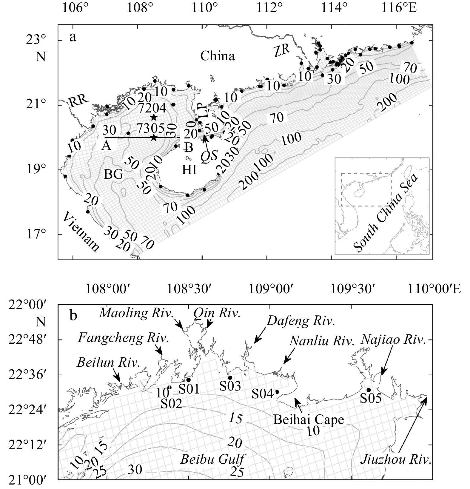
Located in the northwest of the SCS, the Beibu Gulf (BG) is a semi-enclosed shallow bay with an average depth of 42 m (Fig. 1a). Through the southern mouth, the BG connects with the SCS directly, meanwhile, a 30-km wide channel named the Qiongzhou Strait provides another important dynamical bridge for both sides. Except for the Red River being the largest runoff feeding the BG, there are eight rivers located on the top of the bay pouring into the gulf (Fig. 1b), and playing a vital role in the gulf-scale circulation (Ding et al., 2013; Gao et al., 2015). The East Asia Monsoon dominates the whole BG, strong northeast wind prevails in winter while weaker southern wind blows during summer. The BG is rich in varieties of hydrodynamical phenomena, problems associated with the tides (e.g. Shi et al., 2002; Chen et al., 2009; Minh et al., 2014), the circulation (e.g. Wu et al., 2008; Ding et al., 2013), the Beibu Gulf Cold Water Mass (BGCWM, Gao et al., 2014; Chen et al., 2015), the upwelling (Hu et al., 2003; Lü et al., 2008) and the rive plume (Gao et al., 2015) have been broadly and deeply investigated. However, wave-current interaction and its effects on the BG hydrodynamics have been rarely discussed and remains to be elucidated so far.
Figure
1.
The model domain and the topography (a), tide stations are marked as solid dots, 7204 and 7305 Stations of the “China General Oceanographic Survey” are marked as stars, the gray meshes show the model grid (every two grid lines), abbreviations stand for the Beibu Gulf (BG), the Hainan Island (HI), the Qiongzhou Strait (QS), the Leizhou Peninsula (LP), the Red River (RR) and the Zhujiang River (ZR); the top areas of the BG (b), rivers are marked out and the solid dots show the locations of the water-quality buoys placed by the Department of Ocean and Fisheries of Guangxi Zhuang Autonomous Region.
Taking advantage of the wave-current module of the newly developed fully-coupled modeling system COAWST (Warner et al., 2008, 2010), we have discussed roles that wave-current interaction plays in the hydrodynamics of the BG. Dynamics in the surf zone are not included in this study, since the present investigation is dedicated to focus on the inner gulf processes and interactions between the inner gulf and coastal seas. Following this introduction, this paper includes six sections: Section 2 describes the model and its configurations; Section 3 validates the model with multi-observations; Section 4 shows how currents modify waves; Section 5 then presents responses of circulation to wave effects; Section 6 gives explanations for the results in Sections 3, 4 and 5; finally, Section 7 summarizes the present work briefly.
The ROMS is a state-of-the-art regional ocean model which has a wide-range of applications, varying from basin-scale to estuary-scale. We have designed an orthogonal curvilinear grid for the BG, with a total number of grid points being 120×240 (Fig. 1a). The horizontal resolution ranges from 1.3 to 14.9 km, which could make better simulation in the Qiongzhou Strait given that it plays a vital role in dominating the water exchange between two sides (Shi et al., 2002; Wu et al., 2008; Chen et al., 2009; Ding et al., 2013). Twenty levels stretched terrain-following coordinate are applied in the vertical direction, with surface and bottom stretching control parameters theta_s and theta_b set to be 5.0 and 0.4 to better resolve dynamics in these boundary layers (Shchepetkin and McWilliams, 2005). The model bathymetry is interpolated from a hybrid-data based on the General Bathymetric Chart of the Oceans (https://www.bodc.ac.uk/) and the electronic navigation chart data. Besides, the minimum depth is 5 m, which is chosen to ensure stable integration. The vertical mixing coefficient is parameterized by the k-ε submodule of the Generic Length Scale (GLS) turbulence closure scheme (Umlauf and Burchard, 2003; Warner et al., 2005). When waves are absent, quadratic bottom friction is exerted at the bed.
The boundary and initial conditions are both interpolated from the HYbrid Coordinate Ocean Model (HYCOM) GLBa0.08 database (http://hycom.org/hycom). In the BG, the Red River and other eight rivers shown in Fig. 1b are taken into account in the model. Except for that the discharge data of the Najiao River and Jiuzhou River are derived from the corresponding county annals, runoff data of other rivers are given as Gao et al. (2013). Besides, the Zhujiang River discharges at eight river mouths based on Zhao (1990) also work in the model. Tidal harmonic constants of ten tidal constituents (M2, S2, N2, K2, K1, O1, P1, Q1, Mf and Mm) derived from the TPXO7 data are added to the open boundaries as tidal forcing. The 3-hourly air-sea fluxes and sea surface winds at 10 m originated from the ERA-Interim global reanalysis data (https://apps.ecmwf.int/datasets/) are applied to the model as atmosphere forcing. In addition, the BULK_FLUX algorithms based on the Coupled Ocean Atmosphere Response Experiment (COARE) are activated to estimate the net air-sea fluxes and wind stress. The baroclinic time step adopts 60 s with a model-splitting ratio of 30, and the data output frequency is every 3 hours.
2.2
SWAN configurations
SWAN is a third-generation shallow water spectral wave model which could solve wave generation by the wind, wave propagation, dissipation, refraction owing to currents and depth, and nonlinear wave-wave interactions. In the present work, the SWAN model shares the same computational grid and sea surface wind forcing as the ROMS. Twenty-five frequencies ranging from 0.01 to 1 Hz and thirty-six directional bands are used. At the open boundaries, the significant wave height, wave direction and wave period interpolated from the ERA-Interim database are added, aiming to achieve better wave simulation. The integrating time step is 300 s, and the model makes an output every 3 hours.
2.3
COAWST configurations
As described in the 1st section, currents and the free surface elevations are the two dominant currents effects on the waves. In the COAWST, these two effects could be activated via defining CURRENT and WLEV, respectively. Particularly, we define UV_KIRBY according to Kirby and Chen (1989) to take the vertical distribution of the current profile into account when currents are excepted to work.
Then, waves can modulate the currents mainly through three different mechanisms:
(1)Wave-enhanced mixing. Wave breaking injects substantial turbulent kinetic energy to the upper ocean, enhancing the mixing. We employ the TKE_WAVEDISS cooperated with the ZOS_HSIG scheme to reveal this wave effect.
(2)Wave-enhanced bottom stress. The bottom roughness felt by the flow could be enhanced due to turbulence in the wave boundary layer, and this effect is parameterized using the SSW_BBL scheme based on the formula raised by Madsen (1994).
To identify how waves and currents modify each other, and distinguish different roles played by various interactive mechanisms, seven numerical experiments summarized as Table 1 are designed. All experiments are initialized on January 1, 2014 and the simulations last for 210 days. When coupled together, ROMS and SWAN communicate with each other every 600 s. Model outputs of the first 30 days are excluded from the analysis procedure, since the model may be in an adjusting phase during that time.
Table
1.
Model configurations for all numerical experiments
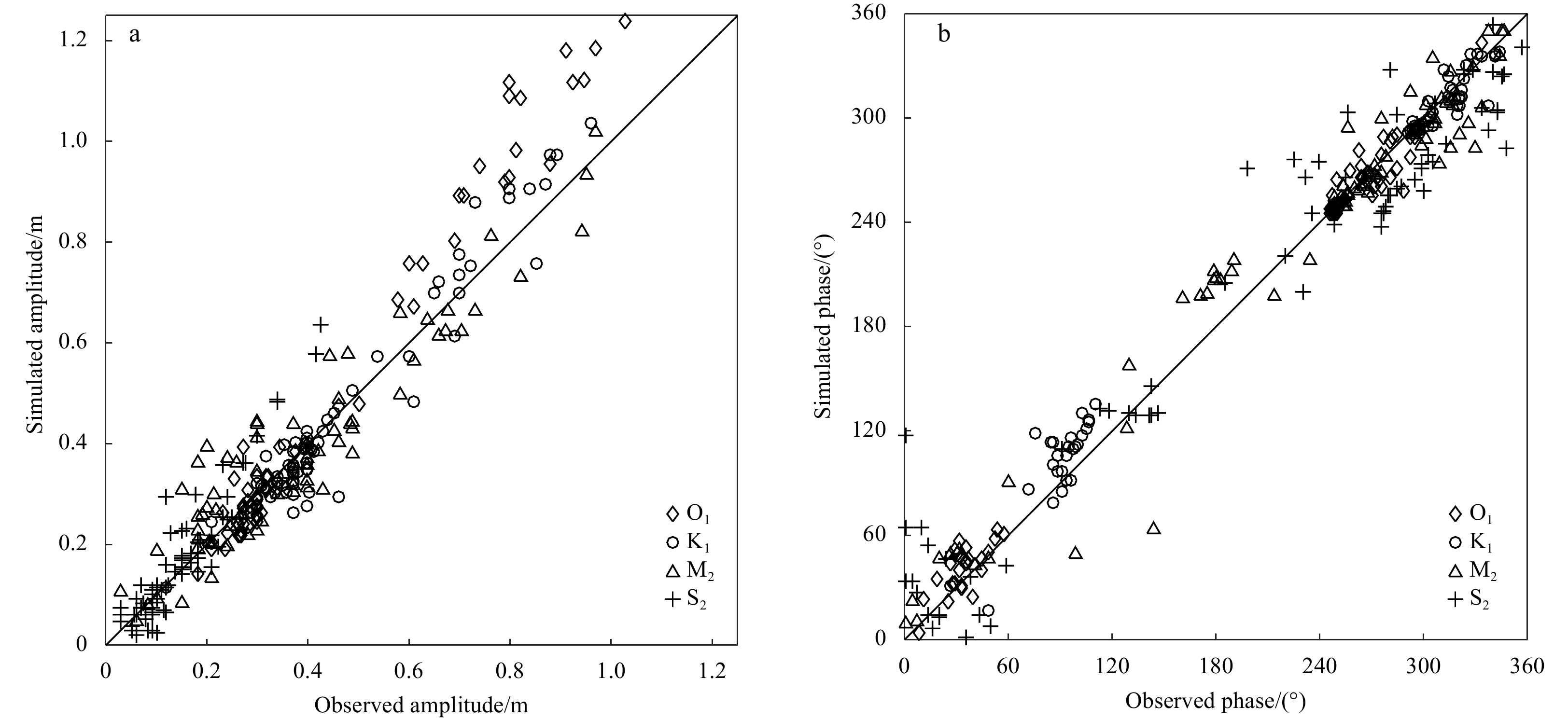
Tides and tidal currents make significant contribution to the circulation and mixing in the BG (e.g. Shi et al., 2002; Chen et al., 2009; Minh et al., 2014). A barotropic-tide model is configured and run for 60 days, the hourly sea surface elevation data during the last 30 days are analyzed using the T_TIDE MATLAB toolbox (Pawlowicz et al., 2002) and the tidal harmonic constants of various tidal constituents are obtained. The model produced tidal harmonic constants for the M2, S2, K1 and O1 tidal constituents are compared with those at 71 tide stations (Fig. 1a), and the comparisons are shown in Fig. 2. Generally, model results show good consistence with observations, the mean absolute errors (MAE) for the M2, S2, K1 and O1 tidal constituents are 6.2, 4.2, 4.3 and 7.1 cm in amplitudes and 15.5º, 28.8º, 10.0º and 7.6º in phases, respectively. Many of the 71 tide stations are located in bays or on small islands, the low-resolution of our model fails to properly describe local topography in these areas and would lead to simulation errors.
Figure
2.
Comparisons of the amplitude (a) and phase (b) between the model and the observation for the M2, S2, K1 and O1 tidal constituents at 71 tide-stations shown in Fig. 1a. The black line shows the linear function y=x.
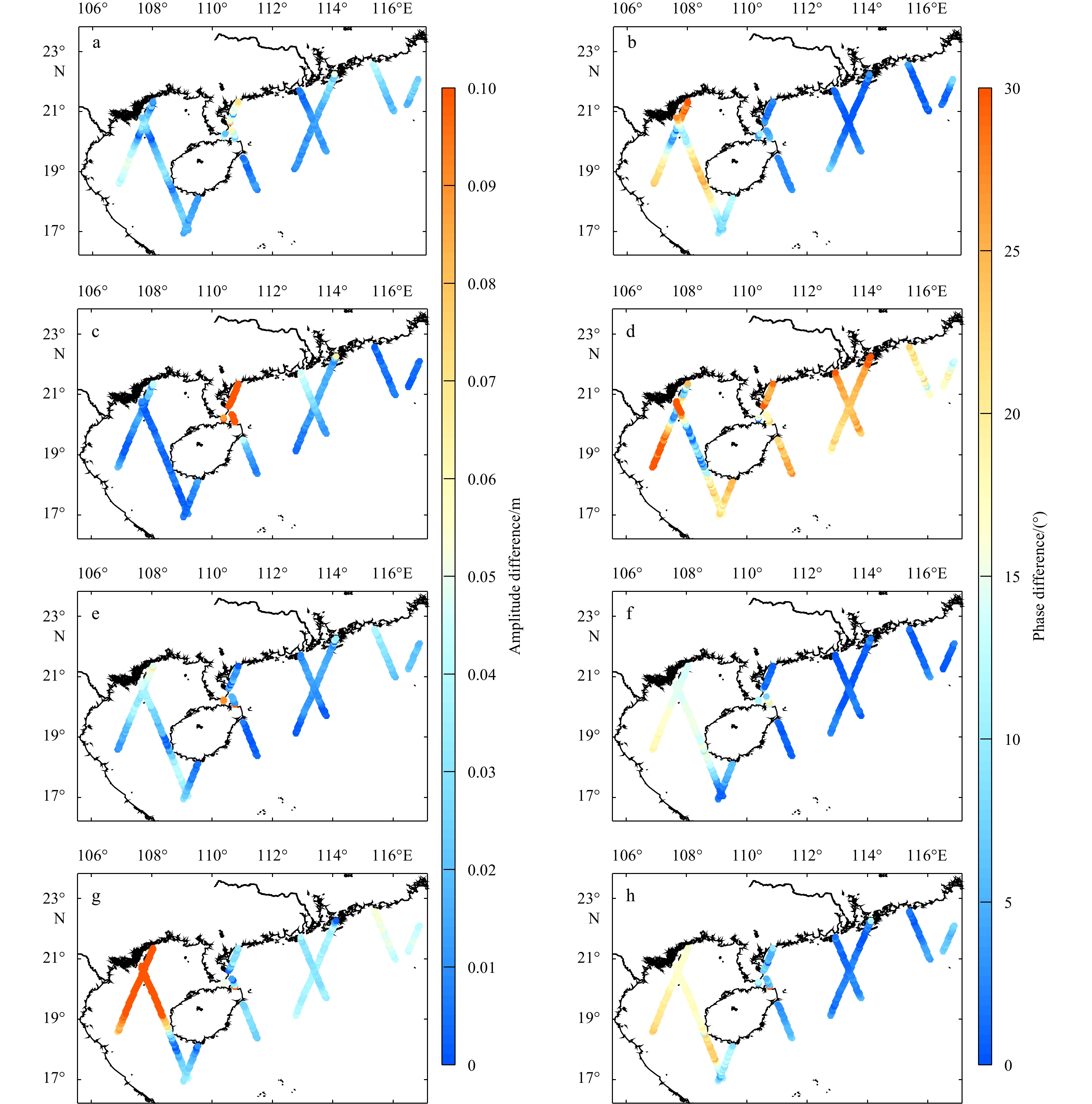
Further, the tidal harmonic constants provided by the CTOH group (Roblou et al., 2007, 2011) which derived from the TOPEX/Poseidon and Jason-1 sea surface height data are also used to check the model tidal performance in the open seas. Jason-1 is the successor of TOPEX/Poseidon and they shared the same orbit, and their ground paths (initial orbit) passing the model domain as well as the simulating errors are shown in Fig. 3. Figure 3 also reveals reasonable model performance, the MAE for the M2, S2, K1 and O1 tidal constituents are 2.1, 2.1, 2.1 and 5.8 cm in amplitudes and 6.6º, 20.6º, 6.1º and 6.1º in phases at 344 measured points, respectively. The better model performance in open seas compared to that in near-shore areas emphasizes the importance of model resolution to a certain extent. Nevertheless, such tidal performance of the model is reasonable and is in favor of further discussion.
Figure
3.
Comparisons of the amplitude (left) and phase (right) between the model and the CTOH data for the M2 (a, b), S2 (c, d), K1 (e, f) and O1 (g, h) tidal constituents.
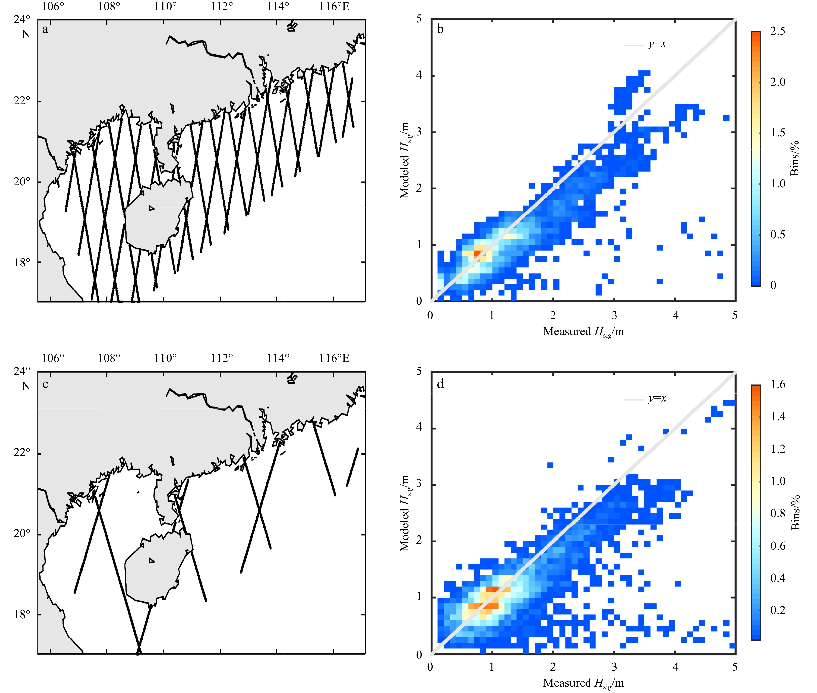
The significant wave height (Hsig) is one of the most representative characteristics of waves, the present study employs the along-track Hsig data derived from the observation of SARAL/ALTIKA and Jason-2 satellites provided by the AVISO to make a validation on the wave module. Only measurements from the Ku-band rather than C-band are used for that the former ones usually have higher accuracy (Olabarrieta et al., 2012). The output of Exp. R2 is validated from 1 February to 29 July, 2014, during which period the total number of comparisons with SARAL/ALTIKA and Jason-2 amounts to 6 640 and 6 958. Comparisons are shown as Figs. 4b and 4d, most of the dots fall into the bins along the linear function y=x and the correlation coefficient (CC) and root mean square error (RMSE) are 0.88, 0.75 and 0.38, 0.50 m for comparisons with SARAL/ALTIKA and Jason-2 respectively, indicating that the modeled Hsig is in fairly good agreement with the observation. Actually, altimetry-satellite-inverted Hsig has errors itself, Durrant et al. (2009) found that the RMSE reached up to 0.2 m when they compared Jason-1 and Envisat inverted Hsig with buoy observations, which may explain part of the errors in the present study.
Figure
4.
Ground tracks of the SARIAL/ALTIKA (a) and Jason-2 (c); scatter diagrams of significant wave height: modeled results (Exp. R2) against the SARIAL/ALTIKA (b) and Jason-2 (d) observations. Scatter diagrams are created by binning the data into 0.1 m bins.
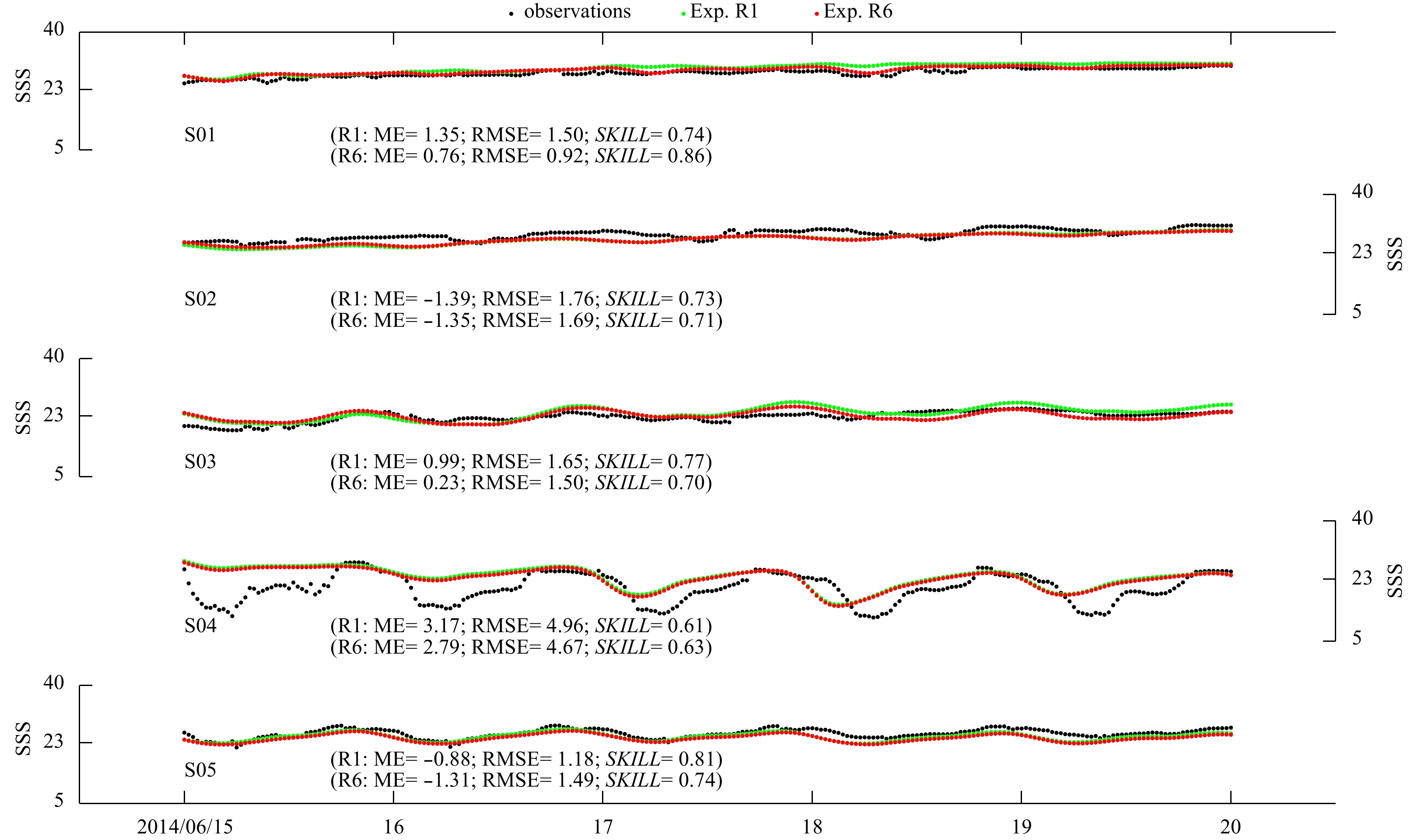
At the top of the BG, a series of rivers discharge into the sea, forming the Guangxi diluted-water plume (hereinafter GXP). In order to monitor the water quality of the Guangxi coastal seas, the Department of Ocean and Fisheries of Guangxi Zhuang Autonomous Region placed a set of water-quality buoy array. The sea surface salinity (SSS) during 15 June to 20 June, 2014 observed by five buoys which located near local river mouths (Fig. 1b) are used in the present validation (for Exps. R1 and R6), and the results are shown in Fig. 5. Except for the mean error (ME) and RMSE, a model skill is also marked in Fig. 5, which is defined as
Figure
5.
Model produced sea surface salinity (SSS) compared against the observations by water-quality buoys at Stations S01–S05 (see Fig. 1b).
where Smod is the modeled salinity, Sobs is the observed salinity, ${\bar S_{obs}}$ is the average of the observations and N is the total number of observations, and higher SKILL value suggests better simulation. Figure 5 reveals that the observed salinity indicates significant tidal-signal in many stations (e.g., Stations S04 and S05). However, low model resolution in those areas makes the model fail to describe the topography accurately, which should account for the unsatisfying variation trends at those stations. Overall, the relative small ME and RMSE and high SKILL at Stations S01-S05 suggest that the model could provide a reasonable simulation of SSS in the GXP area.
3.4
Temperature performance
The MODIS-Aqua sensed Level-2 sea surface temperature (SST, http://oceancolor.gsfc.nasa.gov/) over the northern BG is used to examine that produced by the model (Exp. R1). The MODIS instrument will not work in the presence of clouds, the effective observations during June and July in 2014 are displayed in Figs 6a–e and the corresponding model results are presented in Figs 6f–j, respectively. Figures 6a–f reveal that the simulated SST is in good consistence with the observed one both in varying trend (getting warmer from June to July) and in spatial pattern (higher SST in coastal seas and lower SST in central gulf). In addition, Figs 6k-o show the comparisons for SST along Section AB. Statistically, the RMSE, MAE, ME and CC are 0.64, 0.32, –0.04 and 0.79 for all five comparisons, indicating satisfying model performance. Validation of SST along Section AB is a vital reference which will be used in Section 5.2.
Figure
6.
Comparisons between the MODIS-Aqua Level-2 sensed SST (first row) and the model simulated ones (second row) over the northern Beibu Gulf while sub-figures in the third row show the comparisons along Section AB; note that sub-figures in the same column share the same comparing moment.
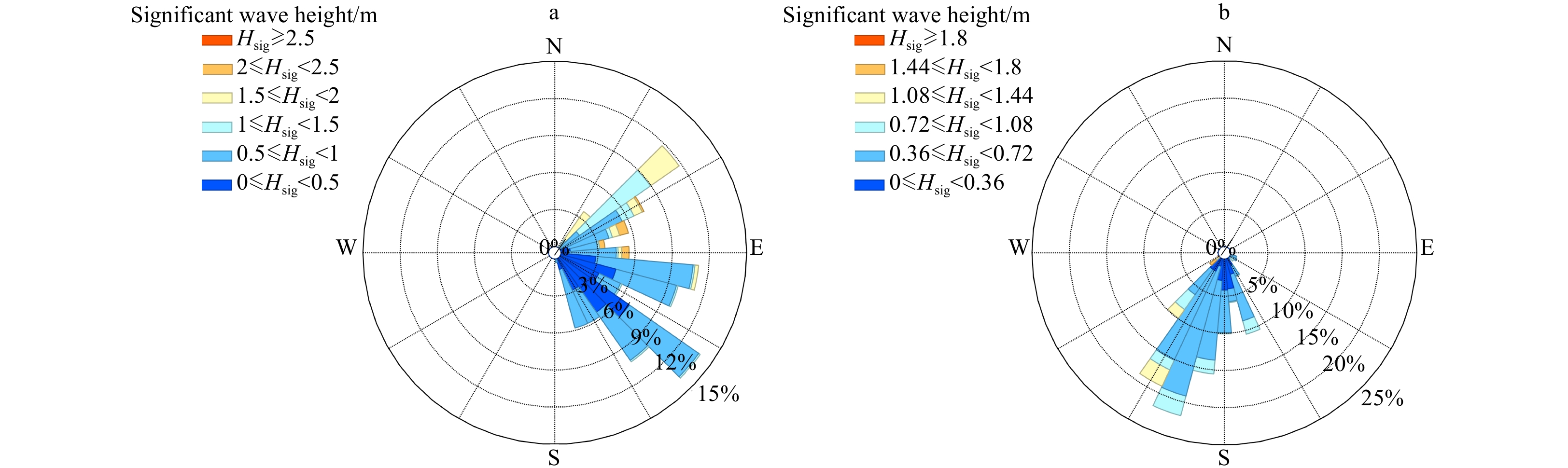
Dominated by the changing monsoon, waves in the BG characterize different features in winter and summer. Wave rose diagrams based on the area-averaged Hsig and wave direction (output of Exp. R2) in the BG (17.5–22.0°N, 105–110°E) are shown as Fig. 7 for winter (February) and summer (July). Figures 7a and b imply that the southeast, east-southeast and northeast are the dominant wave directions in winter, while southwest in summer. The southeast waves in winter and southwest ones in summer are selected as the representative cases for different seasons in the following discussion.
Figure
7.
Wave rose diagrams in winter (a) and summer (b) in the BG based on results of Exp. R2.
The influence of currents variation on the waves is analyzed based on results of Exps. R2, R3 and R4. Comparisons between R2 and R3 suggest minor modulation of the sea level changes exerting on the waves, however, significant modulations were reported in shallow estuaries (e.g. Bolaños et al., 2014).
Except the surface elevations, currents can also modulate wave characteristics via refractions (Olabarrieta et al., 2011). The short-time circulation in the BG features strong diurnal tidal currents signal (Chen et al., 2009), and the velocity could reach up to 2 m/s in the west Hainan Island coastal seas. Therefore, the Hsig difference triggered by the inclusion of currents during a quasi-whole tidal period for both the winter southeast and summer southwest wave cases are presented in Fig. 8 and Fig. 9, respectively.
Figure
8.
The Hsigdifference triggered by the currents (shaded color) under the winter southeast wave, results are derived from the outputs between the Exps. R4 and R3 (R4–R3), values below 5 cm are blanked, the purple arrows show the Hsig and wave direction based on Exp. R2, the green arrows show the surface current vectors based on Exp. R1.
A newly discovered hot spot where currents significantly modify the Hsig is clearly revealed in Fig. 8: in the west and southwest Hainan Island coastal seas, the restriction of the coast makes the current and wave directions being collinear, when they propagate inversely, currents would refract the waves, concentrating the wave rays and focusing wave energy, finally leading to increased Hsig, and vice versa.
The same phenomenon is also indicated in Fig. 9, but, the location of the hot spot is different: it locates on the west and southwest shore of the Hainan Island in winter, but west and northwest in summer. During winter and summer, different prevailing winds generate waves with different directions, therefore, various hot spots occur.
Currents triggered Hsig adjustment could reach up to ±0.2–0.3 m in both summer and winter and, its original value is about 1 m. Thus, currents could increase or decrease local Hsig by 20%–30%, which emphasizes the significance of wave-current interaction in these areas.
5.
Waves effects on currents
5.1
The Beibu Gulf Cold Water Mass (BGCWM)
The BGCWM occurs in summer and locates in 107.5°–109.0°E, 19.5°–21.0°N. It is first reported by the Sino-Vietnam joint marine survey in May 1960. Recently, Chen et al. (2015) established a wave-tide-circulation coupled POM model to make a systematic exploration on the BGCWM. Their results indicated that the BGCWM is a result of the winter-residual-water: in winter, strong mixing cooled the whole water column, then, only the cold water mass in the lower-layer of the bowl-shaped basin could survive when the thermocline developed during spring, finally the winter-residual cold water mass was surrounded by warm water and the BGCWM occurred in summer. Thermal action is the most dominant factor during this process, meanwhile, the terrain and the tidal mixing also play important roles.
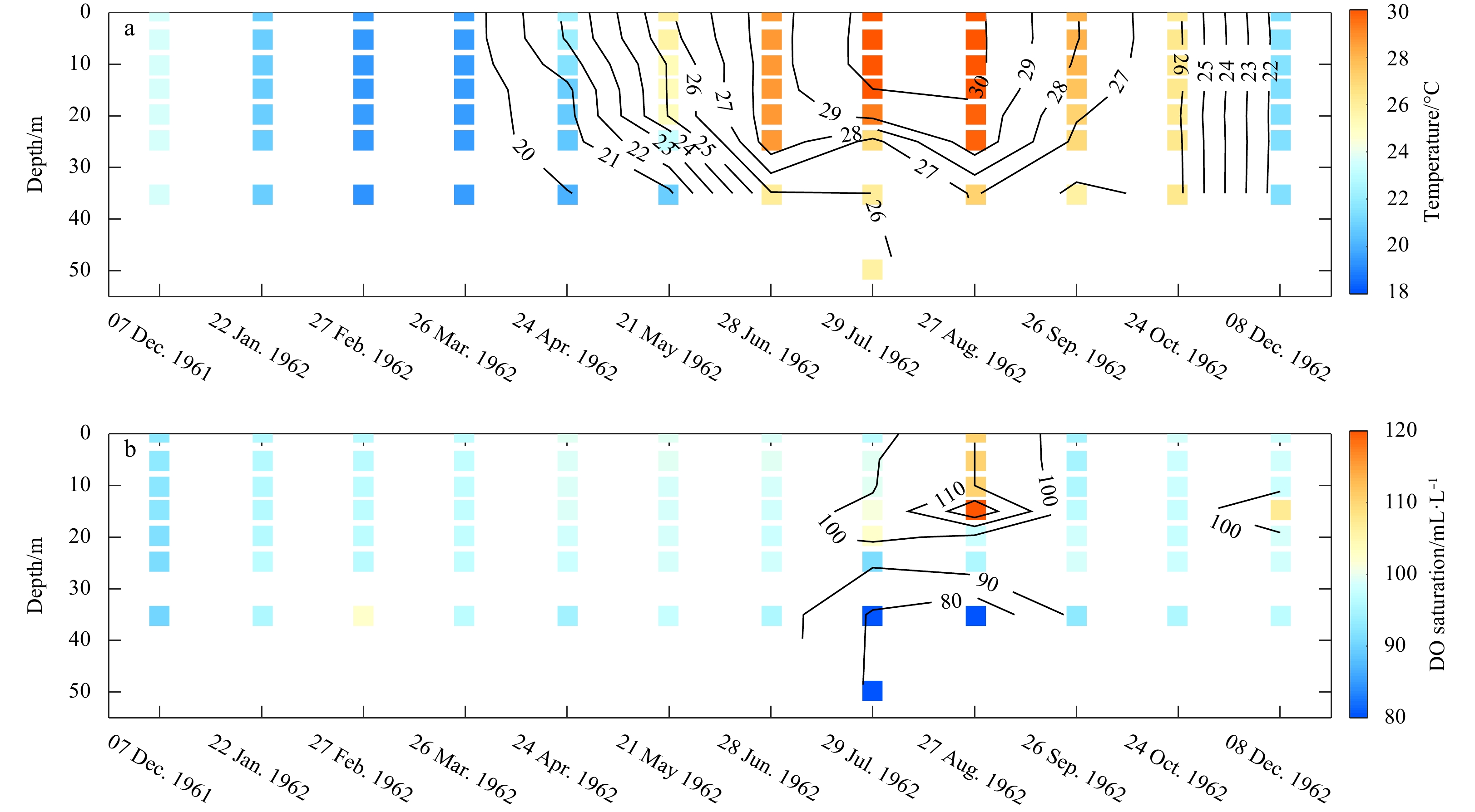
Figure 10 presents the time series of temperature and dissolved oxygen (DO) saturation profiles at Station 7204 (Fig. 1a) during the China General Oceanographic Survey. The time series of temperature profile clearly show the lifecycle of the BGCWM as we described above, and in addition, the gradually decreased DO saturation in the lower layer during the BGCWM developing process is a strong evidence of its residual-water nature.
Figure
10.
Time series of temperature (a) and dissolved oxygen (DO) saturation (b) profiles at Station 7204 (Fig. 1a) during the China General Oceanographic Survey.
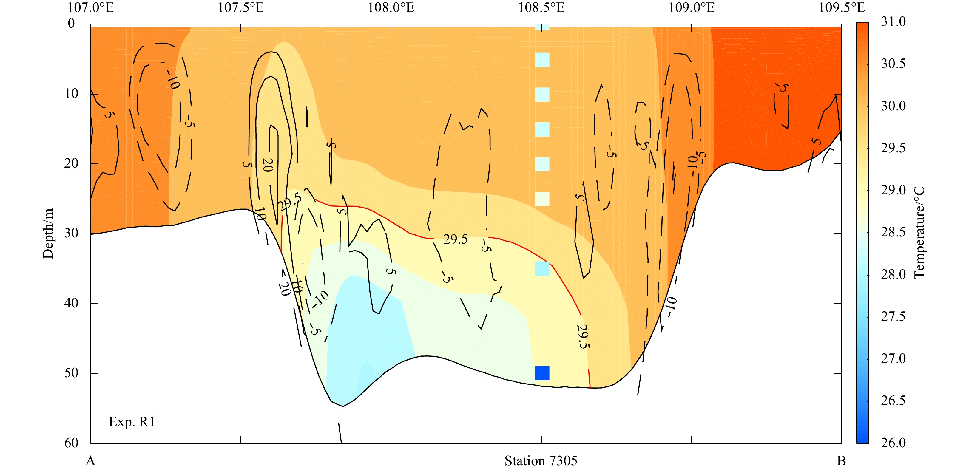
The model could produce the BGCWM phenomenon as shown in Fig. 11. During the study year, the core intensity of the BGCWM is about 28°C, which is much weaker than that observed at Station 7305 in 1962 (26°C, Fig. 11). However, section 3.4 suggests that the model makes reasonable simulation of the SST along section AB. Taking the SST as a reference, the significant discrepancy here indicates that the BGCWM may characterize long-term variations rather than model errors.
Figure
11.
Monthly averaged temperature along Section AB (Fig. 1a) during June 2014; solid-black lines indicate upward vertical velocity while dashed lines indicate downward motion (10–6 m/s); the scattered squares show the temperature profile observed at Station 7305 (Fig. 1a) in June 1962 during the China General Oceanographic Survey, all the results are based on Exp. R1.
Figure 11 reveals that the core of the BGCWM lies in the left canyon. On one hand, the left canyon is deeper than the right one, which could provide better shelter for the BGCWM. On the other hand, the right part of the bowl-shaped basin locates near the west entrance of the Qiongzhou Strait (Fig. 1a), where the tidal mixing is rather intense (Hu et al., 2003), therefore, the east part of the cold water mass would be eroded faster than the west part. As a result, the temperature gradient induced pressure gradient force triggers an upwelling-like motion along the west slope of the basin, but no similar phenomenon occurs on the opposite side.
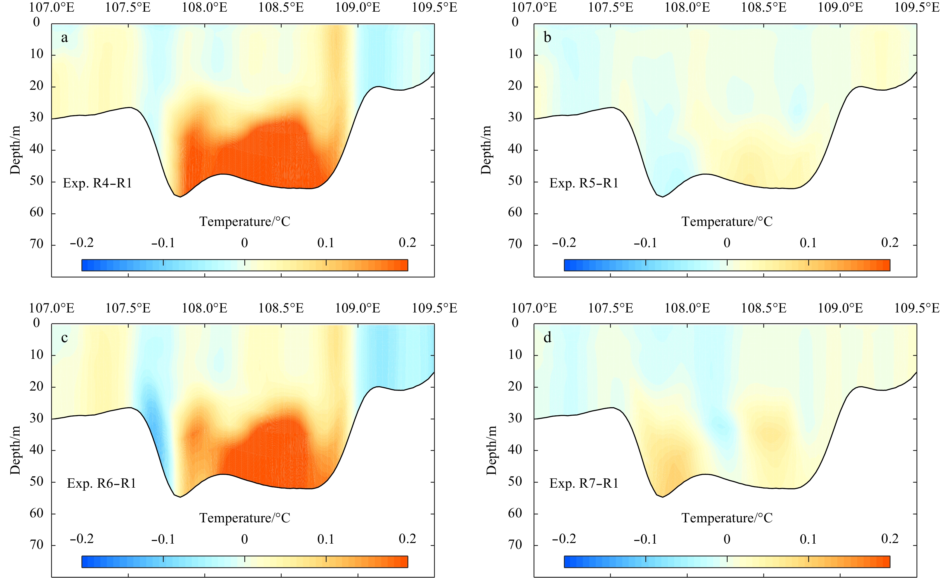
Currents’ responses to different wave effects could be analyzed by checking the difference between different numerical experiments. Figures 12b, c and d show the temperature adjustment owing to wave enhanced mixing, wave enhanced bottom friction and 3-D wave forces, respectively. Compared to the wave enhanced bottom friction which decreases the BGCWM intensity by about 0.2°C, the other two wave effects only induce much weaker adjustment. Figure 12a displays the temperature response when three wave effects cooperate together, which approximately equals to the linear superposition of Figs 12b, c and d, suggesting relatively weak nonlinear interaction between different wave effects (Rong et al., 2014).
Figure
12.
Temperature difference along Section AB between numerical experiments R4 and R1 (a), R5 and R1 (b), R6 and R1 (c), R7 and R1 (d).
Based on the monthly averaged model output during June 2014, the sea surface salinity (SSS) and depth-averaged horizontal velocity in the top BG areas are shown as Fig. 13, in which remarkable diluted-water plume could be found. The background large scale circulation is cyclonic type, which would transport the diluted-water to the downstream towards the central BG.
Figure
13.
The sea surface salinity superposed by the depth-averaged velocity in the top BG areas, the data is based on the monthly averaged outputs of Exp. R1 during June 2014.
The response of SSS field to wave enhanced mixing, wave enhanced bottom friction and wave forces are presented in Figs 14b, c and d, respectively. Again, wave enhanced mixing and wave forces could lead to SSS change, but too weak compared to that induced by wave enhanced bottom stress. The inclusion of wave enhanced bottom boundary layer decreases the SSS near the river mouths while increases the SSS in the downstream areas, and the adjustment could reach up to 1 PSU. Similar with the BGCWM case, weak nonlinear interactions among different wave effects are also indicated according to Figs 14a-d.
Figure
14.
The sea surface salinity difference in the top BG areas between numerical experiments R4 and R1 (a), R5 and R1 (b), R6 and R1 (c), R7 and R1 (d).
A section named CD shown as gray line in Fig. 14a is used to reveal the salinity change in the vertical direction, and different wave effects induced salinity modulations along section CD are shown in Fig. 15. The wave enhanced mixing and waves forces still lead to minor salinity change in the vertical direction as shown in Figs 15b and d. However, Fig. 15c reveals that the salinity decreases from surface to bottom in the near-fields (21.5°–21.6°N), and increases in the whole water column in the adjacent seas (21.2°–21.4°N), then increases in the upper 10 m layers in the far-fields (20.5°–20.9°N). Figures 14 and 15 suggest that the diluted-water is redistributed when waves are involved in.
Figure
15.
The salinity difference along Section CD between numerical experiments R4 and R1 (a), R5 and R1 (b), R6 and R1 (c), R7 and R1 (d).
Section 5.1 reveals that the inclusion of wave effects suppressed the intensity of the BGCWM, and wave enhanced bottom shear stress is found to be the dominant factor during this process according to the diagnostic numerical experiments. Temperature dynamics in the BGCWM region is further investigated via the model diagnostic of the heat equation:
where the term on the left-hand-side is the time rate of change for temperature (RATE), and on the right-hand-side, they are the horizontal advection term (HADV), the vertical advection term (VADV) and the vertical diffusivity term (VDIFF), respectively. Actually, the horizontal diffusivity term is also included in the model diagnostics, but its magnitude is negligible compared to other terms.
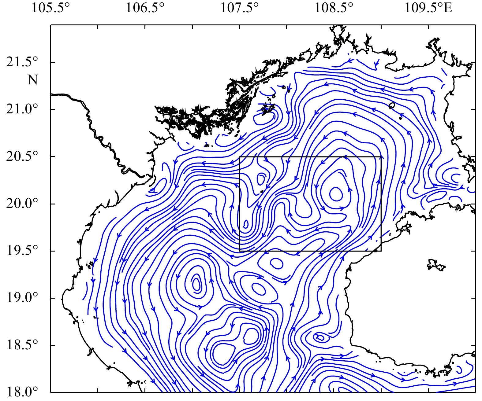
Based on Fig. 11, the BGCWM locates in the bowl-shaped basin where deeper than 20 m. Therefore, all temperature diagnostic terms in Eq.(2) are integrated over the BGCWM area (black box in Fig. 16) horizontally and below 20 m vertically throughout the whole June, 2014. The results are displayed in Table 2.
Figure
16.
The streamline of depth-averaged flow during June, 2014 based on the monthly-averaged data from Exp. R1, the black box shows the BGCWM domain.
During June, the BGCWM has warmed by about 0.55°C based on Table 2, indicating that the BGCWM is getting eroded. The vertical advection and diffusivity both present positive values, that is, these two terms play a role as facilitating exchange between the warm upper-layer water and the cold BGCWM water, finally making the BGCWM become warmer. However, the BGCWM is maintained by the horizontal advection effect for that this term is negative.
Figure 16 displays the streamline of depth-averaged flow during June, 2014 based on the monthly-averaged data from Exp. R1. Clearly, the BGCWM is connected to the waters in the southern gulf by the gulf-scale cyclonic circulation (Wu et al., 2008; Ding et al., 2013), which is a strong indicator that the BGCWM is under the influence of the water transport from the southern gulf. Besides, Table 2 also suggests that only the negative HADV benefits preserving the BGCWM during the summer. Although the VADV in Exp. R4 and R6 are weaker than other cases, it should be a passive adjustment for matching and balancing the change of HADV. Therefore, it reminds us that the background circulation may have changed with the inclusion of wave enhanced bottom stress.
Taking results of Exp. R1 as a reference, Fig. 17 displays the differences of monthly mean depth-averaged flow against Exps. R4 (a), R5 (b), R6 (c) and R7(d) during June, 2014. At the entrance where the BGCWM is connected with the southern gulf, the background circulation is significantly suppressed by wave enhanced bottom stress as shown in Fig. 17c. The water transport through section EF (Fig. 17) which lies on the southern edge of the BGCWM is calculated. According to the intensity of the BGCWM core, we define <29.5°C as the criteria for benefitting the maintenance of the BGCWM, the water transport (<29.5°C) through section EF are shown in Table 3. Table 3 reveals that the cold water supplement transported from the southern gulf to the BGCWM region is decreased by wave enhanced bottom stress, which is consistent with the weakened background circulation. In addition, the weakened circulation-bridge between the BGCWM and the southern gulf locates on the 30–50 m isobaths, just being the depth where the BGCWM core exists. It means that the water transport through this entrance could exert direct influence on the BGCWM, which makes a further explanation why the BGCWM intensity is sensitive to wave enhanced bottom shear stress.
Figure
17.
Difference of monthly mean depth-averaged flow between Exp. R4 (a), R5 (b), R6 (c), R7 (d) and the R1 during June 2014. Arrows show changes of the current vectors, colors display changes of the magnitude for the current, with positive value indicating the current is enhanced and vice versa. Black box shows the BGCWM domain and the red line shows the location of Section EF.
As revealed in Section 5.2, the salinity decreases in the near-field of the river estuary but increases in the downstream seas when wave enhanced bottom stress works. The fresh water thickness defined as the integral of fresh water anomaly over the vertical water column is calculated via:
where S0 is the reference salinity, chosen to be 36 PSU in the present work, S is the salinity in different layers of the water column. Different reference salinity leads to different hf, but it won’t affect the discussion since we focus on the changes of freshwater thickness. The freshwater thickness difference owing to different wave effects is in good consistence with what reveals in Fig.14 (not shown), which implies that the fresh water amount increases owing to the inclusion of wave enhanced bottom stress in the near-field of river estuaries, while decreases in the downstream areas. Again, this is an indicator that the transport process of the GXP is modulated, that is, the background circulation should be changed.
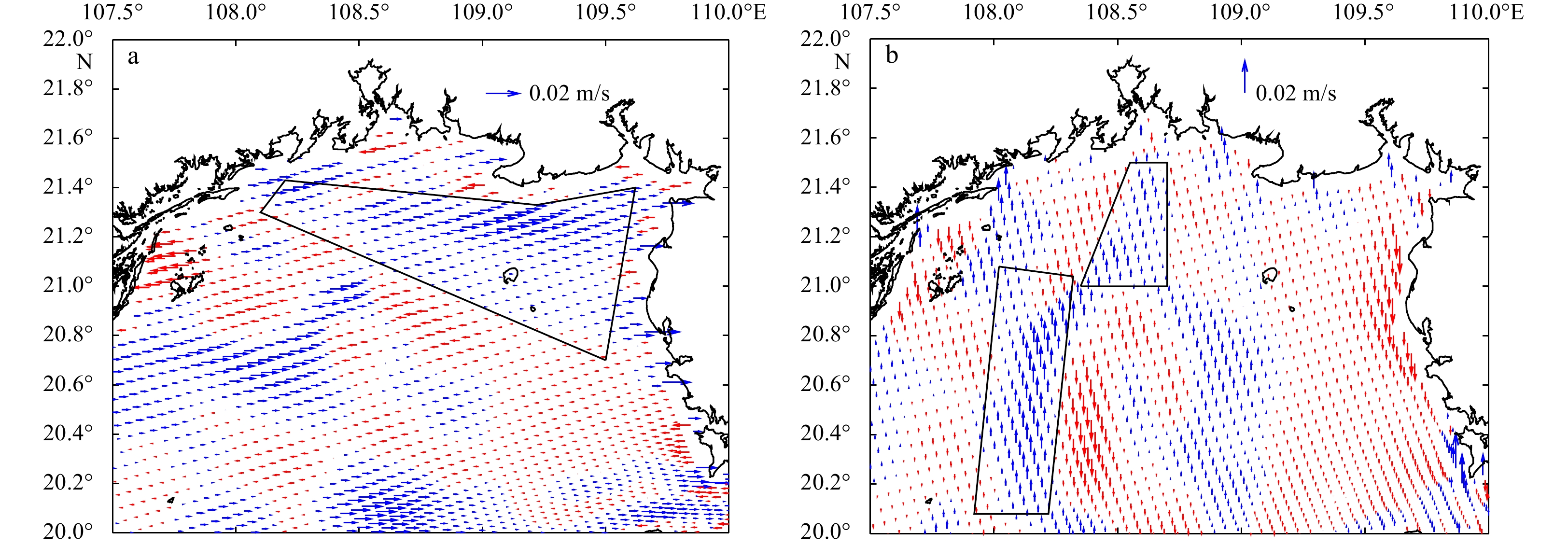
After poured into the seas, the GXP would be transported to the downstream toward west and south under the carrying of the northern-part of the basin-scale circulation (Fig. 13). Figure 18 shows the differences of eastward and northward current components owing to the wave enhanced bottom stress. It clearly implies that this wave effect makes a reduction on the background circulation and retards the transport of the GXP to the downstream. Therefore, more fresh water would be trapped in the near-field and less transported to the far-field, leading to lower salinity near the river mouth but higher salinity downstream. Rong et al. (2014) and Gong et al. (2018) also have reported similar phenomena when they investigated the responses of river plume to wave effects.
Figure
18.
Differences of eastward (a) and northward (b) current components of the monthly mean depth-averaged flow in June 2014 between Exps. R6 and R1 (R6–R1), where blue arrows indicating negative values and red arrows for positive ones.
Wave-current interaction model based on the COAWST modeling system has been configured for the BG to investigate effects of wave-current interaction on the local hydrodynamics. A set of diagnostic numerical experiments are designed to distinguish different roles played by different wave-current interactive physical mechanisms. Validated by multi-originate observations, the model simulated variables show reasonable consistence with the observed ones.
A newly-founded hot spot located on the west coastal seas of the Hainan Island where currents could trigger 20%–30% modification of the significant wave height is reported. On one hand, the wave- and current-directions tend to be collinear under the restriction of the topography, on the other hand, tidal currents are intense there. Thus, the counter-flowing currents could effectively concentrate wave energy, finally leading to increased significant wave height, and vice versa.
The Beibu Gulf Cold Water Mass (BGCWM) and the Guangxi diluted-water Plume (GXP) are the two typical cases showing how wave effects modulate currents in the BG. The wave enhanced bottom stress retards the near-shore part of the gulf-scale cyclonic-circulation in summer, leading to less cold water supplement from the southern gulf to the BGCWM area and more fresh water trapped in the river mouth area at the top of the BG, therefore, the intensity of the BGCWM and the distribution of the GXP are modulated.
However, the improvement of the model skill owing to different wave-current interactive effects has not been well discussed in the present work. This is mainly due to the lack of in-situ observations. Few satellite-based significant wave height observations in the west Hainan Island coastal seas makes it difficult to validate the hot spot where waves are modulated significantly by the currents, though it makes sense theoretically. Actually, the mean error of the salinity simulated by the model with inclusion of wave enhanced bottom friction is improved based on Fig. 5, which proves that waves could trap more fresh water locally.
Compared to the wave enhanced bottom stress, effects of wave enhanced mixing and wave forces are weak and chaotic in the BG, drawing less concern in the present study. Different with our results, investigation of Rong et al. (2014) proposed that wave-enhanced mixing and 3-D wave forces could both play vital role in altering the Mississippi–Atchafalaya river plume dynamics on the Texas–Louisiana shelf. This should be due to the differences of the topography (shallow in present work but much deeper in Rong et al., 2014) and discharge amount (weak in present work but very vigorous in Rong et al., 2014). In the shallow Zhujiang River Estuary, Gong et al. (2018) suggested that wave enhanced bottom friction is the most important wave process influencing the river plume near the river mouths, this is quite similar with present study. Previous studies have emphasized the importance of wave-enhanced surface wind stress for the circulation (e.g. Xie et al., 2001; Niu and Xia, 2017; Gong et al., 2018) and the vital role of surf zone dynamics (e.g. Olabarrieta et al., 2011; Kumar et al., 2012), but these effects are not introduced into the present investigation. In the future, it would be interesting to explore influences of these two unconsidered wave effects on the hydrodynamics in the BG. Meanwhile, wave-current interaction during storm events in the BG would also be an interesting topic.
Acknowledgements
We appreciate the editors and anonymous reviewers for their constructive suggestions which lead to substantial improvement of the manuscript. Peng Bai thanks John C. Warner and Zengrui Rong sincerely for their generous and great assistance in building up the COAWST model.
Beardsley R C, Chen Changsheng, Xu Qichun. 2013. Coastal flooding in Scituate (MA): a FVCOM study of the 27 December 2010 nor’easter. Journal of Geophysical Research: Oceans, 118(11): 6030–6045. doi: 10.1002/2013JC008862
[2]
Bolaños R, Brown J M, Souza A J. 2014. Wave-current interactions in a tide dominated estuary. Continental Shelf Research, 87: 109–123. doi: 10.1016/j.csr.2014.05.009
[3]
Booij N, Ris R C, Holthuijsen L H. 1999. A third-generation wave model for coastal regions: 1. Model description and validation. Journal of Geophysical Research: Oceans, 104(C4): 7649–7666
[4]
Carniel S, Warner J C, Chiggiato J, et al. 2009. Investigating the impact of surface wave breaking on modeling the trajectories of drifters in the northern Adriatic Sea during a wind-storm event. Ocean Modelling, 30(2–3): 225–239. doi: 10.1016/j.ocemod.2009.07.001
[5]
Chen Changlin, Li Peiliang, Shi Maochong, et al. 2009. Numerical study of the tides and residual currents in the Qiongzhou Strait. Chinese Journal of Oceanology and Limnology, 27(4): 931–942. doi: 10.1007/s00343-009-9193-0
[6]
Chen Zhenhua, Qiao Fangli, Xia Changshui, et al. 2015. The numerical investigation of seasonal variation of the cold water mass in the Beibu Gulf and its mechanisms. Acta Oceanologica Sinica, 34(1): 44–54. doi: 10.1007/s13131-015-0595-x
[7]
Ding Yang, Chen Changsheng, Beardsley R C, et al. 2013. Observational and model studies of the circulation in the Gulf of Tonkin, South China Sea. Journal of Geophysical Research: Oceans, 118(12): 6495–6510. doi: 10.1002/2013JC009455
[8]
Durrant T H, Greenslade D J M, Simmonds I. 2009. Validation of Jason-1 and Envisat remotely sensed wave heights. Journal of Atmospheric and Oceanic Technology, 26(1): 123–134. doi: 10.1175/2008JTECHO598.1
[9]
Fan Yalin, Ginis I, Hara T, et al. 2009. Numerical simulations and observations of surface wave fields under an extreme tropical cyclone. Journal of Physical Oceanography, 39(9): 2097–2116. doi: 10.1175/2009JPO4224.1
[10]
Gao Jingsong, Chen Bo, Shi Maochong. 2015. Summer circulation structure and formation mechanism in the Beibu Gulf. Science China Earth Sciences, 58(2): 286–299. doi: 10.1007/s11430-014-4916-2
[11]
Gao Jingsong, Shi Maochong, Chen Bo, et al. 2014. Responses of the circulation and water mass in the Beibu Gulf to the seasonal forcing regimes. Acta Oceanologica Sinica, 33(7): 1–11. doi: 10.1007/s13131-014-0506-6
[12]
Gao Jingsong, Xue Huijie, Chai Fei, et al. 2013. Modeling the circulation in the gulf of Tonkin, South China Sea. Ocean Dynamics, 63(8): 979–993. doi: 10.1007/s10236-013-0636-y
[13]
Gong Wenping, Lin Zhongyuan, Chen Yunzhen, et al. 2018. Effect of waves on the dispersal of the Pearl River plume in winter. Journal of Marine Systems, 186: 47–67. doi: 10.1016/j.jmarsys.2018.05.003
[14]
Haidvogel D B, Arango H G, Hedstrom K, et al. 2000. Model evaluation experiments in the North Atlantic basin: simulations in nonlinear terrain-following coordinates. Dynamics of Atmospheres and Oceans, 32(3–4): 239–281. doi: 10.1016/S0377-0265(00)00049-X
[15]
Hu Jianyu, Kawamura H, Tang Danling. 2003. Tidal front around the Hainan Island, northwest of the South China Sea. Journal of Geophysical Research: Oceans, 108(C11): 3342. doi: 10.1029/2003JC001883
[16]
Jacob R, Larson J, Ong E. 2005. M×N communication and parallel interpolation in Community Climate System Model Version 3 using the model coupling toolkit. The International Journal of High Performance Computing Applications, 19(3): 293–307. doi: 10.1177/1094342005056116
[17]
Kirby J T, Chen T M. 1989. Surface waves on vertically sheared flows: approximate dispersion relations. Journal of Geophysical Research: Oceans, 94(C1): 1013–1027. doi: 10.1029/JC094iC01p01013
[18]
Kumar N, Voulgaris G, Warner J C, et al. 2012. Implementation of the vortex force formalism in the coupled ocean-atmosphere-wave-sediment transport (COAWST) modeling system for inner shelf and surf zone applications. Ocean Modelling, 47: 65–95. doi: 10.1016/j.ocemod.2012.01.003
[19]
Larson J, Jacob, R, Ong, E. 2004. The Model Coupling Toolkit: A New Fortran90 Toolkit for Building Multiphysics Parallel Coupled Models. Preprint ANL/MCSP1208–1204. Mathematics and Computer Science Division, Argonne National Laboratory, 25
[20]
Longuet-Higgins M S. 1970. Longshore currents generated by obliquely incident sea waves: 2. Journal of Geophysical Research, 75(33): 6790–6801. doi: 10.1029/JC075i033p06790
[21]
Longuet-Higgins M S, Stewart R W. 1962. Radiation stress and mass transport in gravity waves, with application to ‘surf beats’. Journal of Fluid Mechanics, 13(4): 481–504. doi: 10.1017/S0022112062000877
[22]
Lü Xingang, Qiao Fangli, Wang Guansuo, et al. 2008. Upwelling off the west coast of Hainan Island in summer: Its detection and mechanisms. Geophysical Research Letters, 35(2): L02604
[23]
Madsen O S. 1994. Spectral wave–current bottom boundary layer flows. In: Proceedings of the 24th International Conference on Coastal Engineering. Kobe, Japan: American Society of Civil Engineers, 384–398
[24]
McWilliams J C, Restrepo J M, Lane E M. 2004. An asymptotic theory for the interaction of waves and currents in coastal waters. Journal of Fluid Mechanics, 511: 135–178. doi: 10.1017/S0022112004009358
[25]
Minh N N, Patrick M, Florent L, et al. 2014. Tidal characteristics of the gulf of Tonkin. Continental Shelf Research, 91: 37–56. doi: 10.1016/j.csr.2014.08.003
[26]
Niu Qianru, Xia Meng. 2017. The role of wave-current interaction in Lake Erie’s seasonal and episodic dynamics. Journal of Geophysical Research: Oceans, 122(9): 7291–7311. doi: 10.1002/2017JC012934
[27]
Olabarrieta M, Warner J C, Armstrong B, et al. 2012. Ocean-atmosphere dynamics during Hurricane Ida and Nor'Ida: An application of the coupled ocean-atmosphere-wave-sediment transport (COAWST) modeling system. Ocean Modelling, 43: 112–137
[28]
Olabarrieta M, Warner J C, Kumar N. 2011. Wave-current interaction in Willapa Bay. Journal of Geophysical Research: Oceans, 116(C12): C12014. doi: 10.1029/2011JC007387
[29]
Osuna P, Monbaliu J. 2004. Wave-current interaction in the Southern North Sea. Journal of Marine Systems, 52(1–4): 65–87. doi: 10.1016/j.jmarsys.2004.03.002
[30]
Pawlowicz R, Beardsley B, Lentz S. 2002. Classical tidal harmonic analysis including error estimates in MATLAB using T_TIDE. Computers & Geosciences, 28(8): 929–937
[31]
Pleskachevsky A, Eppel D P, Kapitza H. 2009. Interaction of waves, currents and tides, and wave-energy impact on the beach area of Sylt Island. Ocean Dynamics, 59(3): 451–461. doi: 10.1007/s10236-008-0174-1
[32]
Qiao Fangli, Xia Changshui, Shi Jianwei, et al. 2004. Seasonal variability of thermocline in the Yellow Sea. Chinese Journal of Oceanology and Limnology, 22(3): 299–305. doi: 10.1007/BF02842563
[33]
Ris R C, Holthuijsen L H, Booij N. 1999. A third-generation wave model for coastal regions: 2. Verification. Journal of Geophysical Research: Oceans, 104(C4): 7667–7681. doi: 10.1029/1998JC900123
[34]
Roblou L, Lamouroux J, Bouffard J, et al. 2011. Post-processing altimeter data towards coastal applications and integration into coastal models. In: Vignudelli S, Kostianoy A G, Cipollini P, et al, eds. Coastal Altimetry. Berlin, Heidelberg: Springer, 217–246
[35]
Roblou L, Lyard F, Le Henaff M, et al. 2007. X-TRACK, a new processing tool for altimetry in coastal oceans. In: Proceedings of 2007 IEEE International Geoscience and Remote Sensing Symposium. Barcelona: IEEE, 5129–5133
[36]
Rong Zengrui, Hetland R D, Zhang Wenxia, et al. 2014. Current-wave interaction in the Mississippi-Atchafalaya river plume on the Texas-Louisiana shelf. Ocean Modelling, 84: 67–83. doi: 10.1016/j.ocemod.2014.09.008
[37]
Shchepetkin A F, McWilliams J C. 2005. The Regional Oceanic Modeling System (ROMS): a split-explicit, free-surface, topography-following-coordinate oceanic model. Ocean Modelling, 9(4): 347–404. doi: 10.1016/j.ocemod.2004.08.002
[38]
Shi Maochong, Chen Changsheng, Xu Qichun, et al. 2002. The role of Qiongzhou Strait in the seasonal variation of the South China Sea circulation. Journal of Physical Oceanography, 32(1): 103–121. doi: 10.1175/1520-0485(2002)032<0103:TROQSI>2.0.CO;2
[39]
Skamarock W C, Klemp J B, Dudhia J, et al. 2005. A description of the advanced research WRF version 2. NCAR Technical Note, NCAR/TN-468+STR
[40]
Svendsen I A. 1984. Mass flux and undertow in a surf zone. Coastal Engineering, 8(4): 347–365. doi: 10.1016/0378-3839(84)90030-9
[41]
Uchiyama Y, McWilliams J C, Shchepetkin A F. 2010. Wave-current interaction in an oceanic circulation model with a vortex-force formalism: application to the surf zone. Ocean Modelling, 34(1–2): 16–35. doi: 10.1016/j.ocemod.2010.04.002
[42]
Umlauf L, Burchard H. 2003. A generic length-scale equation for geophysical turbulence models. Journal of Marine Research, 61(2): 235–265. doi: 10.1357/002224003322005087
Warner J C, Armstrong B, He Ruoying, et al. 2010. Development of a coupled ocean-atmosphere-wave-sediment transport (COAWST) modeling system. Ocean Modelling, 35(3): 230–244. doi: 10.1016/j.ocemod.2010.07.010
[45]
Warner J C, Sherwood C R, Arango H G, et al. 2005. Performance of four turbulence closure models implemented using a generic length scale method. Ocean Modelling, 8(1–2): 81–113. doi: 10.1016/j.ocemod.2003.12.003
[46]
Warner J C, Sherwood C R, Signell R P, et al. 2008. Development of a three-dimensional, regional, coupled wave, current, and sediment-transport model. Computers & Geosciences, 34(10): 1284–1306
[47]
Wolf J, Prandle D. 1999. Some observations of wave-current interaction. Coastal Engineering, 37(3–4): 471–485. doi: 10.1016/S0378-3839(99)00039-3
[48]
Wu Dexing, Wang Yue, Lin Xiaopei, et al. 2008. On the mechanism of the cyclonic circulation in the Gulf of Tonkin in the summer. Journal of Geophysical Research: Oceans, 113(C9): C09029
[49]
Xie Lian, Wu Kejian, Pietrafesa L, et al. 2001. A numerical study of wave-current interaction through surface and bottom stresses: Wind-driven circulation in the South Atlantic Bight under uniform winds. Journal of Geophysical Research: Oceans, 106(C8): 16841–16855. doi: 10.1029/2000JC000292
[50]
Yang Yongzeng, Qiao Fangli, Xia Changshui, et al. 2004. Wave-induced mixing in the Yellow Sea. Chinese Journal of Oceanology and Limnology, 22(3): 322–326. doi: 10.1007/BF02842566
[51]
Zhang Xuefeng, Han Guijun, Wang Dongxiao, et al. 2011. Effect of surface wave breaking on the surface boundary layer of temperature in the Yellow sea in summer. Ocean Modelling, 38(3–4): 267–279. doi: 10.1016/j.ocemod.2011.04.006
[52]
Zhang Chen, Hou Yijun, Li Jian. 2018. Wave-current interaction during Typhoon Nuri (2008) and Hagupit (2008): an application of the coupled ocean-wave modeling system in the northern South China Sea. Journal of Oceanology and Limnology, 36(3): 663–675. doi: 10.1007/s00343-018-6088-y
[53]
Zhao Huanting. 1990. The Evolution of the Pearl River Estuary (in Chinese). Beijing: China Ocean Press, 1–357
[54]
Zhao Biao, Qiao Fangli, Cavaleri L, et al. 2017. Sensitivity of typhoon modeling to surface waves and rainfall. Journal of Geophysical Research: Oceans, 122(3): 1702–1723. doi: 10.1002/2016JC012262
Bingchen Liang, Xianghe Zhang, Zhuxiao Shao, et al. Response of wave energy to tidal influence along the coast of Shandong Peninsula, China. Energy, 2025, 320: 135266. doi:10.1016/j.energy.2025.135266
2.
Haoyu Li, Kai Wei. Effect of wave–current–surge interactions on simulated wave conditions in a strait via an optimal WRF typhoon model. Ocean Engineering, 2025, 326: 120962. doi:10.1016/j.oceaneng.2025.120962
3.
Fang Liu, Ruijie Zhang, Haolan Li, et al. Distribution and adsorption-desorption of organophosphate esters from land to sea in the sediments of the Beibu Gulf, South China Sea: Impact of seagoing river input. Science of The Total Environment, 2024, 917: 170359. doi:10.1016/j.scitotenv.2024.170359
4.
Chaoshuai Wei, Yinghui Wang, Ruijie Zhang, et al. Spatiotemporal distribution and potential risks of antibiotics in coastal water of Beibu Gulf, South China Sea: Livestock and poultry emissions play essential effect. Journal of Hazardous Materials, 2024, 466: 133550. doi:10.1016/j.jhazmat.2024.133550
5.
Yang Yang, Tinglong Yang, Zhen Zhang, et al. Ecological Response to the Diluted Water in Guangxi during the Spring Monsoon Transition in 2021. Journal of Marine Science and Engineering, 2023, 11(2): 387. doi:10.3390/jmse11020387
6.
Peng Bai, Liangchao Wu, Zhoujie Chen, et al. Investigating the Storm Surge and Flooding in Shenzhen City, China. Remote Sensing, 2023, 15(20): 5002. doi:10.3390/rs15205002
7.
Zhao Li, Shuiqing Li, Yijun Hou, et al. Typhoon-induced wind waves in the northern East China Sea during two typhoon events: the impact of wind field and wave-current interaction. Journal of Oceanology and Limnology, 2022, 40(3): 934. doi:10.1007/s00343-021-1089-7
8.
RenLan Wang, Yanhong Wu, Sang-Bing Tsai. Application of Blockchain Technology in Supply Chain Finance of Beibu Gulf Region. Mathematical Problems in Engineering, 2021, 2021: 1. doi:10.1155/2021/5556424
Jingling Yang, Shaocai Jiang, Junshan Wu, Lingling Xie, Shuwen Zhang, Peng Bai. Effects of wave-current interaction on the waves, cold-water mass and transport of diluted water in the Beibu Gulf[J]. Acta Oceanologica Sinica, 2020, 39(1): 25-40. doi: 10.1007/s13131-019-1529-9
Jingling Yang, Shaocai Jiang, Junshan Wu, Lingling Xie, Shuwen Zhang, Peng Bai. Effects of wave-current interaction on the waves, cold-water mass and transport of diluted water in the Beibu Gulf[J]. Acta Oceanologica Sinica, 2020, 39(1): 25-40. doi: 10.1007/s13131-019-1529-9
Figure 1. The model domain and the topography (a), tide stations are marked as solid dots, 7204 and 7305 Stations of the “China General Oceanographic Survey” are marked as stars, the gray meshes show the model grid (every two grid lines), abbreviations stand for the Beibu Gulf (BG), the Hainan Island (HI), the Qiongzhou Strait (QS), the Leizhou Peninsula (LP), the Red River (RR) and the Zhujiang River (ZR); the top areas of the BG (b), rivers are marked out and the solid dots show the locations of the water-quality buoys placed by the Department of Ocean and Fisheries of Guangxi Zhuang Autonomous Region.
Figure 2. Comparisons of the amplitude (a) and phase (b) between the model and the observation for the M2, S2, K1 and O1 tidal constituents at 71 tide-stations shown in Fig. 1a. The black line shows the linear function y=x.
Figure 3. Comparisons of the amplitude (left) and phase (right) between the model and the CTOH data for the M2 (a, b), S2 (c, d), K1 (e, f) and O1 (g, h) tidal constituents.
Figure 4. Ground tracks of the SARIAL/ALTIKA (a) and Jason-2 (c); scatter diagrams of significant wave height: modeled results (Exp. R2) against the SARIAL/ALTIKA (b) and Jason-2 (d) observations. Scatter diagrams are created by binning the data into 0.1 m bins.
Figure 5. Model produced sea surface salinity (SSS) compared against the observations by water-quality buoys at Stations S01–S05 (see Fig. 1b).
Figure 6. Comparisons between the MODIS-Aqua Level-2 sensed SST (first row) and the model simulated ones (second row) over the northern Beibu Gulf while sub-figures in the third row show the comparisons along Section AB; note that sub-figures in the same column share the same comparing moment.
Figure 7. Wave rose diagrams in winter (a) and summer (b) in the BG based on results of Exp. R2.
Figure 8. The Hsigdifference triggered by the currents (shaded color) under the winter southeast wave, results are derived from the outputs between the Exps. R4 and R3 (R4–R3), values below 5 cm are blanked, the purple arrows show the Hsig and wave direction based on Exp. R2, the green arrows show the surface current vectors based on Exp. R1.
Figure 9. Same as Fig. 8, but for the summer southwest wave case.
Figure 10. Time series of temperature (a) and dissolved oxygen (DO) saturation (b) profiles at Station 7204 (Fig. 1a) during the China General Oceanographic Survey.
Figure 11. Monthly averaged temperature along Section AB (Fig. 1a) during June 2014; solid-black lines indicate upward vertical velocity while dashed lines indicate downward motion (10–6 m/s); the scattered squares show the temperature profile observed at Station 7305 (Fig. 1a) in June 1962 during the China General Oceanographic Survey, all the results are based on Exp. R1.
Figure 12. Temperature difference along Section AB between numerical experiments R4 and R1 (a), R5 and R1 (b), R6 and R1 (c), R7 and R1 (d).
Figure 13. The sea surface salinity superposed by the depth-averaged velocity in the top BG areas, the data is based on the monthly averaged outputs of Exp. R1 during June 2014.
Figure 14. The sea surface salinity difference in the top BG areas between numerical experiments R4 and R1 (a), R5 and R1 (b), R6 and R1 (c), R7 and R1 (d).
Figure 15. The salinity difference along Section CD between numerical experiments R4 and R1 (a), R5 and R1 (b), R6 and R1 (c), R7 and R1 (d).
Figure 16. The streamline of depth-averaged flow during June, 2014 based on the monthly-averaged data from Exp. R1, the black box shows the BGCWM domain.
Figure 17. Difference of monthly mean depth-averaged flow between Exp. R4 (a), R5 (b), R6 (c), R7 (d) and the R1 during June 2014. Arrows show changes of the current vectors, colors display changes of the magnitude for the current, with positive value indicating the current is enhanced and vice versa. Black box shows the BGCWM domain and the red line shows the location of Section EF.
Figure 18. Differences of eastward (a) and northward (b) current components of the monthly mean depth-averaged flow in June 2014 between Exps. R6 and R1 (R6–R1), where blue arrows indicating negative values and red arrows for positive ones.


 DownLoad:
 DownLoad:


 DownLoad: