
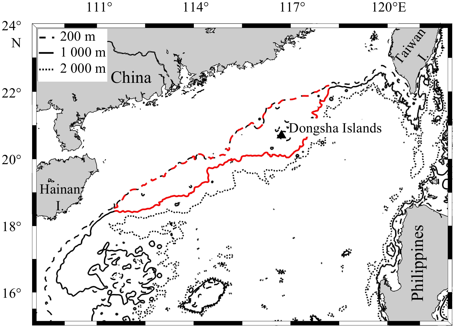
Figure
1.
The topography of the CSR in the northern SCS. The red lines indicate the study area.
| Citation: | Zi Cheng, Meng Zhou, Yisen Zhong, Zhaoru Zhang, Hailong Liu, Lei Zhou. Statistical characteristics of mesoscale eddies on the continental slope in the northern South China Sea[J]. Acta Oceanologica Sinica, 2020, 39(3): 36-44. doi: 10.1007/s13131-019-1530-3

|
The South China Sea (SCS) is the largest marginal sea in the western Pacific Ocean, which spans about 2 000 km and 1 000 km in the meridional and zonal directions, respectively.There are several main channels including Luzon Strait, Kalimantan Strait, Taiwan Strait, Mindoro Strait, and Balabac Strait for water exchanges between the SCS and other ocean. The complexity of the terrain in the SCS with narrow islands shelf in the east, broad continental shelf on the northern and western side, and deep basin in the middle, may play an important role in mean circulation patterns and wave propagation. Considering that the climate in the SCS is dominated by the East Asian monsoon system (Liu et al., 2004), the circulation in the upper layer of the SCS shows strong seasonal signals, with a basin-scale cyclonic gyre in winter, while a smaller anticyclonic gyre in summer (Hu et al., 2000; Su, 2004; Xue et al., 2004).
The enrichment of mesoscale eddy is one of the important features in the northern SCS (Chen et al., 2011; Xiu et al., 2010). In general, the mesoscale eddy is a vortex structure with typical horizontal scales of tens to hundreds of kilometers and time scales on the order of days and months in the ocean, and they tend to contain more energy than ambient mean flow. Meanwhile, nonlinear eddies (do not propagate as Rossby waves) can trap water masses playing an essential role in transporting heat, energy, nutrients and biota (Chelton et al., 2011; Zhai et al., 2008). Mesoscale eddies are regarded as a crucial factor in modulating the climate (Zhang et al., 2014). With the advances in satellite remote sensing and computer computational capacity during last two and three decades, observations and numerical model results have revealed that the northern SCS is an active region for mesoscale eddy generation and interaction (Chen et al., 2011; Hu et al., 2011; Xiu et al., 2010). Previous studies about mesoscale eddies in the SCS have summarized the mechanisms of eddy formation as (1) originating from the interior of the SCS by wind, wind stress curl, flow-topography interaction; (2) originating from the Kuroshio intrusions forming mesoscale eddies in the SCS; and (3) originating from eddies generated in the West Pacific straightly entering the SCS through the Luzon Strait (Zheng et al., 2017).
The Dongsha Islands on the continental slope in the northern SCS is a remarkable atoll where the ambient slope is relatively flat and mesoscale eddies are very vigorous with cross-shelf movement (Luan et al., 2010; Chow et al., 2008; He et al., 2016). Long-lived large cyclonic eddies (CEs) more than several months and over 200 km in diameter were originated almost every year in the south or southwest of the Dongsha Islands (Chow et al., 2008). It is assumed that those eddies are steered by the topography of the Dongsha Islands. Using the model diagnostic calculation, the strong offshore cross-shelf movement appears in the west of the Dongsha Islands (Huang et al., 2017a). To the east of Dongsha Islands, the interaction between baroclinicity and bottom topography leads to deflection of the mid-layer water from isobaths to the deep basin (Wang et al., 2013).
Mesoscale dynamics can also facilitate cross-shelf transport through baroclinicity. In northern California, an anticyclonic eddy off the coast was found to transport plumes of suspended sediments from the continental shelf into the deep ocean (Washburn et al., 1993); and in the southwest of Iberia in winter 2001, eddy-eddy interaction induced the phytoplankton-rich water to form long filaments around the continental margin, which promoted the offshore growth of phytoplankton (Peliz et al., 2004). In the SCS, the enrichment of the mesopelagic fish on the continental slope has high economic value and research prospects (Yuan et al., 2018). In general, it is regarded that the nutrient-rich Zhujiang (Pearl) River plume is trapped by isobaths so that riverine nutrients are limited from the oligotrophic SCS interior (Hu et al., 2000; He et al., 2016). Nevertheless, in the summer of 2015, there was a band of high chlorophyll coastal waters crossed isobaths at the shelf slope into the deep basin area in the west of Dongsha Islands revealed by remote sensing imageries (He et al., 2016). In this band, the Zhujiang River plume water was entrained by the counterclockwise rotation of the CEs. It is also found that the cross-shelf flow is intensified in the intersection of cyclonic-anticyclonic eddy-pair (Chen et al., 2016). Thus, mesoscale eddy process is one of the key mechanisms for water mass exchange onto or off the continental slope.
In this paper, we conduct a statistic study on features of eddy occurrence and propagation in the continental slope region (CSR) of the South China Sea from satellite altimeter data. The CSR is defined as the area enclosed by the 200 m and 1 000 m isobaths in the northern SCS (Fig.1) in which mesoscale eddies are generated and quite active from previous statistical studies (Chen et al., 2011).
The Global Ocean Gridded L4 Sea Surface Heights and Derived Variables Reprocessed product from E.U Copernicus Marine Service Information is used in this analysis (http://marine.copernicus.eu/services-portfolio/access-toproducts/?option=com_csw&view=details&product_id=SEALEVEL_GLO_PHY_L4_REP_OBSERVATIONS_008_047). This product merges all altimeter missions (Jason-3, Sentinel-3A, HY-2A, Saral/AltiKa, Cryosat-2, Jason-2, Jason-1, T/P, ENVISAT, GFO and ERS1/2) and is processed by the SL-TAC multimission altimeter data processing system with respect to a twenty-year mean. Then the data are mapped onto a spatial grid of (1/4)° resolution and archived to daily average from 1993 to present. Only absolute geostrophic velocity and geostrophic velocity anomaly data between 1993 and 2016 are used in this analysis. Due to the potential bias of satellite data in the coastal region, we disregard the the data in shelf regions where the water depth is shallower than 200 m.
Topographic data are essential to reflect the variation of relative position of eddies in the CSR. In this paper, the topographic data (elevation relative to sea level) at half–minute resolution is used from General Bathymetric Chart of the Oceans (GEBCO) 2014 GRID dataset provided by British Oceanographic Data Centre (BODC) (https://www.bodc.ac.uk/data/hosted_data_systems/gebco_gridded_bathymetry_data/).
An eddy detection algorithm employed in this study was developed by Nencioli et al. (2010). This method was based on the geometry of the velocity vectors of the flow field for both detection and tracking:
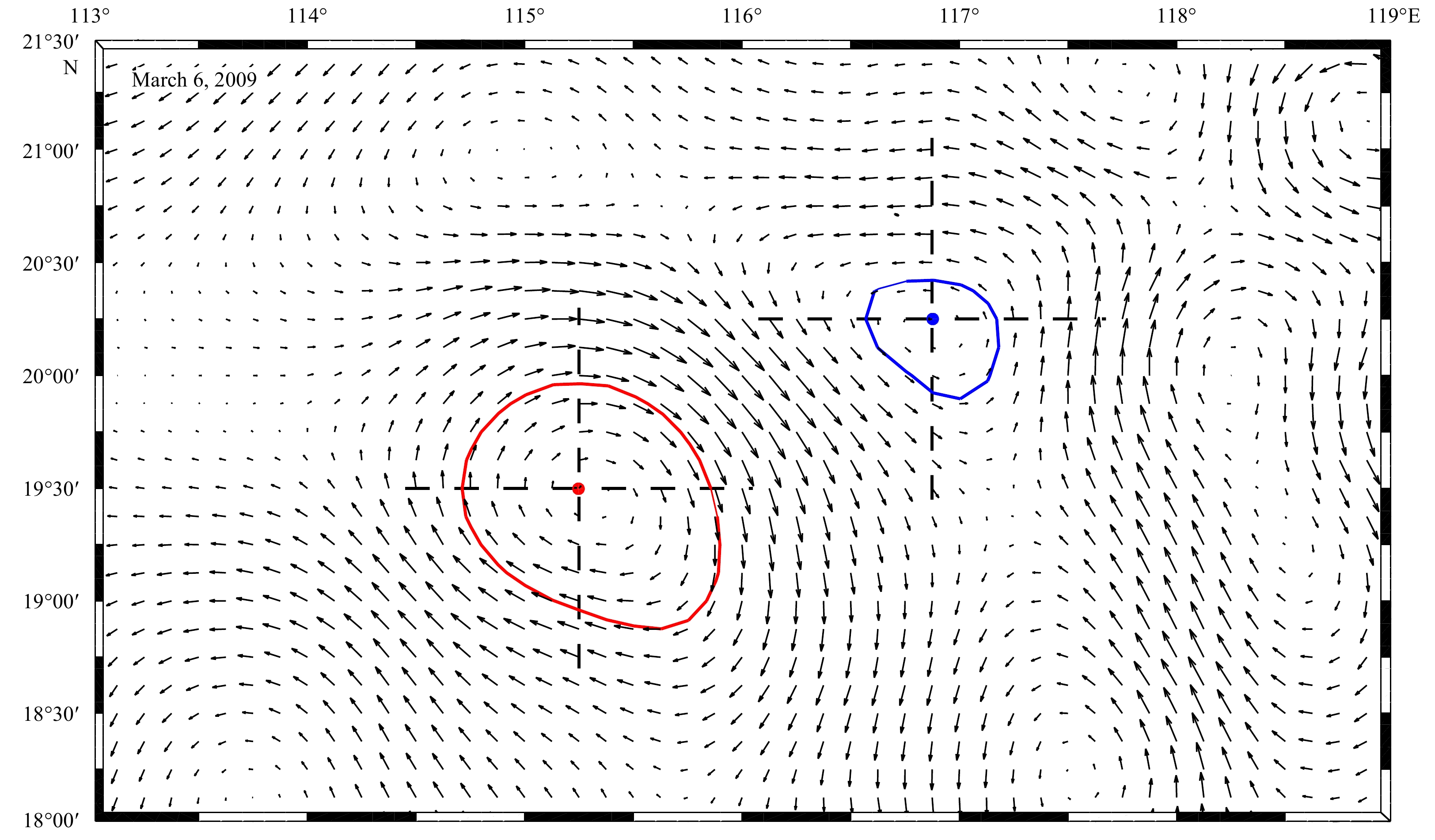
(1) Automatic Eddy Detection Scheme: The algorithm is based on the principle of similarity by which the eddy center must meet specific geometric criteria. Several specific constraints are set to serve as the standards. For example, the minimum velocity should appear at the eddy center, the direction of the velocity vectors on both sides of the center should be opposite, and the magnitude of velocity must increase with the distance from the center. Using the geostrophic current field computed from the satellite altimetry anomaly data in the SCS as an example shown in Fig. 2, if the sign of u component changes from negative to positive when crossing the center from south to north, the rotation is anticyclonic while if the sign of u component changes from positive to negative, the rotation is cyclonic. Because of these criteria on current direction and magnitude changes, this detection method can sometimes underestimate the size of an eddy elucidated by the ACE in Fig 2. Once an eddy center is determined, the boundary is computed by closed contour lines of the streamfunction field.

(2) Eddy Tracking Algorithm: After the eddy is detected at one point, the subsequent work is to determine the next state at consecutive time steps (Δt). The entire process is a so-called eddy tracking. For example, if an eddy center is found at time t, then at time t+Δt, the closest eddy center of the same type (cyclonic/anticyclonic) in the vicinity of the former state will be therefore defined as the continuous state. To ensure the same eddy is tracked, the time step Δt must be significantly smaller than the time scale of eddy deformation such as decay or splitting. Because the movement of vortices is advected by local currents while eddies translate at the speed similar to Rossby waves, both mean current advection and wave propagation within the time interval must be taken into consideration in searching and tracking eddies. An eddy detected will be tracked during the entire period of our study, or till it translates out of the study area. When an eddy cannot be tracked and is missing at time t, for ensuring the accuracy, the detection will be conducted within a larger research area at time t+Δt. If this eddy is still missing, the eddy is considered dissipated.
To ensure the detection and tracking of meso- and large-scale eddies, we only count eddies that live for more than 20 days and have the surface area greater than 10 000 km2 (equivalent eddy scale of 100 km).
The satellite altimetry anomaly data between January 1, 1993 and December 31, 2016 in the SCS-CSR are analyzed by applying the Eulerian Eddy Detection and Tracking Method. There are 147 meso- and large-scale eddies identified inside the CSR, of which 70 and 77 of CEs and ACEs are found, respectively. The distributions, sizes and propagations of these eddies are estimated. It is revealed that eddies in the SCS are affected by Coriolis force, mean currents and topography, and propagate differently in different subdomains (Chen et al., 2011; Zheng et al., 2017).
The spatial distribution of the eddy generation is shown in Fig. 3. Almost all of the eddies in the CSR are generated between 17°N and 22°N in the SCS. There are quite a number of eddies originating from the vicinity of the Dongsha Islands (DS, 19.6°−21.3°N, 115.8°−118.2°E). The other important eddy generation region is located to the southwest of Taiwan (SWT, 19.7°−22°N, 118.3°−120.5°E) away from the margin of the CSR. In the SWT, both CEs and ACEs often coexist revealed by tracking eddy trajectories, and they are often deformed and stretched probably by eddy interaction.

Eddy formation is very common in the vicinity of the DS region as mentioned above, which is consistent with Chow et al. (2008). There are always several eddies existing to the east of this region. Within the study period, a total of 51 eddies (about 35% of all) are counted, 27 of which are CEs and 24 of which are ACEs. In addition, the eddy generation does not show a clear seasonal cycle (Fig. 4). The results from the student t-test indicate that there is no significant discrepancy in eddy formation between the CEs and the ACEs.

Previous studies indicated that the SWT near the Luzon Strait is an essential place for eddy generation in the northern SCS. The ACEs are shed from the Kuroshio Current Loop (KCL) especially in winter, and almost all ACEs shedding from KCL are accompanied by a CE to the northeast (Nan et al., 2011b; Zhang et al., 2017). During the 24-year period of our census, there are 128 eddies generated in the SWT, including 58 CEs and 70 ACEs. Among these eddies, 13 CEs and 26 ACEs can climb up onto the CSR, which account for 22.4% and 37.1% of the total number of CEs and ACEs, respectively. The number of ACE is significantly higher than that of CE, suggesting that ACEs are more capable of moving onto the CSR than CEs. Results shown in Fig. 5 reveals that there is a remarkable seasonal variation in the eddy generation in the SWT. CEs move toward slope mostly in spring, while the ACEs mainly enter the CSR in winter. It is also revealed that the Kuroshio intrudes into the SCS through the Luzon Strait more frequently in winter than in other seasons, and the Kuroshio loop sheds more ACEs in the SWT during winter (Nan et al. 2011a). Thus, these results imply that the stronger Kuroshio intrusion might lead to more ACEs move onto the CSR in winter.

The relative vorticity is typically used to measure the strength of eddies. In this study, we define the vorticity value in the eddy center as the strength of the vortex following Dong (2015). To understand the spatial characteristics of eddy propagation, we average and then normalize the eddy relative vorticity into spatial grid bins (Fig. 6). The spatial patterns of eddy vorticity magnitudes have similar features: large values are found to the east of the Dongsha Islands and relatively small value are found in the middle and west parts of the CSR. This suggests that eddies lose their energy by friction as propagating westwards over the Dongsha Islands.

Moreover, the ACEs are relatively stronger than the CEs in the northeast part of the CSR, which is also mentioned in several previous studies (Fig. 6). For example, studies by both Zhang et al. (2013) and Huang et al. (2017b) indicated that southwest of Taiwan, the CE was weaker than the ACE in an eddy pair. This discrepancy may be caused by differences in the eddy formation mechanism, i.e. CEs are generated from barotropic instability of the northern branch of the KCL, while ACEs are shedding from the KCL and baroclinic instability, and barotropic instability provide energy for its generation and growth (Zhang et al., 2013, 2017).
Eddies will interact dramatically with the topography as moving over continental slope regions (Oey and Zhang, 2004). Many factors such as slope steepness, orientation and even the barotropicity and baroclinicity of water column will significantly influence the vortex motion (Jacob et al., 2002). Regardless of polarity, eddies in the study area have a self-induced westward moving tendency, which can be deduced by β-effect and conventional theories like potential vorticity conservation (Cushman-Roisin et al., 1990). Nevertheless, besides the pure westward motion in the global ocean, eddies also slightly migrate in the meridional direction based on global observed data (Chelton et al., 2007). In terms of the polarity, the CEs and ACEs have poleward and equatorward deflection respectively, which can be adequately explained by potential vorticity conservation as follows: in the northern hemisphere, assuming a β-plane, a relative large eddy could transport water parcels in the meridional direction, and secondary eddies will germinate on the flank. Then the rotation of secondary eddies in turn drive cyclone and anticyclone circulations that move poleward and equatorward respectively (Morrow et al., 2004).
To better understand the eddy propagation properties, the eddy propagation velocities along the trajectories were computed, and then averaged onto 0.25°×0.25° grid bins inside the CSR. Those bins that contain no more than 3 observations were removed for statistical robustness. Most eddies move southwestward along the continental slope. The mean zonal and meridional propagation velocities of the CEs are −5.50 and −6.13 cm/s, and those of ACEs −2.98 and −2.93 cm/s, respectively, which is consistent with earlier studies in the similar region (Chen et al., 2011). If subtracting the speed of mean flow, the mean zonal and meridional velocities of the CEs are changed to −1.16 and 6.50 cm/s, and those of ACEs are changed to 3.92 and −2.99 cm/s, respectively. The CEs and ACEs propagate in opposite meridional directions, with the CEs moving to the shallow region and ACEs to the deep region. This difference can be explained by the conservation of potential vorticity when a CE or ACE loses its energy and rotates more slowly during its movement, the relative vorticity decreases or increases. So that the CE or ACE will move to a shallower or deeper region due to the PV constraint. In general, the ACEs move slightly faster than CEs, which could be properly explained by the effect of the baroclinicity in a two-layer β-plane model proposed by Cushman-Roisin et al. (1990), that is, the discrepancy in the response of water in lower layer to eddies of different polarity leads to the acceleration of ACEs, and deceleration of CEs. There is no straight evidence suggesting any correlation between the propagation speed of Rossby waves and eddies in the CSR. Results based on satellite altimeter data suggested that anticyclonic eddies generated off the northwest coast of Luzon move southwestward along the continental slope are not free long Rossby waves (Yuan et al. 2007). Moreover, compared with the zonal speed of the first baroclinic Rossby wave calculated by Wang et al. (2017), eddies seem to move faster than the Rossby wave on the continental slope.
The mean propagation velocity field of CEs and ACEs in the CSR are elucidated in Fig. 7a and b, respectively. Both CEs and ACEs mainly translate southwestward steered by the topography of the slope. However, the motion directions of the ACEs are more concentrated to some extent, while CEs are inclined to move divergently, which is more intuitively reflected in Fig. 7c and d.

Some eddies tend to move in and out of the CSR several times through their life cycle (not shown). However, these eddies will not stay for long (typically less than 3 days) if they leave the CSR and come back to the slope afterwards. Considering that some eddies only hover on the edge of the CSR or dissipate rapidly as soon as entering the CSR, the statistical standard is redefined as follows: the first day when the eddy appears in the interior of the CSR is set to be the starting point of our statistics, and only those eddies that stay inside the CSR longer than 7 days are considered in our statistical analysis. As a result, 103 eddies meet this standard, including 50 CEs and 53 ACEs. The statistics of the final destinations of those eddies are listed in Table 1. The CEs seem to have higher chance to leave the CSR because the number of CEs dissipated in the CSR is relatively low compared with that of ACEs. However, a number of those CEs just wander between the margin of the CSR and the deep basin (1 000−3 000 m).
| Polarity | Dissipating in the continental slope | Leaving the continental slope | ||
| Basinward (>2 000 m) | Shelfward (<200 m) | Others | ||
| CE | 26 (52%) | 3 | 4 | 17 |
| ACE | 33 (62%) | 5 | 6 | 9 |
 DownLoad:
CSV
DownLoad:
CSV
The relationship between water depths of an eddy center and its life span by averaging all eddies of the same polarity is shown in Fig. 8a. Both ACEs and CEs cross isobaths onto shallow depth in the similar pattern for the first 6 days, and then move in significantly different patterns afterward. The depth variations of CEs are much larger than that of ACEs between 6 and 30 days when moving into the CSR These non-overlapping of confidence intervals indicate the significant difference in motion between these two types of eddies. Further, the depth variations of individual eddies indicate the similarity and differences between CEs and ACEs (Figs. 8b and c), that is, in the initial stage of 6 days, CEs generally spread across the isobaths in the similar range, between 6 and 30 days, the center depths of ACEs spread in a significant larger range than that of CEs, and in late stage longer than 30 days, more ACEs are inclined to move to the deeper basin while CEs continue to propagate along the edge of the CSR.

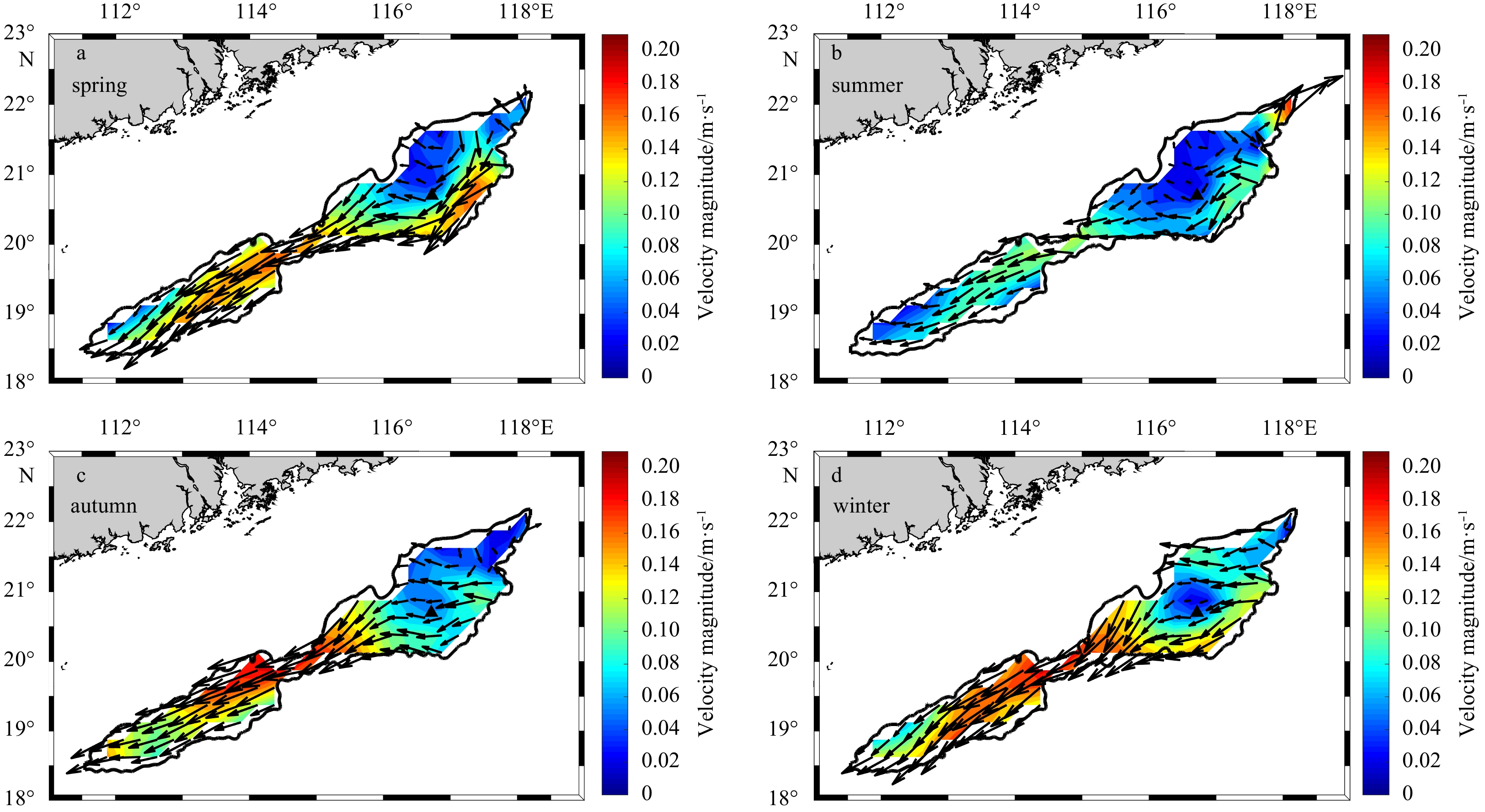
The seasonal forcing in the SCS is dominated by seasonal East Asian monsoon, which reverses the direction of the upper-layer circulation over the entire basin between seasons (Hu et al., 2000). In the CSR, the seasonal variation is reflected in the change in the strength of the along-slope current, i.e., the current is stronger in winter and weaker in summer (Fig. 9). During all seasons, the flow accelerates within the narrow slope corridor between 114.5°−115.5°E, which might be explained by the “venturi effect”-the expediting of the fluid when it flows through a constricted section of the terrain. Besides, in winter, the geostrophic currents in the CSR tend to bifurcate into two branches, one flowing to the region west of the Dongsha Islands and the other going down the slope, which could facilitate the cross-shelf transport in that area.

To better understand the impact of mean flow on the eddy propagation in the CSR, we plot the eddy trajectories in each season (Fig. 10). Consistent with results shown in Fig. 9, the eddy propagation is in agreement with the along-slope current to a large degree. For example, in winter and autumn, eddies are propagating with the mean flow along the slope. In summer, eddies move randomly, and the trajectories diverge because of weaker wind and mean flows. More eddies tend to cross the mean flow and the isobaths so that cross-shelf transport is likely to take place in this season (He et al., 2016). In winter, eddies are prone to leave the CSR in the ambient region west of the Dongsha Islands in agreement with the downward slope current. Among those eddies, the ACEs are dominant both in quantity and propagation distance, and some of them can even reach south of 16°N.

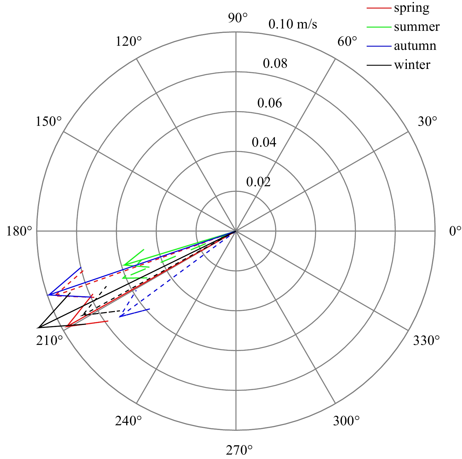
The comparison in the direction and magnitude between the seasonal geostrophic current and eddy propagation velocities are shown in Fig. 11 and Table 2. The results show a good correlation between these two velocities in all seasons. In autumn and winter, geostrophic speed is slightly larger than the eddy propagation speed, and the direction of these two velocities almost overlap in winter. However, in summer, eddies propagate without strong constraints due to weak mean currents and even move a little faster than the ambient mean flow. In conclusion, there are no statistical differences between mean current and eddy propagation velocities, and the seasonal variations of the eddy behavior is probably owing to the seasonal change of the along-slope current.

| Season | Geostrophic velocity(GV) | Eddy propagation velocity(EPV) | Speed ratio (EPV/GV) | Angle difference/(°) (EPV-GV) | |||
| Velocity magnitude/m·s–1 | Angel/(°) | Velocity magnitude/m·s–1 | Angel/(°) | ||||
| Spring | 0.098 | 209.46 | 0.096 | 201.80 | 0.99 | –9.785 | |
| Summer | 0.059 | 196.95 | 0.062 | 201.45 | 1.05 | 5.709 | |
| Autumn | 0.099 | 198.86 | 0.070 | 216.40 | 0.73 | 17.533 | |
| Winter | 0.110 | 206.11 | 0.083 | 210.97 | 0.80 | 2.684 | |
DownLoad:
CSV
The eddy propagation properties on the continental slope region in the northern SCS are analyzed based on 24-year satellite altimeter data by employing a Eulerian eddy detection and tracking method. The broad continental slope in the northern SCS is an active region for the eddy generation and propagation (Chen et al., 2011; Xiu et al., 2010). In this study period, 147 large eddies including 70 CEs and 77 ACEs are detected in the CSR, 103 of which including 50 CEs and 53 ACEs remain inside the CSR for more than 6 days. There are two important source regions for the eddy formation, the surrounding region of the Dongsha Islands where eddies are generated without a noticeable seasonal cycle, and the Southwest region of Taiwan where ACEs are generated in the majority primarily in winter. After these eddies are generated in the CSR, eddies mainly propagate along the slope under the constraint of bathymetry and tend to weaken during their westward movement. During life spans of these eddies, the ACEs move slightly faster than CEs in the zonal direction attributed to the baroclinicity of the water column; in the CSR the CEs are more inclined to cross the isobaths than the ACEs; after departure from the CSR, most CEs are confined by the 3 000-m isobath while several long-lived ACEs penetrate to the deep basin. The interactions between eddies and mean currents in the CSR have a notable seasonal pattern. In summer, due to the weak background currents, eddies diverge their path from the mean flow axis, and the onshore eddy movement mainly takes place in this season; and in autumn and winter, eddies are carried by the mean flow, and the strong constraint of the mean flow limits the cross-shelf eddy movement. The results also reveal that downslope tendency of currents on the west side of Dongsha Islands while eddies leave the CSR around the same site in a cluster.
The altimeter data is provided by E.U. Copernicus Marine Service Information. We also appreciate the eddy detection method provided by Changming Dong from Nanjing University of Information Science & Technology.
| [1] |
Chelton D B, Schlax M G, Samelson R M, et al. 2007. Global observations of large oceanic eddies. Geophysical Research Letters, 34(15): L15606
|
| [2] |
Chelton D B, Schlax M G, Samelson R M. 2011. Global observations of nonlinear mesoscale eddies. Progress in Oceanography, 91(2): 167–216. doi: 10.1016/j.pocean.2011.01.002
|
| [3] |
Chen Gengxin, Hou Yijun, Chu Xiaoqing. 2011. Mesoscale eddies in the South China Sea: Mean properties, spatiotemporal variability, and impact on thermohaline structure. Journal of Geophysical Research, 116(C6): C06018
|
| [4] |
Chen Zhongwei, Yang Chenghao, Xu Dongfeng, et al. 2016. Observed hydrographical features and circulation with influences of cyclonic-anticyclonic eddy-pair in the northern slope of the South China Sea during June 2015. Journal of Marine Sciences (in Chinese), 34(4): 10–19
|
| [5] |
Chow C H, Hu J H, Centurioni L R, et al. 2008. Mesoscale Dongsha Cyclonic Eddy in the northern South China Sea by drifter and satellite observations. Journal of Geophysical Research: Oceans, 113(C4): C04018
|
| [6] |
Cushman-Roisin B, Tang B, Chassignet E P. 1990. Westward motion of mesoscale eddies. Journal of Physical Oceanography, 20(5): 758–768. doi: 10.1175/1520-0485(1990)020<0758:WMOME>2.0.CO;2
|
| [7] |
Dong Changming. 2015. Oceanic Eddy Detection and Analysis (in Chinese). Beijing: Science Press
|
| [8] |
He Xianqiang, Xu Dongfeng, Bai Yan, et al. 2016. Eddy-entrained Pearl River plume into the oligotrophic basin of the South China Sea. Continental Shelf Research, 124: 117–124. doi: 10.1016/j.csr.2016.06.003
|
| [9] |
Hu Jianyu, Kawamura H, Hong Huasheng, et al. 2000. A review on the currents in the South China Sea: Seasonal Circulation, South China Sea warm current and Kuroshio intrusion. Journal of Oceanography, 56(6): 607–624. doi: 10.1023/A:1011117531252
|
| [10] |
Hu Jianyu, Gan Jianping, Sun Zhenyu, et al. 2011. Observed three-dimensional structure of a cold eddy in the southwestern South China Sea. Journal of Geophysical Research: Oceans, 116(C5): C05016
|
| [11] |
Huang Xiaodong, Zhang Zhiwei, Zhang Xiaojiang. 2017a. Impacts of a mesoscale eddy pair on internal solitary waves in the Northern South China Sea revealed by mooring array observations. Journal of Physical Oceanography, 47(7): 1539–1554. doi: 10.1175/JPO-D-16-0111.1
|
| [12] |
Huang Xiaorong, Wang Qiang, Zhou Weidong. 2017b. Model diagnostic analysis of cross-shelf flow in the northern South China Sea. Chinese Science Bulletin, 62(10): 1059–1070. doi: 10.1360/N972016-00570
|
| [13] |
Jacob J P, Chassignet E P, Dewar W K. 2002. Influence of topography on the propagation of isolated eddies. Journal of Physical Oceanography, 32(10): 2848–2869. doi: 10.1175/1520-0485(2002)032<2848:IOTOTP>2.0.CO;2
|
| [14] |
Liu Qinyu, Jiang Xia, Xie Shangping, et al. 2004. A gap in the Indo-Pacific warm pool over the South China Sea in boreal winter: Seasonal development and interannual variability. Journal of Geophysical Research: Oceans, 109(C7): C07012
|
| [15] |
Luan Xiwu, Zhang Liang, Yue Baojing. 2010. Influence on gas hydrates formation produced by volcanic activity on northern South China Sea slope. Geoscience (in Chinese), 24(3): 424–432
|
| [16] |
Morrow R, Birol F, Griffin D, et al. 2004. Divergent pathways of cyclonic and anti-cyclonic ocean eddies. Geophysical Research Letters, 31(24): L24311. doi: 10.1029/2004GL020974
|
| [17] |
Nan Feng, Xue Huijie, Xiu Peng, et al. 2011a. Oceanic eddy formation and propagation southwest of Taiwan. Journal of Geophysical Research: Oceans, 116(C12): C12045. doi: 10.1029/2011JC007386
|
| [18] |
Nan Feng, Xue Huijie, Chai Fei, et al. 2011b. Identification of different types of Kuroshio intrusion into the South China Sea. Ocean Dynamics, 61(9): 1291–1304. doi: 10.1007/s10236-011-0426-3
|
| [19] |
Nencioli F, Dong Changming, Dickey T, et al. 2010. A vector geometry-based eddy detection algorithm and its application to a high-resolution numerical model product and high-frequency radar surface velocities in the Southern California Bight. Journal of Atmospheric and Oceanic Technology, 27(3): 564–579. doi: 10.1175/2009JTECHO725.1
|
| [20] |
Oey L Y, Zhang H C. 2004. The generation of subsurface cyclones and jets through eddy-slope interaction. Continental Shelf Research, 24(18): 2109–2131. doi: 10.1016/j.csr.2004.07.007
|
| [21] |
Peliz A, Santos M P, Oliveira P B, et al. 2004. Extreme cross-shelf transport induced by eddy interactions southwest of Iberia in winter 2001. Geophysical Research Letters, 31(8): L08301
|
| [22] |
Su Jilan. 2004. Overview of the South China Sea circulation and its influence on the coastal physical oceanography outside the Pearl River Estuary. Continental Shelf Research, 24(16): 1745–1760. doi: 10.1016/j.csr.2004.06.005
|
| [23] |
Wang Dongxiao, Wang Qiang, Zhou Weidong, et al. 2013. An analysis of the current deflection around Dongsha Islands in the northern South China Sea. Journal of Geophysical Research: Oceans, 118(1): 490–501. doi: 10.1029/2012JC008429
|
| [24] |
Wang Dingqi, Fang Guohong, Qiu Ting. 2017. The characteristics of eddies shedding from Kuroshio in the Luzon Strait. Oceanologia et Limnologia Sinica (in Chinese), 48(4): 672–681
|
| [25] |
Washburn L, Swenson M S, Largier J L, et al. 1993. Cross-shelf sediment transport by an anticyclonic eddy off northern California. Science, 261(5128): 1560–1564. doi: 10.1126/science.261.5128.1560
|
| [26] |
Xiu Peng, Chai Fei, Shi Lei, et al. 2010. A census of eddy activities in the South China Sea during 1993–2007. Journal of Geophysical Research: Oceans, 115(C3): C03012
|
| [27] |
Xue Huijie, Chai Fei, Pettigrew N, et al. 2004. Kuroshio intrusion and the circulation in the South China Sea. Journal of Geophysical Research: Oceans, 109(C2): C02017
|
| [28] |
Yuan Dongliang, Han Weiqing, Hu Dunxin. 2007. Anti-cyclonic eddies northwest of Luzon in summer-fall observed by satellite altimeters. Geophysical Research Letters, 34(13): L13610
|
| [29] |
Yuan Meng, Chen Zuozhi, Zhang Jun, et al. 2018. Community structure of mesopelagic fish species in northern slope of South China Sea. South China Fisheries Science (in Chinese), 14(1): 85–91
|
| [30] |
Zhai Xiaoming, Greatbatch R J, Kohlmann J D. 2008. On the seasonal variability of eddy kinetic energy in the Gulf Stream region. Geophysical Research Letters, 35(24): L24609. doi: 10.1029/2008GL036412
|
| [31] |
Zhang Zhiwei, Zhao Wei, Tian Jiwei, et al. 2013. A mesoscale eddy pair southwest of Taiwan and its influence on deep circulation. Journal of Geophysical Research: Oceans, 118(12): 6479–6494. doi: 10.1002/2013JC008994
|
| [32] |
Zhang Zhengguang, Wang Wei, Qiu Bo. 2014. Oceanic mass transport by mesoscale eddies. Science, 345(6194): 318–322. doi: 10.1126/science.1249770
|
| [33] |
Zhang Zhiwei, Zhao Wei, Qiu Bo, et al. 2017. Anticyclonic eddy sheddings from kuroshio loop and the accompanying cyclonic eddy in the northeastern South China Sea. Journal of Physical Oceanography, 47(6): 1243–1259. doi: 10.1175/JPO-D-16-0185.1
|
| [34] |
Zheng Quanan, Xie Lingling, Zheng Zhiwen, et al. 2017. Progress in research of mesoscale eddies in the South China Sea. Advances in Marine Science (in Chinese), 35(2): 131–158
|
| 1. | Wenjing Zhang, Chen Zhang, Shan Zheng, et al. Distribution of picophytoplankton in the northern slope of the South China Sea under environmental variation induced by a warm eddy. Marine Pollution Bulletin, 2023, 194: 115429. doi:10.1016/j.marpolbul.2023.115429 | |
| 2. | Xiayan Lin, Guixi Wang, Guoqing Han, et al. Cross-Slope Transport by a Mesoscale Anticyclone in the Northern South China Sea. Journal of Marine Science and Engineering, 2023, 11(2): 305. doi:10.3390/jmse11020305 | |
| 3. | Ye Lu, Yu Zhang, Jiahua Wang, et al. Dynamics in Bacterial Community Affected by Mesoscale Eddies in the Northern Slope of the South China Sea. Microbial Ecology, 2022, 83(4): 823. doi:10.1007/s00248-021-01816-6 | |
| 4. | Chao Yan, Jing Feng, Ping-Lv Yang, et al. A new algorithm for reconstructing the three-dimensional flow field of the oceanic mesoscale eddy*. Chinese Physics B, 2021, 30(12): 120204. doi:10.1088/1674-1056/ac29af |

Figures(11) / Tables(2)

Supported by:
Beijing Renhe Information Technology Co. Ltd

Zi Cheng, Meng Zhou, Yisen Zhong, Zhaoru Zhang, Hailong Liu, Lei Zhou. Statistical characteristics of mesoscale eddies on the continental slope in the northern South China Sea[J]. Acta Oceanologica Sinica, 2020, 39(3): 36-44. doi: 10.1007/s13131-019-1530-3

| Polarity | Dissipating in the continental slope | Leaving the continental slope | ||
| Basinward (>2 000 m) | Shelfward (<200 m) | Others | ||
| CE | 26 (52%) | 3 | 4 | 17 |
| ACE | 33 (62%) | 5 | 6 | 9 |
DownLoad:
CSV
| Season | Geostrophic velocity(GV) | Eddy propagation velocity(EPV) | Speed ratio (EPV/GV) | Angle difference/(°) (EPV-GV) | |||
| Velocity magnitude/m·s–1 | Angel/(°) | Velocity magnitude/m·s–1 | Angel/(°) | ||||
| Spring | 0.098 | 209.46 | 0.096 | 201.80 | 0.99 | –9.785 | |
| Summer | 0.059 | 196.95 | 0.062 | 201.45 | 1.05 | 5.709 | |
| Autumn | 0.099 | 198.86 | 0.070 | 216.40 | 0.73 | 17.533 | |
| Winter | 0.110 | 206.11 | 0.083 | 210.97 | 0.80 | 2.684 | |
DownLoad:
CSV
| Polarity | Dissipating in the continental slope | Leaving the continental slope | ||
| Basinward (>2 000 m) | Shelfward (<200 m) | Others | ||
| CE | 26 (52%) | 3 | 4 | 17 |
| ACE | 33 (62%) | 5 | 6 | 9 |
| Season | Geostrophic velocity(GV) | Eddy propagation velocity(EPV) | Speed ratio (EPV/GV) | Angle difference/(°) (EPV-GV) | |||
| Velocity magnitude/m·s–1 | Angel/(°) | Velocity magnitude/m·s–1 | Angel/(°) | ||||
| Spring | 0.098 | 209.46 | 0.096 | 201.80 | 0.99 | –9.785 | |
| Summer | 0.059 | 196.95 | 0.062 | 201.45 | 1.05 | 5.709 | |
| Autumn | 0.099 | 198.86 | 0.070 | 216.40 | 0.73 | 17.533 | |
| Winter | 0.110 | 206.11 | 0.083 | 210.97 | 0.80 | 2.684 | |
 DownLoad:

 DownLoad: