Mediterranean Sea level trends from long-period tide gauge time series

1. Introduction

Originally, tide gauges were deployed for navigation and tidal prediction. Their scope has expanded considerably from coastal engineering and coastal management to climate change, of which the sea level is an essential parameter. There are several long sea level records discussed in the literature which are historically important. Van Veen (1954) was the first to take an interest in historical measurements of sea level by constructing the series of annual mean observations for Amsterdam for the period of 1700–1925. To study the long-term variations of tidal components, Cartwright (1972a, b) also studied this type of measure. In the late 1980s, Hannah (1988, 1990) reconstructed tidal observations series for several ports in New Zealand. In 1988, historical annual mean values for Stockholm are published by Ekman (1988). In the late 1990s, new multi-scale series were reconstructed with Liverpool (Woodworth, 1999a, b) and Kronstadt (Bogdanov et al., 2000). Although the tide gauge time series are constructed to be continuous and are often used to study long-term variations in currents and the volume of water in the oceans, which can be affected by changes in temperature, salinity, and the balance of fresh water flux and evaporation, other geophysical signals are also present in these data: Glacial Isostatic Adjustment (GIA), earthquakes, ground water extraction and sedimentation.

Currently, the PSMSL, established in 1933, is responsible for the collection, publication, analysis and interpretation of sea level data from the global network of tide gauges. The most familiar application based on PSMSL’s data is the global and the regional sea level rise and variability. The PSMSL data set is the main source of information on long term changes in the global sea level during the last two centuries. Data have been employed intensively in studies such as those of Intergovernmental Panel on Climate Change (IPCC). The latest IPCC report, published in 2013, finds that it is very likely that the mean rate of global averaged sea level rise was 1.7 mm/a between 1901 and 2010, 2.0 mm/a between 1971 and 2010 and 3.2 mm/a between 1993 and 2010 (IPCC, 2013).

This report indicates also the Mediterranean, being a land-locked sea, as one of the most vulnerable regions in the world to the impact of climate change, expecting an increase in average surface temperatures (to the base period of 1980–2000) in the range of 2.2 and 5.1°C for the period of 2080–2100. This further indicates an increasing heat content of this basin which can directly translates into an increase in the mean sea level by thermal expansion. A possible impact of the sea-level rise is further enhanced in the Mediterranean Sea by the presence, particularly along the coasts, of densely populated areas and a high-value economical activity. The problem of the long term sea level analysis in the Mediterranean Sea has been tackled in a number of studies based on tide gauges observations. The analysis of the longest tide gauges series in the the Mediterranean Sea coasts indicate a rate of the sea level rise, for the 20th century, of 1.1–1.3 mm/a (Tsimplis and Baker, 2000). During the period of 1960–1990, an increase in the average atmospheric pressure over the basin caused negative sea level trends. During the same period, the sea level was rising in the Atlantic stations but with a lower rate than before 1960 (Tsimplis and Baker, 2000; Tsimplis and Josey, 2001). Whereas the sea level appears to have increased globally from the 1980s (Holgate and Woodworth, 2004; Holgate, 2007), a fast sea level rise was observed in the Mediterranean only in late 1990s (Cazenave et al., 2001; Fenoglio-Marc, 2001).

Regionally and in the western Mediterranean Sea, Marseille and Genova tide gauges are two of the few European tide gauge records in the Mediterranean Sea spanning more than one hundred years. The estimated rate of the sea level change is of 1.2 mm/a in Marseille and in the nearby Genova tide gauge for a period starting in 1885 (Marcos and Tsimplis, 2008). In the semi-enclosed basin of Adriatic Sea, a trend of 1.25 mm/a was highlighted for the time period between 1872 and 2012 (Galassi and Spada, 2014). Some earlier studies of the southern Levantine sub-basin used tide-gauge data. At Alexandria, the longest available time series in the region, the mean sea level indicated two regimes. Before the Aswan High Dam was built, Alexandrian sea levels display a strong significant rising trend of 5 mm/a from 1944 to 1963 (Shaltout et al., 2015). This strong trend is probably attributable to sedimentation from the Nile that caused sinking of the land surface. After the building of the dam, the sea-level trend has weakened to approximately 0.2 mm/a from 1964 to 2006. Other studies of the Alexandrian mean sea-level displayed a positive trend of 2 mm/a from 1944 to 1989 (Frihy, 1992), 1.6 mm/a from 1944 to 2001 (Frihy, 2003), and 3 mm/a from 1974 to 2006 (Said et al., 2012).

Despite the above general statements which are derived on the basis of the longest tide gauges available, there are several other tide gauges in the Mediterranean Sea providing information regarding local sea level variability. This study reports the long-term relative Mediterranean sea-level trends from tide gauge measurements by a different statistical approach instead of a linear regression in time, which is a widely used method by scientists to estimate trends. To this end, the series of monthly values of sea level were analyzed for monotonous increasing or decreasing trends with the non-parametric Mann-Kendall test (Mann, 1945; Kendall, 1975; Hirsch et al., 1982) and Sen’s method for slope estimates (Sen, 1968; Hirsch et al., 1982). One advantage of the Mann-Kendall test is that data do not need any particular distribution. The second advantage of the test is its low sensitivity to abrupt breaks (change-points) in the time series (Tabari et al., 2011). Sen’s method uses a linear model to estimate the slope of the trend (change per unit time) and the variance of the residuals should be constant in time (Salmi et al., 2002).

The rest of the paper is organized as follows. Section 2 describes the datasets used in this study. The Mann-Kendall test used for trend detection and the Sen’s slope approach used to estimate the magnitude of trends are briefly explained in Section 3. The empirical results of the trends identification and the sea level rise estimations in the Mediterranean Sea are addressed in Section 4. Section 5 concludes.

2. The data

The study of the trend does not necessarily require direct manipulation of hourly tide gauge data. Indeed, the mechanism for calculating the average hourly data for one month or one year filter the fluctuations of short period observed in tide gauge records, that are of irregular nature (waves of storm, tidal wave…) or periodical (diurnal, tidal waves, tides…). The time series of monthly or annual averages are, consequently suitable, under investigation of the sea level long-term variations. However, the trend estimation raises a first question over the minimal length of the time series. Some authors limit their study to more or less arbitrary observation periods. For example, Gutenberg (1941) considers in his study only the stations which, at the time, had at least 15 years of measurements. Gornitz et al. (1982) choose the tide gauges of more than 20 years of records, whereas Barnett (1984) selected only stations that have over 30 years of data. More recently, Trupin and Wahr (1990) fixed the low limit at 40 years; Peltier and Tushingham (1991) chooses the 50 years values, but Douglas (1991) choose the strongest constraint with a minimum duration of 60 years of records. A consensual value seems to emerge around 40 to 50 years; this duration would represent a reasonable climatic basis to estimate the current eustatic variations and to filter the cyclic and irregular contributions of tide gauges signal (Wöppelmann, 1997). Other criteria are, also sometimes, taken into account in the choice of the tide gauges data, for example, the noise of the data, or the geographical location of the instrument.

In this context, we chose within the framework of this study to analyze the available monthly averages sea level series with more than 50 years of measurements: Tarifa (Spain), Algeciras (Spain), Malaga (Spain), Marseille (France), Genova (Italy), Venezia (Punta Della Salute) (Italy), Trieste (Italy), Rovinj (Croatia), Bakar (Croatia), Split Rt Marjana (Croatia), Split–Gradska Luka (Croatia), Dubrovnik (Croatia), Alexandria (Egypt) and Ceuta (Spain).

The corresponding monthly tidal heights series are obtained from the Internet site of the PSMSL^①. These data are the “RLR” (Revised Local Refers) category, in other words, those which underwent several test, controls and processing aiming to check the continuity and the local stability of the tide gauge reference (Holgate et al., 2013; PSMSL, 2018). In order to avoid negative numbers in the resulting RLR monthly and annual mean values, the RLR datum for each station is defined to be approximately 7 000 mm below mean sea level. However, corrections for the vertical movement for the reference, e.g. due to GIA which on a long-term temporal scale can have a significant impact, are not applied, because this requires a careful estimation of these movements usually involving a geodynamic model (PSMSL, 2018).

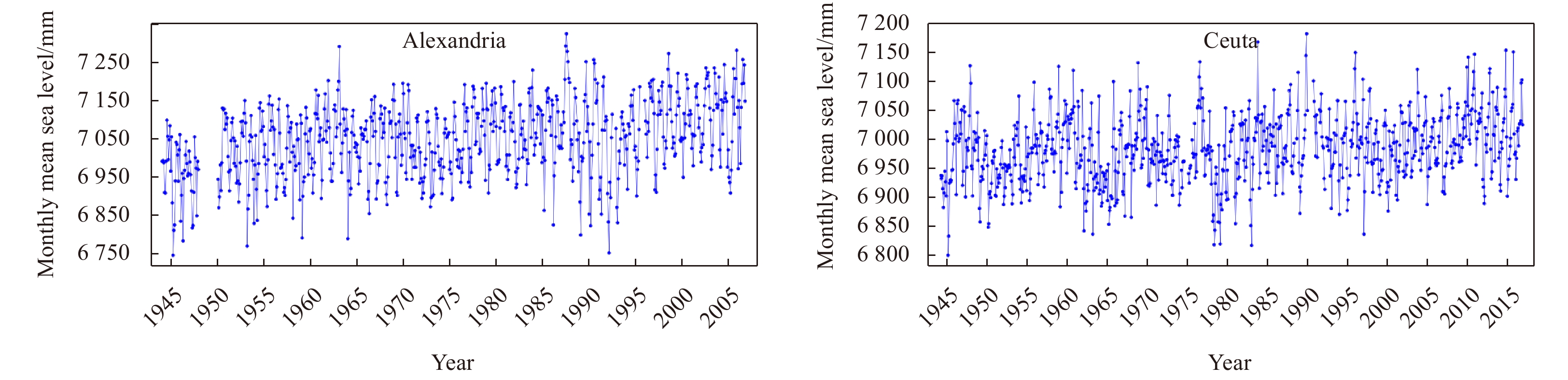
Figure 1 represents the used tidal heights series (in mm). Following Marseille station documentation^②, there were possible faulty data over the period 1951–1952. Also, the values for 2005/06 are flagged suspect. Following Rovinj station documentation^③, the values for February-March 1958 and November-December 1960 seem low compared to Trieste. The station of Bakar is subject to anomalous values for January-March 1951, caused by float wire problems^④.

Figure  1.  Monthly mean sea level (in mm). From top to bottom and from left to right: Tarifa (Spain), Algeciras (Spain), Malaga (Spain), Marseille (France), Genova (Italy), Venezia (Punta Della Salute) (Italy), Trieste (Italy), Rovinj (Croatia), Bakar (Croatia), Split Rt Marjana (Croatia), Split-Gradska Luka (Croatia), Dubrovnik (Croatia), Alexandria (Egypt) and Ceuta (Spain).

DownLoad: Full-Size Img PowerPoint

The descriptive statistics of tide gauge data for the 14 stations selected are given in Table 1. The slope for the linear trend and its standard deviation of the residual variability are estimated using the classical least squares method that finds the line of best fit for a dataset. The most common application of this method aims to create a straight line that minimizes the sum of the squares of the residuals resulting from differences in the observed value and the value anticipated based on the model.

Table  1.  Descriptive statistics of used tide gauge data.

PSMSL station code	Station	Latitude/ (°)	Longitude/ (°)	Data range	Obs.	Obs. with missing data	Obs. without missing data	Slope/ mm·a–1	Standard deviation/ mm·a–1
220/021	Tarifa	36.008 600	–5.602 600	1943–2016	880	50	830	1.14	0.12
220/011	Algeciras	36.116 669	–5.433 333	1943–2002	711	127	584	0.37	0.13
220/031	Malaga	36.712 700	–4.415 460	1944–2013	840	149	691	0.78	0.14
230/051	Marseille	43.278 801	5.353 860	1885–2016	1 583	48	1 535	1.31	0.05
250/011	Genova	44.400 000	8.900 000	1884–1997	1 368	297	1 071	1.19	0.06
270/054	Venezia (Punta Della Salute)	45.433 333	12.333 333	1909–2000	1 104	65	1 039	2.44	0.10
270/061	Trieste	45.647 361	13.758 472	1875–2016	1 704	230	1 474	1.32	0.06
280/006	Rovinj	45.083 300	13.628 300	1955–2014	714	3	711	0.85	0.18
280/011	Bakar	45.300 000	14.533 333	1930–2013	1 008	132	876	1.10	0.13
280/021	Split Rt Marjana	43.508 333	16.391 667	1952–2011	716	8	708	–0.01	0.18
280/031	Split–Gradska Luka	43.506 700	16.441 700	1954–2014	730	0	730	1.06	0.17
280/081	Dubrovnik	42.658 300	18.063 300	1956–2014	708	7	701	1.56	0.17
330/071	Alexandria	31.216 667	29.916 667	1944–2006	755	33	722	1.77	0.17
340/001	Ceuta	35.892 400	–5.315 890	1944–2016	874	28	846	0.68	0.09

 | Show Table

DownLoad: CSV

As show in Table 1, the series show a significant positive trend with the exception of Split Rt Marjana series that exhibits a priori a negative slope of –0.01 mm/a. However the reliability of this negative slope is rather suspicious in view of its strong error margin (±0.18 mm/a). This is why we must take into account the problem of the presence or not of significant monotonic trends in the time series before any slope estimation of the trend.

3. Methods

3.1 Mann-Kendall test

The Mann-Kendall trend test is a nonparametric test used to identify a trend in a series, even if there is a seasonal component in the series. This test is the result of the development of the nonparametric trend test first proposed by Mann (1945). This test was further studied by Kendall (1975) and improved by Hirsch et al. (1982) who allowed taking into account seasonality. The Mann-Kendall test is commonly employed to detect monotonic trends in series of environmental data, climate data or hydrological data. The null hypothesis, H₀, is that data come from a population within dependent realizations and are identically distributed. The alternative hypothesis, H_A, is that data follow a monotonic trend. The Mann-Kendall test statistic is calculated according to:

with:

The variance of S is:

where, number of the tied groups in the data set and t_j: number of data points in the jth tied group. The statistic S is approximately normal distributed provided that the following Z-transformation is employed:

A positive value of Z indicates an increasing trend and a negative value indicates a decreasing trend, and the Kendall's τ is given by:

The seasonal Mann-Kendall statistic for the gth season is calculated as:

According to Hirsch et al. (1982), the seasonal Mann-Kendall statistic, $\hat S$, for the entire series is calculated according to:

For further information, the reader is referred to Hipel and McLeod (1994) and Hirsch et al. (1982).

3.2 Sen's slope

This test computes both the slope (i.e. linear rate of change) and intercept according to Sen's method. First, a set of linear slopes is calculated as follows (Sen, 1968):

for 1≤i<j≤n, where d is the slope, X denotes the variable, n is the number of data, and i, j are indices. Sen's slope is then calculated as the median from all slopes: b=Median d_k. The intercepts are computed for each time step t as given by:

and the corresponding intercept is as well the median of all intercepts.

According to Hirsch et al. (1982) the seasonal Sen's slope is calculated using the following formula:

For each (x_ij, x_ik) pair i=1,2,…,m, where 1≤k≤j≤n_i and n_i is the number of known values in the ith season. The seasonal slope estimator is the median of the d_ijk values.

4. Empirical results and discussion

In this section, the calculations were made under the R Programming environment using the software package “trend” of Pohlert (2016) from the German Federal Institute of Hydrology (BfG). This package presents a collection of non-parametric methods for the time series analysis. It provides the Mann-Kendall Trend Test, the seasonal Mann-Kendall test and (seasonal) Sen’s slope. Using these methods, we analyze separately each sea level time series to determine its long term trend.

4.1 Trend detection

The two tests are applied: the classical Mann-Kendall test to test if there is a significant trend in the sea level time series; the seasonal Mann-Kendall test that takes into account the seasonality in the time series (here 12 months).

Table 2 gives a summary of the obtained results of the first test for the 14 sea level time series. The null hypothesis H₀ for the Mann-Kendall test is that there is no trend in the series. The three alternative hypotheses H_a are that there is a negative, non-null, or positive trend. It can be seen, from Table 2, that with the exception of the Split Rt Marjana series (p=0.263), the obtained p values for the remaining data are lower than the fixed significance level (α=0.05). One should reject the null hypothesis H₀, and accept the alternative hypothesis H_a. We can conclude that there are significant positive trends in our sea level series (S>0).

Table  2.  Man-Kendall trend test

PSMSL station code	Station	Data range	Mann-Kendall statistic S	Var S	p value	Risk to reject the null hypothesis H0 while it is true/%
220/021	Tarifa	1943–2016	77 957.000	63 644 155.667	<0.000 1	<0.01
220/011	Algeciras	1943–2002	11 249.000	22 185 786.333	0.017	1.69
220/031	Malaga	1944–2013	39 630.000	36 737 888.667	<0.000 1	<0.01
230/051	Marseille	1885–2016	503 942.000	402 249 772.000	<0.000 1	<0.01
250/011	Genova	1884–1997	211 644.000	1 366 844 12.667	<0.000 1	<0.01
270/054	Venezia (Punta Della Salute)	1909–2000	230 566.000	124 801 981.333	<0.000 1	<0.01
270/061	Trieste	1875–2016	407 832.000	356 190 664.667	<0.000 1	<0.01
280/006	Rovinj	1955–2014	33 495.000	40 018 652.333	<0.000 1	<0.01
280/011	Bakar	1930–2013	80 595.000	74 816 433.000	<0.000 1	<0.01
280/021	Split Rt Marjana	1952–2011	7 043.000	39 514 591.000	0.263	26.25
280/031	Split – Gradska Luka	1954–2014	44 872.000	43 310 978.000	<0.000 1	<0.01
280/081	Dubrovnik	1956–2014	58 345.000	38 354 886.333	<0.000 1	<0.01
330/071	Alexandria	1944–2006	61 332.000	41 903 860.667	<0.000 1	<0.01
340/001	Ceuta	1944–2016	59 598.000	67 392 980.000	<0.000 1	<0.01

 | Show Table

DownLoad: CSV

For the second test, we take into account the seasonality of the series. This means that for the monthly data with a seasonality of 12 months, one will not try to find out if there is a trend in the overall series, but if from one month of January to another, and from one month February and another, and so on, there is a trend. For this test, we first calculate all Kendall’s tau for each season, and then calculate an average Kendall’s tau. Table 3 gives a summary of the obtained results of the seasonal Mann-Kendall test. It can be seen, from table 3, that according to the seasonal Mann-Kendall test, the entire series (including that of Split Rt Marjana station) show a significant positive trend ($\hat S > 0$ and p< 0.05). Thus, the global sea level trend for the entire series, from one month to another, is significant. Note that the risk to reject the null hypothesis H₀ for the Split Rt Marjana series, while it is true, is in the order of 0.40%.

Table  3.  Seasonal Man-Kendall trend test, period=12

PSMSL station code	Station	Data range	Seasonal Mann-Kendall statistic $\hat S$	$Var\;\hat S$	p value	Risk to reject the null hypothesis H0 while it is true/%
220/021	Tarifa	1943–2016	7 423.000	444 189.667	<0.000 1	<0.01
220/011	Algeciras	1943–2002	1 331.000	155 999.000	0.001	<0.08
220/031	Malaga	1944–2013	4 036.000	261 128.667	<0.000 1	<0.01
230/051	Marseille	1885–2016	47 047.000	2 769 162.333	<0.000 1	<0.01
250/011	Genova	1884–1997	20 645.000	964 047.667	< 0.000 1	<0.01
270/054	Venezia (Punta Della Salute)	1909–2000	21 238.000	880 667.333	< 0.000 1	<0.01
270/061	Trieste	1875–2016	37 906.000	2 500 688.000	< 0.000 1	<0.01
280/006	Rovinj	1955–2014	3 188.000	276 999.333	< 0.000 1	<0.01
280/011	Bakar	1930–2013	41 832.000	804 104.000	< 0.000 1	<0.01
280/021	Split Rt Marjana	1952–2011	1 500.000	271 295.333	0.004	<0.40
280/031	Split – Gradska Luka	1954–2014	3 972.000	294 894.000	< 0.000 1	<0.01
280/081	Dubrovnik	1956–2014	5 667.000	272 425.000	<0.000 1	<0.01
330/071	Alexandria	1944–2006	7 542.000	284 224.667	<0.000 1	<0.01
340/001	Ceuta	1944–2016	5 955.000	460 473.000	<0.000 1	<0.01

 | Show Table

DownLoad: CSV

4.2 Magnitude of trend

Usually, the slope for linear trend is estimated by the least squares estimate. However this method is very sensitive to outliers and it is only valid when there is no serial correlation. Here, we use the more robust method of Sen to estimate the sea level variability rate (mm per year). Table 4 gives a summary of the obtained seasonal Sen’s slopes for the considered 14 tidal heights series and the corresponding corrections for Vertical Land Motion (VLM) due to postglacial rebound that are derived from the predictions of the ICE-6G model of Peltier et al. (2015), which is available from the University of Toronto web site (http://www.atmosp.physics.utoronto.ca/~peltier/data.php).

Table  4.  Estimated seasonal Sen’s slopes

PSMSL station code	Station	Data range	Sen’s slope / mm·a–1	VLM/ mm·a–1	Tide gauge VLM corrected/mm·a–1
220/021	Tarifa	1943–2016	1.25	–0.27	1.52
220/011	Algeciras	1943–2002	0.29	–0.26	0.55
220/031	Malaga	1944–2013	1.08	–0.21	1.29
230/051	Marseille	1885–2016	1.25	–0.32	1.57
250/011	Genova	1884–1997	1.23	–0.16	1.39
270/054	Venezia (Punta Della Salute)	1909–2000	2.41	–0.03	2.44
270/061	Trieste	1875–2016	1.30	–0.03	1.33
280/006	Rovinj	1955–2014	0.79	–0.06	0.85
280/011	Bakar	1930–2013	1.00	–0.04	1.04
280/021	Split Rt Marjana	1952–2011	0.44	–0.12	0.56
280/031	Split–Gradska Luka	1954–2014	0.95	–0.12	1.07
280/081	Dubrovnik	1956–2014	1.38	–0.13	1.51
330/071	Alexandria	1944–2006	1.78	–0.12	1.90
340/001	Ceuta	1944–2016	0.71	–0.26	0.97

 | Show Table

DownLoad: CSV

The seasonal Sen’s slopes, in Table 4, indicate that all the series presenting significant trends are increasing, proving, if it is still necessary, the rise of the level of the Mediterranean during the last century.

Close to the Strait of Gibraltar the tide gauges at Tarifa, Algeciras, Malaga and Ceuta, span between 59 and 73 years. Each tide gauge shows significantly different increasing trend, respectively 1.52 mm/a in Tarifa, 0.55 mm/a in Algeciras, 1.29 mm/year in Malaga and 0.97 mm/a in Ceuta (after VLM corrections). The strongest lack of coherence in the trend at Algeciras with the other three close stations can be explained by its different periods of operation as indicated in Table 4. In Ceuta, a clear increasing trend is continuously present during the whole period, while in Tarifa and Malaga the clear increasing trends appear after 1990. Data gaps at Tarifa and Malaga station is only 6 and 18 per cent respectively, thus the discrepancy cannot be attributed only to missing observations either.

In the Western Mediterranean, the long series of Marseille and Genova, starting by the end of the 19th century (Table 1), show quasi-identical trend for their entire period (1.57 and 1.39 mm/a, respectively after VLM corrections).

At Adriatic Sea, the estimated increasing trends in Istria (Rovinj) and Dalmacia (Bakar, Split–Gradska Luka, Dubrovnik) are relatively moderate, respectively 0.85 mm/a in Rovinj, 1.04 mm/a in Bakar, 1.07 mm/a in Split - Gradska Luka and 1.51 mm/a in Dubrovnik. On the contrary, in the stations at the Northern Adriatic Sea (Venezia Punta della Salute and Trieste) the trends are more pronounced and positive, respectively 2.44 mm/a in Venezia Punta della Salute which is subjected to local subsidence and therefore is not representative of the Adriatic Sea region (Woodworth, 2003) and 1.33 mm/a in Trieste after VLM corrections.

Concerning the Split Rt Marjana time series, the trend of 0.56 mm/a is not significant (the null hypothesis H₀ resulting of Man-Kendall trend test is accepted, table 2). Data for a few additional years should drastically change this trend and its significance, but the real long-term trend should not differ significantly in comparison to Split Gradska Luka, as the stations are very close to each other. Understanding just how problematic of the length of the time series in the estimation of trends can be seen when comparing the tide gauges at Split Rt Marjana and Gradska Luka.

The Alexandrian sea-level data from 1944 to 2006 indicate a strong significant rising trend of 1.90 mm/a after VLM correction. Since the building of the Aswan High Dam across the Nile (between 1960 and 1970), less sediment due to the Nile floods has been exported and the strong rise in the local sea level is probably mainly attributable to climate change.

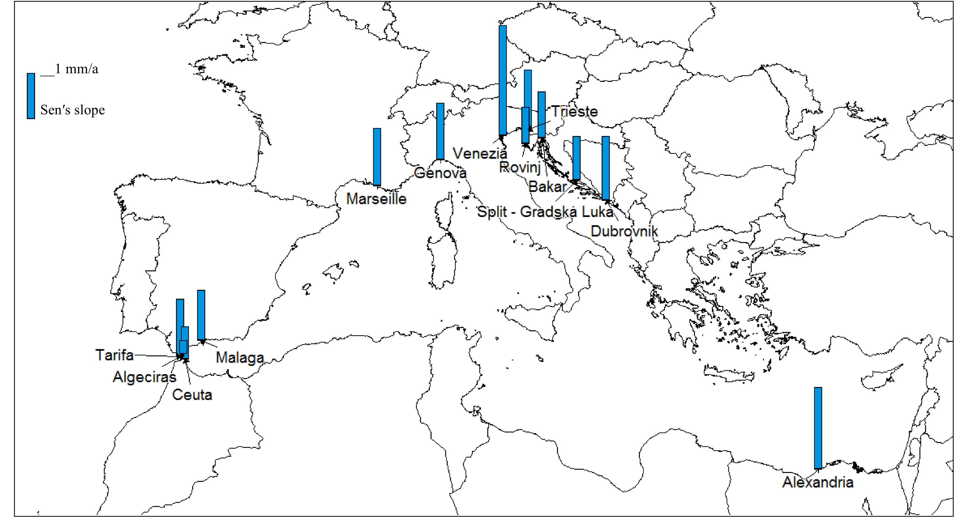
For illustrative purposes, Figure 2 displays the annual sea level trend at each station that has suitable data available over the selected period of more than 50 years.

Figure  2.  Geographic distribution of tide gauge stations and trends in mm/a.

DownLoad: Full-Size Img PowerPoint

5. Conclusions

The present study focuses on the investigation of the long term variability in the sea level along the Mediterranean shores. 14 long series of tidal heights, selected from the Permanent Sea Level Service (PSMSL) database, have been analyzed to find out their trends using the Mann-Kendall test and the Sen’s slope estimator. This comprises the stations of Tarifa (Spain), Algeciras (Spain), Malaga (Spain), Marseille (France), Genova (Italy), Venezia (Punta Della Salute) (Italy), Trieste (Italy), Rovinj (Croatia), Bakar (Croatia), Split Rt Marjana (Croatia), Split–Gradska Luka (Croatia), Dubrovnik (Croatia), Alexandria (Egypt) and Ceuta (Spain).

The obtained results show that the Split Rt Marjana series are the only one which do not exhibit a significant trend. The presence of a significant trend on this series is only evidenced by the use of seasonal Mann-Kendall test. This trend is not significant at the whole of the series; it is simply admissible from one month of January to the other, from one month of February to the next, and so on. The other 13 series showing significant trends are increasing, thus proving the rise of the Mediterranean Sea level.

After detecting the presence of significant and monotonic trends, the annual rates of sea level variability were estimated using the non-parametric seasonal Sen's approach. The overall estimated annual rates indicate a very net increase in the sea level along the Mediterranean shores. This result seems sufficient to suppose the presence, in the past century, of a new climatic phase on the scale of the Mediterranean basin, where the rising sea level is one of the consequences.

Faced with some emerging challenges associated with the climate change phenomenon, this study illustrates the effectiveness of the statistical tests for trend analysis of sea level time series. The results may seem primary, but these trends are of a crucial significance for climatologists for investigation into correlations between the major climatic events suffered by the Earth. As a matter of fact, the priorities for the improvements of this work will focuses on the possible interactions between the trend of the Mediterranean sea level with the climatic phenomena that may significantly affect its spatiotemporal variability, like the North Atlantic Oscillation and the Atlantic Multidecadal Oscillation.

Acknowledgements

We are enormously grateful to the Permanent Service of Mean Sea Level (PSMSL) for providing the sea level time series. We greatly thank the anonymous reviewers for their valuable and constructive comments.