Figure
1.
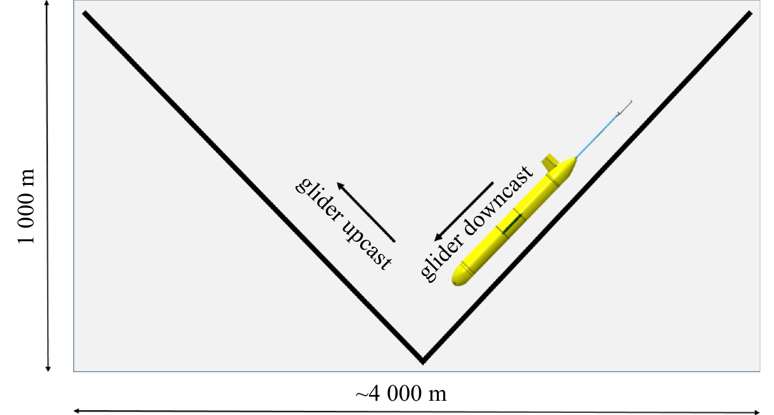
Schematic view of the Sea-Wing underwater glider sampling design.
| Citation: | Guifen Wang, Wen Zhou, Zhantang Xu, Wenlong Xu, Yuezhong Yang, Wenxi Cao. Vertical variations in the bio-optical properties of seawater in the northern South China Sea during summer 2008[J]. Acta Oceanologica Sinica, 2020, 39(4): 42-56. doi: 10.1007/s13131-020-1535-y

|
Underwater gliders are underwater autonomous vehicles first conceived and developed by Henry Stommel and Doug Webb in 1989 (Stommel, 1989). Gliders are able to follow a sawtooth pattern through a combination of vertical and horizontal movements based on a buoyance control system, adjustments in attitude, and adjustments of small fins (Rudnick et al., 2004; Garau et al., 2011). Glider vehicles are designed to autonomously dive to a water depth of typically up to 1 000 m and return to the sea surface along a predetermined path. During their diving and climbing stages, the vehicles observe the water column with various sensors equipped. Therefore, a specific glider mission often consists of several diving and climbing profiles (or downcasts and upcasts). Gliders currently serve as an important tool for oceanographic monitoring from coastal waters to open oceans owing to their capacity to operate autonomously in all weather conditions on missions lasting up to several months. Several commercial products, such as the Slocum glider manufactured by Teledyne Webb Research Corporation, Seaglider developed by the Applied Physics Laboratory at the University of Washington and now available through Kongsberg Maritime, and the Spray glider of the Scripps Institution of Oceanography and Bluefin Robotics, are now widely used in integrated ocean observing systems (e.g., United States Integrated Ocean Observing System (IOOS), Ocean Networks Canada, and the European Gliding Observatories Network), eddy monitoring from the sub-mesoscale to mesoscale (Ruiz et al., 2009; Bouffard et al., 2010, 2012; Baird et al., 2011), upper ocean monitoring from the hurricane pathway (Baltes et al., 2014; Miles et al., 2015), and providing high-resolution in-situ data to data assimilation and model forecasts (Shulman et al., 2009; Dobricic et al., 2010; Pan et al., 2011, 2014; Gangopadhyay et al., 2013; Dong et al., 2017).
In China, the development of the underwater glider began in 2003 and the first prototype named Sea-Wing was developed by the Shenyang Institute of Automation, Chinese Academy of Sciences (CAS) in 2005 (Yu et al., 2011). Another product is the Petrel underwater glider, developed by Tianjin University in 2009 (Liu et al., 2017). These two types of glider were adopted to monitor and understand the dynamics and structure of mesoscale eddies (Shu et al., 2016, 2018; Liu et al., 2019). Like the Slocum glider, both Sea-Wing and Petrel gliders have installed a Sea-Bird Glider Payload conductivity–temperature–depth (CTD) sensor (GPCTD hereafter), with a continuous sampling frequency of ~1 Hz.
Temperature and salinity are the most commonly used variables in oceanography. Temperature is observed directly with a specific sensor while salinity is calculated from measurements of conductivity and temperature using state equations (UNESCO, 1981). Like conventional CTD sensors, there is a misalignment in GPCTD sensor mounted on Sea-Wing gliders because the temperature and conductivity sensors are located downstream of one another, while the thermal inertia of the conductivity sensor introduces a cell thermal mass error in conductivity values and subsequently their derived parameters, such as water salinity and density. In other words, the conductivity cell has mass and the capacity to store heat and it therefore takes time for the conductivity sensor to adjust to the surrounding water, whereas the temperature sensor has a more rapid response time. Because conductivity is a strong function of temperature, a small change in water temperature inside the conductivity cell causes largely erroneous salinity values, especially across the thermocline. It is therefore important to conduct a thermal lag correction for both the downcast and upcast before using observations in scientific research. A practical method of correcting for heating inside the cell was developed by Morison et al. (1994). Garau et al. (2011) proposed a new method of correcting the thermal lag error associated with unpumped CTD sensors deployed on Slocum gliders. Liu et al. (2015) recently suggested practical procedures of correcting the thermal lag of salinity data recorded by an unpumped CTD sensor across a sharp thermocline.
Besides the thermal lag correction, a robust quality control (QC) procedure for temperature and salinity data obtained from gliders is also critical. The IOOS program drafted a real-time QC manual for CTD data obtained from gliders (U.S. Integrated Ocean Observing System, 2016), where a total of 19 tests are implemented. Tintoré et al. (2013) and Troupin et al. (2015) developed a Matlab-based glider toolbox (named the SOCIB Glider toolbox, https://github.com/socib/glider_toolbox) for processing glider data, correcting the thermal lag of salinity, and displaying data. However, like the CTD sensor mounted on Argo profiling floats, the CTD sensor, especially the conductivity sensor used on underwater gliders, may experience sensor drift owing to biofouling, biocide leakage into the conductivity cell, and a variety of other problems several months after their deployment (Wong et al., 2003; Oka and Ando, 2004; Liu et al., 2007). A comparison between the glider temperature and salinity profiles and a high-quality historical hydrographic data set or WOA climatology is thus necessary because profiles for which there has been sensor drift usually have good shapes and cannot be detected in real-time QC tests.
As technical development of the underwater glider progresses and the application of the underwater glider in oceanographic research and operational forecasts in China grows, the QC of data from either Sea-wing or Petrel gliders becomes increasingly important. On the basis of temperature and salinity profiles obtained by Sea-Wing underwater gliders, the present paper proposes a complete processing method that involves a thermal lag correction, real-time QC procedure involving 12 QC tests, and post-processing approach.
Three types of Sea-Wing underwater glider have been developed by the Shenyang Institute of Automation, CAS, namely 1 000-, 4 500-, and 7 000-m models. The present paper uses only the 1 000-m model because it has been more widely adopted than the other models in field investigations. The Sea-Wing glider has a mass of ~65 kg, a length of ~2 m, and the capacity to carry an additional ~3 kg of sensors. The glider is powered by batteries and can be deployed for up to 5 months, allowing 3 000 km of transections of water column (0−1 000 m) data to be sampled. The forward speed of the glider is approximately 0.3 m/s and varies depending on the predetermined path, mission duration, water density, and ocean front. The glider’s ascent/descent (Fig. 1) speeds vary through the water column depending on the glider’s buoyancy adjustment and attitude and the water density. With pressure and time data recorded on eight investigation cruises and by eight gliders between 2014 and 2016 in the South China Sea (SCS), the average descent/ascent speeds versus water pressure are estimated and shown in Fig. 2. It is clear that the descent speed is much more variable than the ascent speed, with the descent speed reaching a maximum value of 0.67 m/s around a depth of 50×104 Pa. The descent speed decreases rapidly between 50×104 and 200×104 Pa, where the pycnocline is located, and after that gliders maintain a mean descent speed of about 0.16 m/s until they reach their maximum profiling depth (~1 000 m). Meanwhile, the ascent speed is fairly stable, with an average value of about 0.23 m/s. A Sea-Wing glider takes approximately 1.85 h on average to dive from the sea surface to a depth of 1 000 m and 1.49 h to climb from a depth of 1 000 m to the sea surface.

Each Sea-Wing glider is installed with a Sea-Bird GPCTD sensor. Considering the data transmission rate, Sea-Wing gliders are currently programmed to record a CTD sample for a 6-s interval. When a CTD sample is required, the GPCTD pump turns on and produces a constant flow rate of ~0.01 L/s; i.e., the speed of the flow through the temperature sensor and conductivity cell is fixed and known, which makes the thermal lag correction more effective than that for unpumped CTDs (e.g., SBE41 CTD), where the flow rate varies depending on the angle and speed of the glider (Liu et al., 2015).
Pressure, temperature, and conductivity measurements and associated time information are reported by Sea-Wing gliders. In addition, a Global Positioning System (GPS) fix and time stamp is obtained when the glider starts to dive or reaches the sea surface from underwater. A precise duration calculation often applies the UNIX epoch, which is the number of seconds that have elapsed since 1 January 1970 (midnight UTC/GMT). Therefore, all the date and time information for both CTD measurements and GPS fixes are converted into the UNIX epoch time before processing.
Because sea water salinity is computed from the conductivity, temperature, and pressure measured by a GPCTD sensor on the Sea-Wing glider, it is necessary to detect and exclude abnormal conductivity induced by the behavior of the glider or biofouling on the CTD sensor. When a glider starts to dive or ends its ascending profile, the CTD sensor mounted may be exposed to the air and record abnormal conductivity data. Three QC tests are conducted to detect erroneous conductivity measurements.
(1) Global range test
The global range test is conducted to detect erroneous conductivity values out of the range of the measurement range of the conductivity sensor; i.e., 0−6 S/m. If any conductivity value fails this test, the conductivity value and its corresponding temperature value are flagged as bad data (“4”) and excluded from the further calculation of salinity.
(2) Spike test
Prior to the spike test, the descent and ascent phases of a glider cycle are split into a downcast and upcast. The spike test does not consider differences in pressure but assumes a sampling that adequately reproduces changes in conductivity with pressure. The conductivity value
| $$ \begin{split} & \left| {C\left( i \right) - \left( {C\left( {i + 1} \right) + C\left( {i - 1} \right)} \right)/2} \right|-\\ & \left| {\left( {C\left( {i + 1} \right) - C\left( {i - 1} \right)} \right)/2} \right| > K, \end{split} $$ | (1) |
where
(3) Running standard-deviation test
The running standard-deviation algorithm is taken from the United States IOOS Glider DAC QC manual. The values of the running average (Cave(i)) and standard deviation (Cstd(i)) over nine consecutive points (if not previously flagged as bad) are computed for each i = 4 to N − 3 (where N is the total number of points in a profile). The preceding and succeeding points are not used in the calculation if the time interval between adjacent points is greater than 30 s or the depth interval is greater than 5×10⁴ Pa. For the first (last) four points of the time series, the average and standard deviation are computed as for the fifth (N−4th) value.
A conductivity value should be flagged as bad if not previously flagged and both
A thermal lag correction should be applied prior to the QC of the glider observations. A Matlab script from the SOCIB Glider toolbox is employed for the thermal lag correction of Sea-Wing gliders installed with a GPCTD sensor. This script adopts the approach developed by Lueck and Picklo (1990). They expressed the conductivity correction (
| $${C_T}\left( n \right) = - b{C_T}\left( {n - 1} \right) + \gamma a\left[ {T\left( n \right) - T\left( {n - 1} \right)} \right], $$ | (2) |
where
| $$ {\rm{}}a = \frac{{4{f_n}\alpha \tau }}{{1 + 4{f_n}\tau }}, $$ | (3) |
| $$ b = \frac{{1 - 2a}}{\alpha }, $$ | (4) |
where
| $$ \alpha = 0.013\;5 + 0.026\;4/V, $$ | (5) |
| $$ \tau = 7.149\;9 + 2.785\;8/\sqrt V , $$ | (6) |
where
| $$ \alpha \left( n \right) = {\alpha _o} + {a_s}/V\left( n \right), $$ | (7) |
| $$ \tau \left( n \right) = {\tau _o} + {\tau _s}/\sqrt {V\left( n \right)} , $$ | (8) |
where the subscripts
Conductivity is a strong function of temperature as mentioned above, and an increasing mismatch between the temperature in the conductivity cell and ambient water therefore leads to a remarkable salinity error. To illustrate the thermal lag effect in different water columns, we selected three profiles (downcast and upcast) recorded by GPCTD sensors on two Sea-Wing gliders (Fig. 3). The downcast and upcast of each profile were observed within 3 km spatially and 4 h temporally. Figures 3a−c presents observations obtained by Glider 1000J003 operating in the SCS on 5 July 2016 under conditions of a relatively weak thermocline (the average temperature gradient was 0.09°C/m between 20×104 and 80×104 Pa) and shallow mixed layer depth (MLD) of ~20×104 Pa. No thermal lag effect is evident, and the salinity difference between the downcast and upcast is only ~0.05 between 60×104 and 180×104 Pa. Figures 3d−f presents observations obtained by the same glider except that the profile was observed in the northern SCS on 8 May 2015. In this case, the thermocline is stronger with an average temperature gradient of about 0.13°C/m in the range of 20×104−80×104 Pa. A salinity difference between the downcast and upcast is evident above a depth of 200×104 Pa, with the difference being a maximum of ~0.35 around a depth of 50×104 Pa (Fig. 3e). The salinities from the downcast are higher than those from the upcast between 30×104 and 200×104 Pa. This appreciable salinity difference is obviously induced by the thermal lag effect and larger temperature gradients when the glider crosses the thermocline. Using the Matlab script from the SOCIB Glider toolbox, the thermal lag was corrected with an initial guess for

Statistically, below the mixed layer, the downcast salinities after thermal lag correction are lower than the raw salinities directly computed from the reported conductivities (Fig. 4). In particular, the amplitude of the correction can be larger than 0.1 at water depths of 50×104 −60×104 Pa with strong temperature gradients. In contrast, the upcast salinities after thermal lag correction are generally higher than the raw salinities throughout the water column, but the amplitude of the correction across a strong temperature gradient is much smaller than that for the downcast. The reason why the thermal lag effect is more remarkable for the downcast is not clear and requires further investigation.

Because the underwater glider has a mission schematic and CTD sensor similar to those of the Argo profiling float, the real-time QC tests being applied to Argo can also be adopted for gliders; e.g., the United States IOOS Glider data assembly center (DAC) has developed QC tests referring to Argo (U.S. Integrated Ocean Observing System, 2016). In the real-time QC of Argo CTD data, about 16 tests are automatically conducted by computers, including tests for the profile location, date and time, drifting speed, density inversion, stuck values, global/regional range, deepest pressure, spikes, and gradients of temperature and salinity profiles (Wong et al., 2019). It is worth noting that a climatological test strongly recommended by the glider community has not yet been adopted in Argo real-time QC, probably because delayed-mode QC methods (Wong et al., 2003; Böhme and Send, 2005; Owens and Wong, 2009) have been adopted to calibrate Argo salinity profiles using a global high quality and high-resolution hydrographic data set. However, in our work, when we develop a real-time QC tool for Sea-Wing gliders, a climatological test is considered together with Argo-equivalent QC tests.
(1) Date test
The date test requires that the Julian day (JULD) of a glider downcast/upcast profile be later than 1 January 2010 and earlier than the current date of the check (in UTC time). If JULD denotes the number of days that have elapsed since 1 January 1970, then the date of a glider profile fails the test when JULD < 14 610 or JULD > UTC date of the test. The date of the profile is flagged as bad data (“4”) and none of the data from the profile are used.
(2) Position test
First, the observation latitude and longitude of a glider profile should be between −90° and 90° and between −180° and 180° respectively. If either the latitude or longitude fails this test, the profile position is flagged as bad data and none of the data from the profile are used.
Second, the profile position should be located in an ocean. We make use of the global 5-min bathymetry data set (ETOPO5/TerrainBase), which can be downloaded from http://iridl.ldeo.columbia.edu/SOURCES/.NOAA/.NGDC/.ETOPO5/datasetdatafiles.html. If a position cannot be located in an ocean, the profile is flagged as bad data.
(3) Pressure test
All pressure measurements in seawater should be larger than 0 Pa. If any pressure fails this test, the pressure and its corresponding temperature and salinity are flagged as bad data. In addition, if we know the preprogrammed maximum profiling depth (DEEPEST_PRES) of an underwater glider, a deepest-pressure test can be conducted as no pressure measurement of a profile should be greater than 1.1 × DEEPEST_PRES.
(4) Global range test
A gross filter is applied to observations of temperature and salinity. The ranges need to accommodate all expected extremes that may occur in the oceans; i.e., temperatures in the range of −2.5 to 40.0°C and salinity in the range of 0 to 41.
(5) Stuck profile test
The stuck profile test looks for measurements of temperature and salinity in a profile being identical. Each point in a profile is flagged as bad if the difference between the minimum and maximum values on the profile is less than the resolution of the CTD sensor; i.e., max(T(i)) − min(T(i)) < 0.001°C and max(S(i)) − min(S(i)) < 0.001, where T and S are respectively the temperature and salinity, and i is the start-to-end array index of the profile.
(6) Spike test
The spike test uses the same algorithm as that used for conductivity; i.e., Eq. (1).
For temperature (T(i)):
temp_flag(i) = 4 if not previously flagged and
| $$ \begin{split} & \left| {T\left( i \right) - \left( {T\left( {i + 1} \right) + T\left( {i - 1} \right)} \right)/2} \right| -\\ & \left| {\left( {T\left( {i + 1} \right) - T\left( {i - 1} \right)} \right)/2} \right|>K, \end{split} $$ | (9) |
where K = 6°C (Z(i) < 500×104 Pa) or K = 2°C (Z(i) ≥ 500×104 Pa) and Z is the pressure.
For salinity (S(i)):
salt_flag(i) = 4 if not previously flagged and
| $$ \begin{split} & \left| {S\left( i \right) - \left( {S\left( {i + 1} \right) + S\left( {i - 1} \right)} \right)/2} \right| -\\ & \left| {\left( {S\left( {i + 1} \right) - S\left( {i - 1} \right)} \right)/2} \right| >K, \end{split} $$ | (10) |
where K = 1.0 (Z(i) < 500×104 Pa) or K = 0.5 (Z(i) ≥ 500×104 Pa).
(7) Gradient test
The gradient test is failed when the difference between vertically adjacent measurements is too great. The test does not consider differences in pressure but assumes a sampling that adequately reproduces changes in temperature and salinity with pressure. The algorithm from the United States IOOS Glider DAC QC manual (U.S. Integrated Ocean Observing System, 2016) is adopted here.
For temperature:
temp_flag(i) = 4 and temp_flag(i+1) = 4 if not previously flagged and
| $$ \left| {\left( {T\left( {i + 1} \right) - T\left( i \right)} \right)/\left( {Z\left( {i + 1} \right) - Z\left( i \right)} \right)} \right|>K, $$ | (11) |
where K = 2°C/104 Pa (Z(i+1) ≤ 5×10⁴ Pa), K = 8°C/104 Pa (5×10⁴ Pa < Z(i+1) ≤ 500×104 Pa), K = 2°C/104 Pa (Z(i+1) > 500×104 Pa).
For salinity:
salt_flag(i) = 4 and salt_flag(i+1) = 4 if not previously flagged and
| $$ \left| {\left( {S\left( {i + 1} \right) - S\left( i \right)} \right)/\left( {Z\left( {i + 1} \right) - Z\left( i \right)} \right)} \right|>K, $$ | (12) |
where K = 0.3/104 Pa (Z(i+1) ≤ 5×10⁴ Pa), K = 1.7/×104 Pa (5×10⁴ Pa < Z(i+1) ≤ 500×104 Pa), K = 0.15/104 Pa (Z(i+1) > 500×104 Pa).
(8) Running standard-deviation test
The running standard-deviation test employs the same algorithm as that used for conductivity in Section 3.2.
For temperature:
temp_flag(i) = 4 if not previously flagged and both
For salinity:
salt_flag(i) = 4 if not previously flagged and both
(9) Racape’s spike test
A new spike test is based on the method presented by Racape et al. (2018) at the 19th meeting of the Argo data management team (San Diego, U.S.A., December 2018) and is expected to be applied to Argo real-time QC in the future. In the method, a five-point moving median is suggested and computed along the entire profile (while the median value is computed if there are fewer than five points). If the difference between the observed value and its associated moving median is greater than a given standard deviation, the value is flagged as bad data (“4”). The thresholds of the temperature and salinity standard deviations depend on depth and have spatiotemporal variability. One can compute a global-ocean monthly temperature and salinity standard deviation climatology using the WOA or other datasets. We here use thresholds similar to those given by Racape et al. (2018) as shown in Table 1. Figure 5 shows an example of the test for a given salinity profile. Two successive salinity anomalies around a depth of 500×104 Pa and three at depths between 700×104 and 800×104 Pa are defined manually prior to testing. Results show that Racape’s spike test screened the former two successive anomalies successfully but failed to screen the latter three successive anomalies. The new spike test is thus limited and can detect no more than two successive spikes efficiently.

(10) Density inversion test
Before the density inversion test, the potential density is computed using the Matlab seawater toolbox (http://www.cmar.csiro.au/datacentre/ext_docs/seawater.htm). From top to bottom, if the potential density calculated at the greater pressure Z(i+1) is less than that calculated at the lesser pressure Z(i) by more than 0.03 kg/m3, both the temperature and salinity values at Z(i) and Z(i+1) are flagged as bad data.
(11) Vertical velocity test
Figure 2 shows that the vertical speed of a Sea-Wing glider is no lower than 0.1 m/s on average. We define 0.03 m/s as the threshold of vertical velocity, and any pressure, temperature, and salinity measurements excluding data shallower than 10×104 Pa and 10×104 Pa shallower than the maximum profiling depth should be flagged as bad data if the calculated vertical velocity is less than 0.03 m/s. This test ensures that observations made by a Sea-Wing glider are obtained during a period of good behavior and pitch change of the glider.
(12) Climatological test
A climatological test is strongly recommended for the real-time QC of gliders because a sensor on a glider may drift several months after the glider’s deployment. This sensor drift usually results in a systematic error in the temperature or salinity profile that is difficult to detect in Argo-equivalent QC tests. A good climatology data set can be used to visually inspect the quality of temperature and salinity profiles and detect potential sensor drift. We here choose the historical hydrographic data set maintained by the Coriolis data center (IFREMER) as the climatology data set that we will apply in the glider climatological test. Each shipboard CTD profile contained in the data set has been visually checked by the operator at the Coriolis data center. The data set (named the DMQC_Argo CTD dataset) is not publicly available and can only be used in Argo delayed-mode QC. In addition, considering the many gaps, especially in the Southern Ocean (Fig. 6), we downloaded the WOA2018 climatology (Garcia et al., 2019) as an alternative to the DMQC_Argo CTD dataset. However, a global climatology data set usually has many profiles, which reduces the search speed when we conduct a climatological test for profiles one by one. We therefore separated both the DMQC_Argo CTD and WOA18 data sets into many small boxes (10° × 10°), which is expected to accelerate our data search.

The temperature/salinity mean and standard deviation are calculated as functions of the standard depth for the DMQC_Argo CTD data set using all the temperature/salinity profiles in each box, whereas existing standard deviations in the WOA18 are directly used. In the climatological test for our glider, according to the GPS fix of a downcast/upcast profile, a corresponding box is searched for either from the DMQC_Argo CTD or WOA18. Both the temperature and salinity standard-deviation profiles are linearly interpolated to the glider’s vertical level. The glider-observed profile and mean climatological profile are then compared. If the difference between the two profiles is larger than n_std × Qstd(i), then the corresponding value should be flagged as doubtable (‘3’), where Qstd(i) is the temperature or salinity standard deviation from the DMQC_Argo_CTD or WOA18 that we have interpolated to the glider’s level and n_std is the multiple factor of the standard deviation that gives the threshold. A robust choice of n_std is expected to accommodate seasonal and long-term ocean variability on a basin scale. The selection of n_std should therefore be made cautiously, which requires the local QC operator to know the regional ocean variability. According to the United States Navy’s standard monthly ocean temperature and salinity climatology (GDEM), n_std = 5 was previously used for the United States IOOS Glider DAC, but there were too many cases in which this test was failed even though the temperature and salinity were apparently good (U.S. Integrated Ocean Observing System, 2016). In our work, a larger threshold in the range of 6 to 8 is recommended.
Figure 7 presents an example of the climatological test using temperature and salinity profiles obtained from an Argo profiling float (WMO number: 2902581; cycle number: 93). We did not use data from Sea-Wing gliders because we have not found a profile from the existing glider data set that both contains sensor drift and has good shape. It is clearly seen that the salinity profile of the 93th cycle has a systematic offset against the other profiles (Fig. 7a), which is probably due to biofouling or other technical problems. The entire temperature profile falls into the climatological standard-deviation envelop with n_std = 6 (Fig. 7c), while part of the salinity data fails the test between 400×104 and 2 000×104 Pa, suggesting that the salinity data from this float contain a positive sensor drift or offset.

After correcting for thermal lag and conducting the 12 proposed real-time QC tests, the data are clearer and more consistent between downcast and upcast profiles than the raw data. However, mismatches between the downcast and upcast profiles, especially across the thermocline, are not completely eliminated (Fig. 8). The corrected temperature data in the downcast profile tend to be lower than those in the upcast profile. Conversely, the corrected salinity data in the downcast profile are higher than those in the upcast profile. A simple average taken between the downcast and upcast profiles thus seems to be more reasonable if we consider that the two profiles should measure the same water mass. Meanwhile, even large spikes should have been removed by the two spike tests in Section 3.4 and yet small hooks are found in both the temperature and salinity profiles (not shown). To remove these hooks, a moving (five-point) mean filter is strongly suggested before averaging. Afterward, both the corrected downcast and upcast temperature/salinity profiles are first linearly interpolated to the same vertical levels. The two interpolated profiles are then averaged into one single profile. The effect of the moving mean filter and averaging is seen in Fig. 8 (blue lines). In order to illustrate the amplitude of the salinity difference between post-processed and corresponding corrected downcast/upcast profiles, we selected all observations (1 566 profiles in total) from three gliders (1000J001−003) that operated in the SCS. It can be seen from Fig. 9 that the mean salinity differences between post-processed and corrected downcast are almost within ±0.1. The most notable differences are found at depths of 40×104−60×104 Pa(with the maximum standard deviation being as high as 0.08 for Glider 1000J002), where temperature gradients are strongest. These differences are negligible below 150×104 Pa. The upcast profiles have the similar post-processed−corrected salinity differences as the downcast profiles but show an inverse distribution in vertical (not shown)


The real-time QC of CTD profiles recorded by underwater gliders usually involves a thermal lag correction, various QC tests (similar to Argo real-time QC tests), and the post-processing of downcast and upcast profiles. Thermal lag effects are generated by the mismatch between the temperature probe and conductivity cell response times. Such a thermal lag effect is more evident when a glider crosses a sharp temperature gradient (strong thermocline). Because the conductivity strongly depends on temperature, the reported thermal-lag-induced salinity error can be up to ~0.3 for a strong thermocline. Without correction of the thermal lag, salinity profiles derived from conductivity observations will contain large errors, especially profiles in areas having a strong thermocline. The correction of the thermal lag effect relies on the flow speed through the conductivity cell. The use of a CTD sensor without a pump system (i.e., an unpumped system) leads to a variable flow speed owing to the variable glider surge speed, which is thought to introduce difficulties to the thermal lag correction. It is therefore strongly recommended that a CTD sensor with a pump system (e.g., a GPCTD or SBE41CP) is installed on a glider. In addition, a high-resolution sampling scheme is required in an area having a sharp thermocline for the better correction of thermal lag. As for a Sea-Wing glider installed with a GPCTD (having a sampling rate of ~1 Hz), we suggest the manufacturer design the glider to record and transmit all original samples instead of subsamples.
It is worth noting that the CTD sensor mounted on a glider can be calibrated in the laboratory either prior to its deployment or after its recovery in contrast to the case of a sensor mounted on an (expendable) autonomous profiling float, which is expected to favor the QC of observations. However, gliders are often deployed in coastal waters, where their sensors are inevitably affected by oil contamination or biofouling. This puts more focus on the QC of their observations than on the QC of the observations of autonomous profiling floats. In particular, the systematic error of each CTD sensor should be known in an observation network comprising tens of co-operating gliders. Besides sensor calibration in the laboratory, in-situ comparisons with shipboard CTD casts and analyses conducted using a salinometer are critical. In addition, the establishment of a regional high-quality hydrographic data set is essential to detect sensor drift that may occasionally occur for gliders. We also suggest that the Argo-equivalent target accuracy (i.e., 0.01 for salinity, 0.005℃ for temperature and 2.5×10⁴ Pa for pressure) be adopted for gliders in open oceans and some marginal seas, such as the South China Sea.
As the use of CTD data recorded by Sea-Wing gliders increases, an approach for processing these data becomes necessary. It will be meaningful to draft a QC manual and develop a robust toolbox for both the processing and real-time QC of CTD observations made by gliders.
The present paper, on the basis of observations made by Sea-Wing gliders, proposed a complete real-time QC procedure of CTD profiles, involving thermal lag correction, 12 QC tests, and a simple post-processing method. Among the real-time QC tests, a new spike test based on the method proposed by Racape and a climatological test using a high-quality historical hydrographic data set (DMQC_Argo CTD) previously used for Argo delayed-mode QC and WOA climatology were first suggested. The climatological test can be used to detect potential sensor drift given an appropriate threshold (n_std times the standard deviation). It is noted that the behaviors of a glider are also important in determining the glider’s vertical velocity and thus the quality of the temperature and salinity profiles. These QC tests could also be adopted for Petrel gliders.
This work benefited from numerous freely available data sets and useful toolboxes. The Sea-Wing underwater glider data were provided by the State Key Laboratory of Robotics, Shenyang Institute of Automation, Chinese Academy of Sciences. The WOA2018 climatology was developed by the National Centers for Environmental Information, NOAA and downloaded from https://www.nodc.noaa.gov/OC5/woa18. The DMQC_Argo CTD data set was provided by the Coriolis data center (IFREMER). The Matlab scripts for the thermal lag correction were taken from the SOCIB Glider toolbox (https://github.com/socib/glider_toolbox). The Matlab seawater toolbox was provided by CSIRO, Australia (http://www.cmar.csiro.au/datacentre/ext_docs/seawater.htm). We thank Glenn Pennycook, MSc, from Liwen Bianji, Edanz Group China (www.liwenbianji.cn/ac), for editing the English text of a draft of this manuscript.
| [1] |
Barnard A H, Pegau W S, Zaneveld J R V. 1998. Global relationships of the inherent optical properties of the oceans. Journal of Geophysical Research, 103(C11): 24955–24968. doi: 10.1029/98JC01851
|
| [2] |
Behrenfeld M J, Boss E. 2003. The beam attenuation to chlorophyll ratio: an optical index of phytoplankton physiology in the surface ocean?. Deep Sea Research Part I: Oceanographic Research Papers, 50(12): 1537–1549. doi: 10.1016/j.dsr.2003.09.002
|
| [3] |
Behrenfeld M J, Boss E, Siegel D A, et al. 2005. Carbon-based ocean productivity and phytoplankton physiology from space. Global Biogeochemical Cycles, 19(1): GB1006
|
| [4] |
Bishop J K B. 1999. Transmissometer measurement of POC. Deep Sea Research Part I: Oceanographic Research Papers, 46(2): 353–369. doi: 10.1016/S0967-0637(98)00069-7
|
| [5] |
Boss E S, Collier R, Larson G, et al. 2007. Measurements of spectral optical properties and their relation to biogeochemical variables and processes in Crater Lake, Crater Lake National Park, OR. Hydrobiologia, 574(1): 149–159. doi: 10.1007/s10750-006-2609-3
|
| [6] |
Boss E, Pegau W S, Gardner W D, et al. 2001. Spectral particulate attenuation and particle size distribution in the bottom boundary layer of a continental shelf. Journal of Geophysical Research: Oceans, 106(C5): 9509–9516. doi: 10.1029/2000JC900077
|
| [7] |
Boss E, Picheral M, Leeuw T, et al. 2013. The characteristics of particulate absorption, scattering and attenuation coefficients in the surface ocean; Contribution of the Tara Oceans expedition. Methods in Oceanography, 7: 52–62. doi: 10.1016/j.mio.2013.11.002
|
| [8] |
Brewin R J W, Dall’Olmo G, Pardo S, et al. 2016. Underway spectrophotometry along the Atlantic Meridional Transect reveals high performance in satellite chlorophyll retrievals. Remote Sensing of Environment, 183: 82–97. doi: 10.1016/j.rse.2016.05.005
|
| [9] |
Buesseler K O. 2001. Ocean biogeochemistry and the global carbon cycle: an introduction to the U.S. joint global ocean flux study. Oceanography, 14(4): 5. doi: 10.5670/oceanog.2001.01
|
| [10] |
Chang G C, Dickey T D. 2001. Optical and physical variability on timescales from minutes to the seasonal cycle on the New England shelf: July 1996 to June 1997. Journal of Geophysical Research: Oceans, 106(C5): 9435–9453. doi: 10.1029/2000JC900069
|
| [11] |
Chen C C, Shiah F K, Chung S W, et al. 2006. Winter phytoplankton blooms in the shallow mixed layer of the South China Sea enhanced by upwelling. Journal of Marine Systems, 59(1–2): 97–110. doi: 10.1016/j.jmarsys.2005.09.002
|
| [12] |
Claustre H, Fell F, Oubelkheir K, et al. 2000. Continuous monitoring of surface optical properties across a geostrophic front: Biogeochemical inferences. Limnology and Oceanography, 45(2): 309–321
|
| [13] |
Cui Wansong, Wang Difeng, Gong Fang, et al. 2016. The vertical distribution of the beam attenuation coefficient and its correlation to the particulate organic carbon in the north South China Sea. In: Remote Sensing of the Ocean, Sea Ice, Coastal Waters, and Large Water Regions. Edinburgh, United Kingdom: SPIE, 2016
|
| [14] |
Cullen J J. 1982. The deep chlorophyll maximum: Comparing vertical profiles of chlorophyll a. Canadian Journal of Fisheries and Aquatic Sciences, 39(5): 791–803. doi: 10.1139/f82-108
|
| [15] |
Cullen J J. 2015. Subsurface chlorophyll maximum layers: Enduring enigma or mystery solved?. Annual Review of Marine Science, 7: 207–239. doi: 10.1146/annurev-marine-010213-135111
|
| [16] |
Dickey T D. 2001. The role of new technology in advancing ocean biogeochemical research. Oceanography, 14(4): 108–120. doi: 10.5670/oceanog.2001.11
|
| [17] |
Fennel K, Boss E. 2003. Subsurface maxima of phytoplankton and chlorophyll: Steady-state solutions from a simple model. Limnology and Oceanography, 48(4): 1521–1534. doi: 10.4319/lo.2003.48.4.1521
|
| [18] |
Fujii M, Boss E, Chai F. 2007. The value of adding optics to ecosystem models: a case study. Biogeosciences, 4(5): 817–835. doi: 10.5194/bg-4-817-2007
|
| [19] |
Gardner W D, Gundersen J S, Richardson M J, et al. 1999. The role of seasonal and diel changes in mixed-layer depth on carbon and chlorophyll distributions in the Arabian Sea. Deep Sea Research Part II: Topical Studies in Oceanography, 46(8–9): 1833–1858. doi: 10.1016/S0967-0645(99)00046-6
|
| [20] |
Gernez P, Antoine D, Huot Y. 2011. Diel cycles of the particulate beam attenuation coefficient under varying trophic conditions in the northwestern Mediterranean Sea: Observations and modeling. Limnology and Oceanography, 56(1): 17–36. doi: 10.4319/lo.2011.56.1.0017
|
| [21] |
Gong Xiang, Shi Jie, Gao Huiwang, et al. 2014. Modeling seasonal variations of subsurface chlorophyll maximum in South China Sea. Journal of Ocean University of China, 13(4): 561–571. doi: 10.1007/s11802-014-2060-4
|
| [22] |
Gong Xiang, Shi Jinhui, Gao Huiwang, et al. 2015. Steady-state solutions for subsurface chlorophyll maximum in stratified water columns with a bell-shaped vertical profile of chlorophyll. Biogeosciences, 12(4): 905–919. doi: 10.5194/bg-12-905-2015
|
| [23] |
Kara A B, Rochford P A, Hurlburt H E. 2000. An optimal definition for ocean mixed layer depth. Journal of Geophysical Research, 105(C7): 16803–16821. doi: 10.1029/2000JC900072
|
| [24] |
Kheireddine M, Antoine D. 2014. Diel variability of the beam attenuation and backscattering coefficients in the northwestern Mediterranean Sea (BOUSSOLE site). Journal of Geophysical Research: Oceans, 119(8): 5465–5482. doi: 10.1002/2014JC010007
|
| [25] |
Kitchen J C, Zaneveld J R V. 1990. On the noncorrelation of the vertical structure of light scattering and chlorophyll α in case I waters. Journal of Geophysical Research: Oceans, 95(C11): 20237–20246. doi: 10.1029/JC095iC11p20237
|
| [26] |
Knap A, Michaels A, Close A, et al. 1996. Protocols for the Joint Global Ocean Flux Study (JGOFS) core measurements. Reprint of the IOC Manuals and Guides No. 29, UNESCO, Paris
|
| [27] |
Lavigne H, D’Ortenzio F, D’Alcalà M R, et al. 2015. On the vertical distribution of the chlorophyll a concentration in the Mediterranean Sea: a basin-scale and seasonal approach. Biogeosciences, 12(16): 5021–5039. doi: 10.5194/bg-12-5021-2015
|
| [28] |
Li Q P, Dong Y, Wang Y. 2016. Phytoplankton dynamics driven by vertical nutrient fluxes during the spring inter-monsoon period in the northeastern South China Sea. Biogeosciences, 13: 455–466. doi: 10.5194/bg-13-455-2016
|
| [29] |
Li Q P, Franks P J S, Landry M R, et al. 2010. Modeling phytoplankton growth rates and chlorophyll to carbon ratios in California coastal and pelagic ecosystems. Journal of Geophysical Research, 115(G4): G04003
|
| [30] |
Lin Junfang, Cao Wenxin, Wang Guifen, et al. 2014. Inversion of bio-optical properties in the coastal upwelling waters of the northern South China Sea. Continental Shelf Research, 85: 73–84. doi: 10.1016/j.csr.2014.06.001
|
| [31] |
Lin Peigen, Cheng Peng, Gan Jianping, et al. 2016. Dynamics of wind-driven upwelling off the northeastern coast of Hainan Island. Journal of Geophysical Research: Oceans, 121(2): 1160–1173. doi: 10.1002/2015JC011000
|
| [32] |
Liu K K, Chao S Y, Shaw P T, et al. 2002. Monsoon-forced chlorophyll distribution and primary production in the South China Sea: observations and a numerical study. Deep Sea Research Part I: Oceanographic Research Papers, 49(8): 1387–1412. doi: 10.1016/S0967-0637(02)00035-3
|
| [33] |
Liu Fenfen, Tang Shilin, Chen Chuqun. 2013. Impact of nonlinear mesoscale eddy on phytoplankton distribution in the northern South China Sea. Journal of Marine Systems, 123–124: 33–40. doi: 10.1016/j.jmarsys.2013.04.005
|
| [34] |
Lu Zhongming, Gan Jianping, Dai Minhan, et al. 2010. The influence of coastal upwelling and a river plume on the subsurface chlorophyll maximum over the shelf of the northeastern South China Sea. Journal of Marine Systems, 82(1–2): 35–46. doi: 10.1016/j.jmarsys.2010.03.002
|
| [35] |
Ma Jinfeng, Zhan Haigang, Du Yan. 2011. Seasonal and interannual variability of surface CDOM in the South China Sea associated with El Niño. Journal of Marine Systems, 85(3–4): 86–95. doi: 10.1016/j.jmarsys.2010.12.006
|
| [36] |
McGillicuddy D J Jr. 2016. Mechanisms of physical-biological-biogeochemical interaction at the oceanic mesoscale. Annual Review of Marine Science, 8(1): 125–159. doi: 10.1146/annurev-marine-010814-015606
|
| [37] |
McGillicuddy D J Jr, Johnson R, Siegel D A, et al. 1999. Mesoscale variations of biogeochemical properties in the Sargasso Sea. Journal of Geophysical Research: Oceans, 104(C6): 13381–13394. doi: 10.1029/1999JC900021
|
| [38] |
Mignot A, Claustre H, D’Ortenzio F, et al. 2011. From the shape of the vertical profile of in vivo fluorescence to Chlorophyll-a concentration. Biogeosciences, 8(8): 2391–2406. doi: 10.5194/bg-8-2391-2011
|
| [39] |
Mignot A, Claustre H, Uitz J, et al. 2014. Understanding the seasonal dynamics of phytoplankton biomass and the deep chlorophyll maximum in oligotrophic environments: A Bio-Argo float investigation. Global Biogeochemical Cycles, 28(8): 856–876. doi: 10.1002/2013GB004781
|
| [40] |
Mitchell B G, Kahru M, Wieland J, et al. 2003. Determination of spectral absorption coefficients of particles, dissolved material and phytoplankton for discrete water samples. In: Mueller J L, Fargoin G S, McClain C R, eds. Ocean Optics Protocols for Satellite Ocean Color Sensor Validation, revision 4, Vol. IV (Chapter 4), NASA/TM-2003-211621/Rev4-vol. 4. Greenbelt, MD: NASA Goddard Space Flight Center, 39–64
|
| [41] |
Mobley C D. 1994. Light and Water: Radiative Transfer in Natural Waters. San Diego, CA, USA: Academic Press
|
| [42] |
Morel A. 1988. Optical modeling of the upper ocean in relation to its biogenous matter content (case I waters). Journal of Geophysical Research: Oceans, 93(C9): 10749–10768. doi: 10.1029/JC093iC09p10749
|
| [43] |
Morel A, Maritorena S. 2001. Bio-optical properties of oceanic waters: A reappraisal. Journal of Geophysical Research: Oceans, 106(C4): 7163–7180. doi: 10.1029/2000JC000319
|
| [44] |
Nencioli F, Chang G, Twardowski M, et al. 2010. Optical characterization of an eddy-induced diatom bloom west of the island of Hawaii. Biogeosciences, 7(1): 151–162. doi: 10.5194/bg-7-151-2010
|
| [45] |
Ning Xiuren, Chai Fei, Xue Huijie, et al. 2004. Physical-biological oceanographic couplinginfluencing phytoplankton and primary production in the South China Sea. Journal of Geophysical Research: Oceans, 109: C10005. doi: 10.1029/2004JC002365
|
| [46] |
Oubelkheir K, Claustre H, Sciandra A, et al. 2005. Bio-optical and biogeochemical properties of different trophic regimes in oceanic waters. Limnology and Oceanography, 50(6): 1795–1809. doi: 10.4319/lo.2005.50.6.1795
|
| [47] |
Oubelkheir K, Sciandra A. 2008. Diel variations in particle stocks in the oligotrophic waters of the Ionian Sea (Mediterranean). Journal of Marine Systems, 74(1–2): 364–371. doi: 10.1016/j.jmarsys.2008.02.008
|
| [48] |
Pan Xiaoju, Wong G T F, Tai J H, et al. 2015. Climatology of physical hydrographic and biological characteristics of the Northern South China Sea Shelf-sea (NoSoCS) and adjacent waters: Observations from satellite remote sensing. Deep Sea Research Part II: Topical Studies in Oceanography, 117: 10–22. doi: 10.1016/j.dsr2.2015.02.022
|
| [49] |
Parsons T, Takahashi M, Hargrave B. 1984. Biological Oceanographic Processes. 3rd ed. England: Pergamon Press, 330
|
| [50] |
Pérez V, Fernández E, Marañón E, et al. 2006. Vertical distribution of phytoplankton biomass, production and growth in the Atlantic subtropical gyres. Deep Sea Research Part I: Oceanographic Research Papers, 53(10): 1616–1634. doi: 10.1016/j.dsr.2006.07.008
|
| [51] |
Platt T, Bouman H, Devred E, et al. 2005. Physical forcing and phytoplankton distributions. Scientia Marina, 69(S1): 55–73. doi: 10.3989/scimar.2005.69s155
|
| [52] |
Roesler C S, Barnard A H. 2013. Optical proxy for phytoplankton biomass in the absence of photophysiology: Rethinking the absorption line height. Methods in Oceanography, 7: 79–94. doi: 10.1016/j.mio.2013.12.003
|
| [53] |
Shang Shaoling, Li Li, Li Jun, et al. 2012. Phytoplankton bloom during the northeast monsoon in the Luzon Strait bordering the Kuroshio. Remote Sensing of Environment, 124: 38–48. doi: 10.1016/j.rse.2012.04.022
|
| [54] |
Stramski D, Reynolds R A, Babin M, et al. 2008. Relationships between the surface concentration of particulate organic carbon and optical properties in the eastern South Pacific and eastern Atlantic Oceans. Biogeosciences, 5(1): 171–201. doi: 10.5194/bg-5-171-2008
|
| [55] |
Sullivan J M, Twardowski M S, Zaneveld J R V, et al. 2006. Hyperspectral temperature and salt dependencies of absorption by water and heavy water in the 400–750 nm spectral range. Applied Optics, 45(21): 5294–5309. doi: 10.1364/AO.45.005294
|
| [56] |
Uitz J, Claustre H, Morel A, et al. 2006. Vertical distribution of phytoplankton communities in open ocean: An assessment based on surface chlorophyll. Journal of Geophysical Research: Oceans, 111(C8): C08005
|
| [57] |
Wang Guifen, Cao Wenxi, Yang Dingtian, et al. 2008. Variation in downwelling diffuse attenuation coefficient in the northern South China Sea. Chinese Journal of Oceanology and Limnology, 26(3): 323–333. doi: 10.1007/s00343-008-0323-x
|
| [58] |
Wang Lei, Huang Bangqin, Chiang K P, et al. 2016. Physical-biological coupling in the western South China Sea: The response of phytoplankton community to a mesoscale cyclonic eddy. PLoS One, 11(4): e0153735. doi: 10.1371/journal.pone.0153735
|
| [59] |
Wang Lei, Huang Bangqin, Laws E A, et al. 2018. Anticyclonic eddy edge effects on phytoplankton communities and particle export in the northern South China Sea. Journal of Geophysical Research: Oceans, 123(11): 7632–7650. doi: 10.1029/2017JC013623
|
| [60] |
Wang Dongxiao, Shu Yeqiang, Xue Huijie, et al. 2014. Relative contributions of local wind and topography to the coastal upwelling intensity in the northern South China Sea. Journal of Geophysical Research: Oceans, 119(4): 2550–2567. doi: 10.1002/2013JC009172
|
| [61] |
Wang Guifen, Zhou Wen, Cao Wenxi, et al. 2011. Variation of particulate organic carbon and its relationship with bio-optical properties during a phytoplankton bloom in the Pearl River estuary. Marine Pollution Bulletin, 62(9): 1939–1947. doi: 10.1016/j.marpolbul.2011.07.003
|
| [62] |
Wong G T F, Pan Xiaoju, Li Kuoyuan, et al. 2015. Hydrography and nutrient dynamics in the Northern South China Sea Shelf-sea (NoSoCS). Deep Sea Research Part II: Topical Studies in Oceanography, 117: 23–40. doi: 10.1016/j.dsr2.2015.02.023
|
| [63] |
Xing Xiaogang, Claustre H, Uitz J, et al. 2014. Seasonal variations of bio-optical properties and their interrelationships observed by Bio-Argo floats in the subpolar North Atlantic. Journal of Geophysical Research: Oceans, 119(10): 7372–7388. doi: 10.1002/2014JC010189
|
| [64] |
Xiu Peng, Chai Fei. 2014. Connections between physical, optical and biogeochemical processes in the Pacific Ocean. Progress in Oceanography, 122: 30–53. doi: 10.1016/j.pocean.2013.11.008
|
| [65] |
Xiu Peng, Liu Yuguang, Li Gang, et al. 2009. Deriving depths of deep chlorophyll maximum and water inherent optical properties: A regional model. Continental Shelf Research, 29(19): 2270–2279. doi: 10.1016/j.csr.2009.09.003
|
| [66] |
Xu Wenlong, Wang Guifen, Zhou Wen, et al. 2018. Vertical variability of chlorophyll a concentration and its responses to hydrodynamic processes in the northeastern South China Sea in summer. Journal of Tropical Oceanography (in Chinese), 37(5): 62–73
|
| [67] |
Ye H J, Sui Y, Tang D L, et al. 2013. A subsurface chlorophyll a bloom induced by typhoon in the South China Sea. Journal of Marine Systems, 128: 138–145. doi: 10.1016/j.jmarsys.2013.04.010
|
| [68] |
Zaneveld J R V, Kitchen J C, Moore C C. 1994. Scattering error correction of reflecting-tube absorption meters. In: Ocean Optics XII. Bergen, Norway: SPIE
|
| [69] |
Zhang Wenzhou, Wang Haili, Chai Fei, et al. 2016. Physical drivers of chlorophyll variability in the open South China Sea. Journal of Geophysical Research: Oceans, 121(9): 7123–7140. doi: 10.1002/2016JC011983
|
| 1. | Guifen Wang, Wenlong Xu, Shubha Sathyendranath, et al. Bio-Optical Response of Phytoplankton and Coloured Detrital Matter (CDM) to Coastal Upwelling in the Northwest South China Sea. Remote Sensing, 2024, 17(1): 44. doi:10.3390/rs17010044 | |
| 2. | Wenlong Xu, Guifen Wang, Xuhua Cheng, et al. Characteristics of subsurface chlorophyll maxima during the boreal summer in the South China Sea with respect to environmental properties. Science of The Total Environment, 2022, 820: 153243. doi:10.1016/j.scitotenv.2022.153243 |


Figures(10) / Tables(2)

Supported by:
Beijing Renhe Information Technology Co. Ltd

Liangduo Shen, Zhili Zou, Zhaode Zhang, Yun Pan. Exact solution and approximate solution of irregular wave radiation stress for non-breaking wave[J]. Acta Oceanologica Sinica, 2021, 40(7): 58-67. doi: 10.1007/s13131-021-1809-z

 DownLoad:


 DownLoad: