Due to the low spatial resolution of sea surface temperature (TS) retrieval by real aperture microwave radiometers, in this study, an iterative retrieval method that minimizes the differences between brightness temperature (TB) measured and modeled was used to retrieve sea surface temperature with a one-dimensional synthetic aperture microwave radiometer, temporarily named 1D-SAMR. Regarding the configuration of the radiometer, an angular resolution of 0.43° was reached by theoretical calculation. Experiments on sea surface temperature retrieval were carried out with ideal parameters; the results show that the main factors affecting the retrieval accuracy of sea surface temperature are the accuracy of radiometer calibration and the precision of auxiliary geophysical parameters. In the case of no auxiliary parameter errors, the greatest error in retrieved sea surface temperature is obtained at low TS scene (i.e., 0.710 6 K for the incidence angle of 35° under the radiometer calibration accuracy of 0.5 K). While errors on auxiliary parameters are assumed to follow a Gaussian distribution, the greatest error on retrieved sea surface temperature was 1.330 5 K at an incidence angle of 65° in poorly known sea surface wind speed (W) (the error on W of 1.0 m/s) over high W scene, for the radiometer calibration accuracy of 0.5 K.
Sea surface temperature (TS) is one of the most important geophysical parameters in marine scientific research that directly affects the heat, momentum, and water vapor exchange between the atmosphere and the ocean (Curry et al., 2004). It is also an important parameter that determines the hydrological cycle and the energy cycle at the sea-air interface, affects the global surface energy balance, and plays an important role in global ocean and climate research (Reynolds et al., 2002).
Two methods of satellite remote sensing of sea surface temperature include infrared remote sensing and microwave remote sensing (Guan and Kawamura, 2003). The technology of infrared remote sensing is mature, and the spatial resolution of infrared remote sensing is high. However, limited by the characteristics of infrared electromagnetic waves, infrared remote sensing is greatly affected by the atmospheric environment, and it cannot effectively detect targets under the conditions of heavy water vapor content, cloud cover, and precipitation (Chelton and Wentz, 2005). Since the wavelength of microwaves is much larger than the particle size of air molecules and aerosols in atmosphere, microwave remote sensing is capable of all-weather, all-day, uninterrupted sea surface temperature detection (Ulaby et al., 1981; Chelton and Wentz, 2005; Mätzler, 2006).
Microwave radiometers are highly sensitive instruments that utilize passive microwave remote sensing. Real aperture microwave radiometers mainly adopt the mechanical scanning method to obtain brightness temperature images (Ulaby et al., 1981). Limited by the physical antenna aperture, the spatial resolution of real aperture microwave radiometers is usually low. For example, the real aperture microwave radiometer, AMSR, has a field-of-view approximately 76 km× 44 km in the channel of 6.925 GHz (Wentz and Meissner, 2000).
In view of the low spatial resolution of real aperture microwave radiometers, the aperture synthesis approach was proposed, which is similar in principle to earth rotation synthesis employed in radio astronomy (Schanda, 1979). Synthetic aperture microwave radiometers use a thin array of small aperture antennas instead of a large real aperture antenna (Ruf et al., 1988). In synthetic aperture radiometers, the complex correlation of the output voltage from pairs of antennas is measured at many different baselines. Each baseline yields a sample point in the Fourier transform of the brightness temperature map of the scene, and the scene itself is reconstructed after all of the measurements have been made by inverting the sampled transform (Le Vine et al., 1990).
The first synthetic aperture microwave radiometer, named MIRAS, in orbit is a two-dimensional microwave imaging radiometer that uses aperture synthesis and is mounted on SMOS satellite. Its antenna array adopts a Y sparse array structure consisting of three arms, and a high spatial resolution of salinity remote sensing was successfully achieved through the two-dimensional synthetic aperture system (Kerr et al., 2001; Font et al., 2010; Zine et al., 2008). However, due to the complexity of two-dimensional synthetic aperture systems, it has brought great difficulties to the calibration of radiometers, which is not conducive to the retrieval of sea surface salinity. In contrast, one-dimensional synthetic aperture microwave radiometers have the advantages of both synthetic aperture microwave radiometers and real aperture microwave radiometers, and the systematic complexity is greatly reduced, thus it is easy to achieve high precision and high spatial resolution detection (Le Vine et al., 1990). ESTAR, operating at the L-band, is the first one-dimensional synthetic aperture microwave radiometer flown on an aircraft. It adopts the real aperture along track, and the synthetic aperture cross-track dimension, by which an angular resolution of 7° is obtained, and a large number of airborne imaging and application tests are able to be carried out (Le Vine et al., 2001, 1994).
In order to retrieve sea surface temperature by one-dimensional synthetic aperture microwave radiometers from space, an instrument prototype, temporarily named 1D-SAMR, was designed by Huazhong University of Science and Technology, an operate at the C-band. In this paper, we use the prototype to carry out sea surface temperature retrieval experiments to provide technical support for the development of spaceborne one-dimensional synthetic aperture microwave radiometers. In view of the two main factors affecting the accuracy of retrieved sea surface temperature, the calibration precision of the 1D-SAMR instrument and the noise of auxiliary geophysical parameters, a series of simulation experiments of sea surface temperature retrieval were conducted.
The rest of this paper is organized as follows. Section 2 introduces the principle of synthetic aperture imaging and presents the partial parameters of 1D-SAMR. The proposed retrieval algorithm and the forward model adopted by 1D-SAMR are described in Section 3. We present the experimental results and discussion of sea surface temperature retrieval in Section 4. The conclusions are drawn in Section 5.
2.
Description of 1D-SAMR
As compared to real aperture radiometers, in which brightness temperature (TB) maps are obtained by a mechanical scan of a large antenna, in synthetic aperture radiometers, a TB map is reconstructed through inverting the sampled transform. A synthetic aperture radiometer measures all of the coherent products of the output voltage from pairs of antennas, which are called visibility function. According to Corbella et al., (2004), the samples of the visibility function are given by:
where $V_{mn}^{pq}({u_{mn}},{v_{mn}})$ is the visibility function of array elements $m$ and $n$ at $p$ and $q$ polarization, ${\Omega _m}$ and ${\Omega _n}$ are the solid angle of the antennas, ${T_{\rm B}}^{pq}(\xi,\eta)$ is the brightness temperature of the scene, ${T_{{\rm {rec}}}}$ is the physical temperature of the receiver, ${\text{δ} _{pq}} = 1$ if $p = q$ and ${\text{δ}_{pq}} = 0$ if $p \ne q$, ${F_{pm}}(\xi,\eta)$ and ${F_{qn}}(\xi,\eta)$ are the normalized antenna voltage patterns, and ${\tilde r_{mn}}(- {{({u_{mn}}\xi + {v_{mn}}\eta)} / {{f_0}}})$ is the fringe-washing function. $({u_{mn}},{v_{mn}}) = ({x_n} - {x_m},{y_n} - {y_m})/{\lambda _0}$ is the baseline that depends on the antenna position (${\lambda _0} = {c / {{f_0}}}$, ${f_0}$ is the center frequency of the receivers) and $(\xi,\eta) = (\sin \theta \cos \phi,$$\sin \theta \sin \phi)$ is the direction cosines with $\theta $ being the zenith angle and $\phi $ being the azimuth angle.
In the 1D-SAMR instrument, the small antennas are arranged for a linear array of 55 elements. For this configuration, the baseline can be represented by ${u_{mn}} = ({x_n} - {x_m})/{\lambda _0}$ and ${v_{mn}} = 0$. Considering the higher sensitivity of TB to TS at the C-band, the antennas adopt 6.9 GHz, operating in the vertically and horizontally polarized modes. The partial parameters of 1D-SAMR are shown in Table 1.
Table
1.
Parameters of the one-dimensional synthetic aperture radiometer, 1D-SAMR
For the configuration of 1D-SAMR, we define the smallest wavelength spacing between any antenna elements as ${d_\lambda } = 0.73$, then the maximum distance between any two antenna elements is ${d_{\lambda,\max }} = 183 {d_\lambda }$. The angular resolution is an important parameter as it is used to judge a radiometer performance, which determines the minimum angular distance between two point sources that can be resolved. According to Lim (2009), the angular resolution is given by $\Delta \theta \approx 1/{d_{\lambda,\max }}$, which provides an angular resolution of 1D-SAMR is approximately 0.43°. The parabolic cylindrical antenna has a size of 12 m×10 m.
In order to satisfy the science requirements, we consider the configurations foreseen for 1D-SAMR are that the antenna plane is tilted by approximately 30° and the satellite altitude is approximately 900 km. In these configurations, we can calculate the incidence angles of 1D-SAMR on earth range from 35° to 65°, and the radiometric spatial resolution along the swath can be calculated from $\Delta x \approx 1.2\dfrac{\lambda }{D}H$, which provides the resolution along the swath is approximately 5 km, where $\lambda $ is the wavelength, H is the satellite altitude, and D is the size of parabolic cylindrical antenna.
3.
Methodology
3.1
Forward model of sea surface emission
According to Meissner and Wentz (2012), the brightness temperature received by 1D-SAMR at the top of atmosphere can be expressed as:
where ${T_{\rm{S}}}$ is sea surface temperature, ${T_{{\rm{BU}}}}$ and ${T_{{\rm{BD}}}}$ are the upwelling and downwelling atmospheric brightness temperatures, respectively, and ${T_{{\rm{cold}}}}$ is the effective cold space temperature. While ${T_{{\rm{cold}}}}$ has a small influence on microwave remote sensing, it is usually assumed to be a fixed value of 2.7 K. ${E_p}$ denotes the total sea surface emissivity, ${R_p} = 1 - {E_p}$ is the sea surface reflectivity, and $\tau $ is the atmospheric transmittance. ${T_{{\rm{B }}{\text Ω}}}$ is the downwelling sky radiation that is scattered from the ocean surface. $\tau \cdot {T_{{\rm{B,scat,p}}}}$ accounts for the atmospheric path length correction in the downwelling scattered sky radiation. Subscript $p$ is the polarized mode, $p = v,h$.
where ${E_{0,p}}$ is the specular ocean surface emissivity, which depends on frequency $f$, incidence angle ${\theta _{EIA}}$, sea surface temperature ${T_{\rm{S}}}$, and salinity $S$ and is related to the complex dielectric constant of sea water $\varepsilon $. A fit for $\varepsilon $ is provided in Meissner and Wentz (2004) based on modeling the frequency dependence through the double Debye relaxation law. $\Delta {E_{W,p}}$ is the isotropic wind-induced emissivity, and it depends on sea surface wind speed $W$. $\Delta {E_{\varphi,p}}$ is the four Stokes parameters of the sea surface wind direction signal, which contains the dependence on wind direction $\varphi $ relative to the azimuthal look.
The computation of the atmospheric parameters $\tau $, ${T_{{\rm{BU}}}}$, and ${T_{{\rm{BD}}}}$ uses atmospheric profiles for atmospheric temperature $T$, pressure $P$, moisture ${\rho _V}$, and liquid cloud water density ${\rho _L}$, and scales both ${\rho _V}$ and ${\rho _L}$ by the values of the total columnar integrals $V$ and $L$, respectively (Wentz and Meissner, 2016). We computed the atmospheric parameters $\tau $, ${T_{{\rm{BU}}}}$, and ${T_{{\rm{BD}}}}$ with P. Rosenkranz’s PWR model, which itself is based on Rosenkranz (1999); Liebe et al.( 1992) and Schwartz (1998).
3.2
Method of sea surface temperature retrieval
As shown in Fig. 1, the iterative process to retrieve sea surface temperature from the 1D-SAMR measurements requires comparison of the measured and modeled ${T_{\rm{B}}}$. The modeled ${T_{\rm{B}}}$ is computed by the forward model described in the previous paragraphs, and the measured ${T_{\rm{B}}}$ can be simulated by adding noise to the modeled ${T_{\rm{B}}}$. During the iterative process, we take the method of minimizing the differences between the modeled ${T_{\rm{B}}}$ and the measured ${T_{\rm{B}}}$ until the threshold value is reached to retrieve sea surface temperature. The retrieval method can be expressed as:
Figure
1.
Diagram of the iterative process to retrieve sea surface temperature.
where $N$ is the number of measurements available for retrieval at the same incidence angle in $v$ and $h$ polarization. For 1D-SAMR, $N = 2$ at all incidence angles. ${T_{{\rm{B}},n}^{\rm {meas}}}$ is the measured ${T_{\rm{B}}}$ at incidence angle ${\theta _{EIA,n}}$, ${T_{{\rm{B}},n}^{\rm {meas}}}$ is the modeled ${T_{\rm{B}}}$, and $\sigma _{{T_{{\rm{B}},n}}}^2$ is the variance of noise added to the modeled ${T_{\rm{B}}}$. $M$ is the number of parameters retrieved, and ${P_{i0}}$ is the a priori estimate of the ${P_i}$ with a priori variance $\sigma _{{P_{i0}}}^2$.
4.
Results and discussion
4.1
Data
The brightness temperature received by 1D-SAMR at the top of the atmosphere is affected by frequency $f$, incidence angle ${\theta _{EIA}}$, salinity of seawater $S$, sea surface temperature ${T_{\rm{S}}}$, sea surface wind speed $W$, sea surface relative wind direction $\varphi $, atmospheric water vapor content $V$, and cloud liquid water content $L$. According to the configurations of 1D-SAMR, the radiometer’s field-of-view can be divided into 367 pixels, and the incidence angles of the pixels vary from 35° to 65°. We assume that there is a homogeneous observation scene containing 10 000 × 367 grid points, each of which has a set of geophysical parameter values containing frequency, incidence angle, salinity, sea surface temperature, sea surface wind speed, sea surface relative wind direction, atmospheric vapor content, and cloud liquid water content. We assume that 1D-SAMR sweeps evenly over the scene, and the pixels of the radiometer’s field-of-view correspond to every row of the grid points. For this assumption, the radiometer can perform 10 000 observations over the scene, and the incidence angle has the same value on the grid points of each column.
4.2
Experiment results
In general, three major problems make the 1D-SAMR determination of sea surface temperature a real challenge: (1) the calibration accuracy of the instrument, (2) the precision of auxiliary geophysical parameters, and (3) the accuracy of the forward model of the sea surface emissivity to be used. For convenience, we assume that the forward model is accurate. Retrievals are performed for the forward models over five homogeneous scenes shown in Table 2. To improve the reliability of error statistics, we compute the root-mean-square (RMS) error:
Table
2.
Geophysical parameter values for the five homogeneous scenes used in the retrievals
where ${\sigma _i}$ is the RMS error of ${P_i}$, ${N_g}$ is the number of grid points of the retrieval zone, $P_i^{true}$ is the true value of ${P_i}$, and ${P_{i,k}}$ is the retrieved value of the grid point $k$. For these tests, ${N_g} = 10\;000$ at every incidence angle.
4.2.1
Influence of the calibration accuracy on retrieved results
We compute the modeled ${T_{\rm{B}}}$ for the forward model over five homogeneous scenes shown in Table 2. At present, there is no one-dimensional synthetic aperture microwave radiometer operating in orbit in the world, we can’t get the measured ${T_{\rm{B}}}$, so the noise of 0.25, 0.50, and 0.75 K is added to the modeled ${T_{\rm{B}}}$, respectively, to simulate the measured ${T_{\rm{B}}}$. The retrieval results are shown in Table 3.
Table
3.
The RMS error of retrieved sea surface temperature at different incidence angles under different calibration accuracies
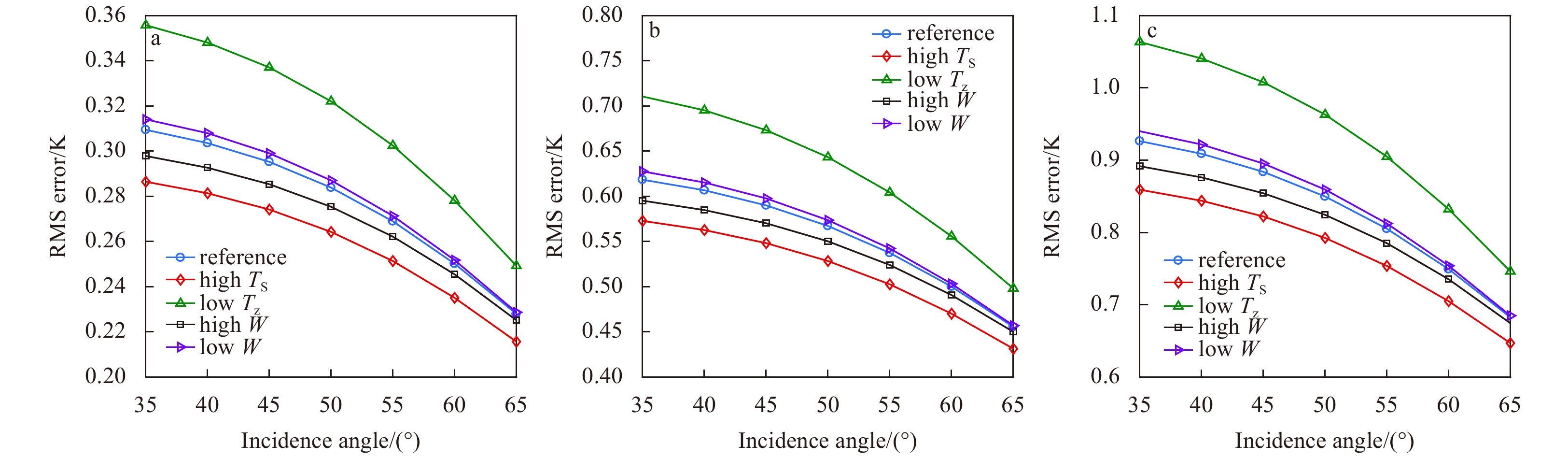
Figure 2 shows the RMS error of retrieved sea surface temperature (TS) at different incidence angles under different calibration accuracies. It can be observed that the greatest error on retrieved sea surface temperature is obtained at low TS, while the smallest error on retrieved sea surface temperature is obtained at high TS, resulting from the low sensitivity of TB to TS at low TS. For example, the RMS error of retrieved sea surface temperature under the calibration accuracy of 0.25 K is 0.302 5, 0.269 0, and 0.251 4 K when TS is 283, 293, and 303 K, respectively, for the incidence angle of 55°.
Figure
2.
The variation of RMS error of retrieved sea surface temperature with the forward model, for various levels of noise. a. Approximately 0.25 K, b. approximately 0.50 K, and c. approximately 0.75 K on TB, with the incidence angle under five homogeneous scenes (Table 2).
From Fig. 2, it can also be observed that the RMS error on retrieved sea surface temperature decreases at the edge of the swath that covers the larger incidence angles, the reason for which is that the sensitivity of TB to TS is greater at larger incidence angles. In all three configurations, with the increasing of noise on TB, the RMS error of retrieved sea surface temperature increases gradually. For instance, the error in the noise of 0.75 K (0.647 0–1.063 7 K) is greater than in the noise of 0.25 K (0.215 7–0.355 8 K).
4.2.2
Influence of the noise of auxiliary parameters on retrieved results
In the previous sections, we examined the corresponding statistics of the retrievals without auxiliary parameter errors. However, it is unrealistic to assume that auxiliary parameters perfectly known. Consequently, we tested the statistical behavior of the retrievals in different retrieval condition configurations, which are shown in Table 4. Errors on auxiliary parameters are assumed to follow a Gaussian distribution with the standard deviation ${\sigma _{{P_i}}}$. The second column of Table 4 is the priori estimate of the sea surface temperature Ts, which is 286.7 K, this value is based on Nation Centers for Environment Prediction (NCEP) Climate Forecast System Reanalysis sea surface temperature data in 2015 which is 6-hourly Products at 1.0 degree horizontal resolution. The third column of Table 4 is the standard deviation of the statistical results, which is 11.9 K. In the rest of this section, we present the results obtained with the forward model for the calibration accuracy of 0.50 K on TB measured. The calibration accuracy of 0.25 K and 0.75 K have also been examined, and the results follow the same trends as those of 0.50 K
Table
4.
Retrieval conditions tested over the five homogeneous scenes
Retrieval conditions
Prior values Pi
Uncertainties ${\sigma _{{P_i}}}$
Noise on auxiliary parameters
Nominal
${P_{ {T_{\rm S}} } } = $286.7 K
${\sigma _{ {T_{\rm S}} } } = $11.9 K
${\sigma _W} =$0.5 m·s–1, ${\sigma_{\varphi}} = $20°, ${\sigma_V} =$0.5 mm, ${\sigma_L} = $0.01 mm
$W$ perfectly/poorly known
nominal
nominal
${\sigma _W} = $0 m·s–1/1.0 m·s–1 all other $\sigma $: nominal
$\varphi $ perfectly/poorly known
nominal
nominal
${\sigma_{\varphi}} =$0°/40°, all other $\sigma $: nominal
$V$ perfectly/poorly known
nominal
nominal
${\sigma_V} =$0 mm/1.0 mm, all other $\sigma $: nominal
$L$ perfectly/poorly known
nominal
nominal
${\sigma _L} =$0 mm/0.02 mm, all other $\sigma $: nominal
Table 5 gives the RMS errors of retrieved ${T_{\rm{S}}}$ for the reference scene specified in Table 2 under the retrieval configurations in Table 4. The smallest error (0.630 6 K at incidence angle of 35° and 0.484 6 K at incidence angle of 65°) on retrieved sea surface temperature is obtained for perfectly known $W$, while the greatest error is observed for poorly known $W$. This means that the error of wind speed has the greatest influence on the retrieval of sea surface temperature. By contrast, the retrieved ${T_{\rm{S}}}$ error is only weakly sensitive to the $\varphi $, $V$, and $L$ error because the sensitivity of ${T_{\rm{B}}}$ to $\varphi $, $V$, and $L$ is lower than to $W$ for the reference scene.
Table
5.
The RMS errors of sea surface temperature retrieval for the reference scene specified in Table 2 under the retrieval configurations (Table 4)
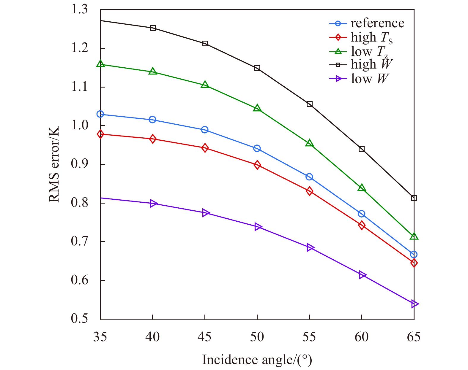
Figure 3 presents the RMS error of retrieved sea surface temperature over the five homogeneous scenes under nominal retrieval conditions. The greatest error (1.271 8 K at the incidence angle of 35° and 0.813 5 K at the incidence angle of 65°) on retrieved sea surface temperature is obtained at high W, and the error of retrieved sea surface temperature is greater than that in the case of no auxiliary parameter errors, shown in Fig. 2b; this result emphasizes the large dependence of the retrieved ${T_{\rm{S}}}$ error to the errors on auxiliary parameters.
Figure
3.
The RMS error of retrieved sea surface temperature at different incidence angles over the five homogeneous scenes under nominal retrieval conditions (Table 4).
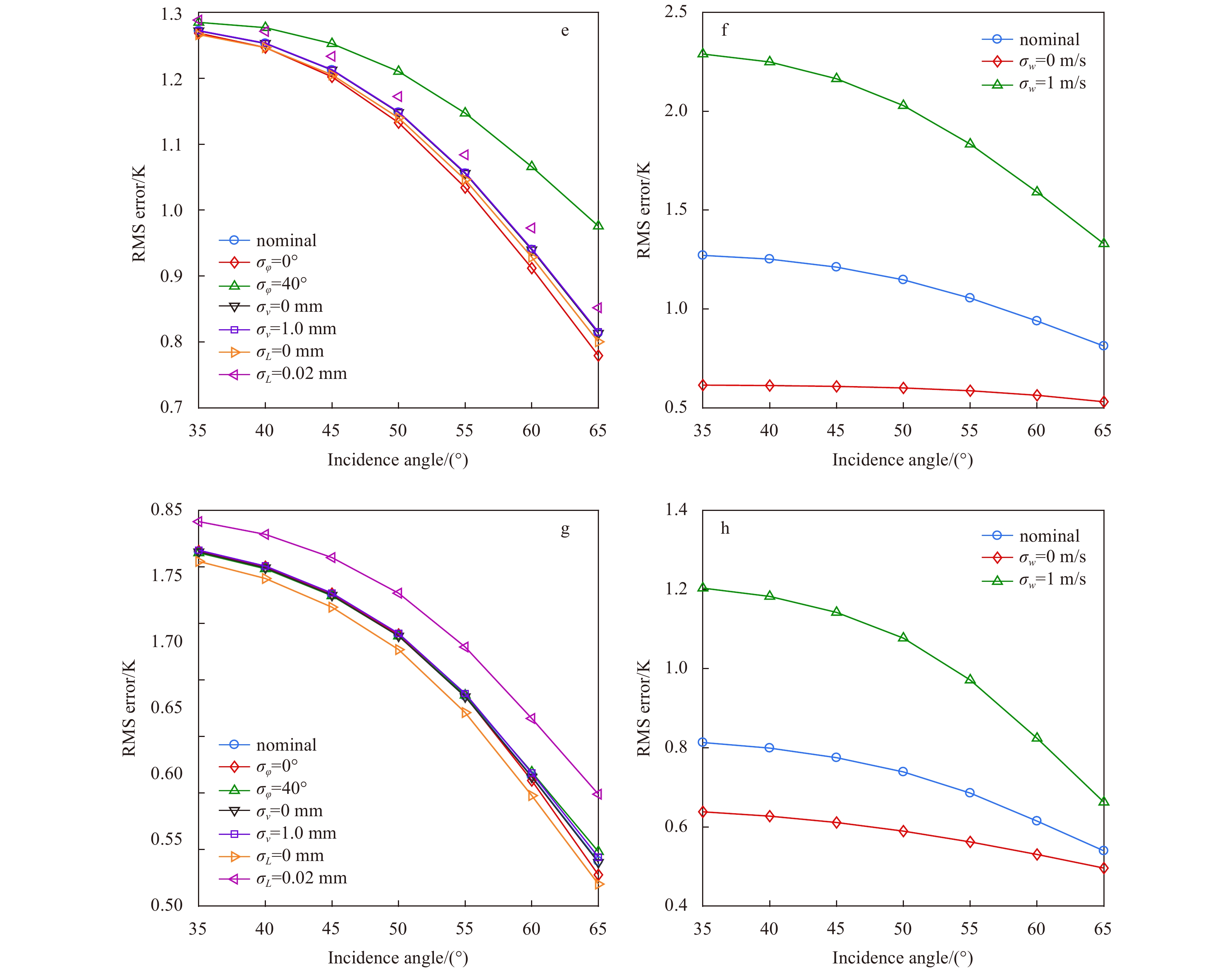
Figures 4a and b show the retrieved sea surface temperature errors obtained in the high ${T_{\rm{S}}}$ condition. It is clear that the greatest error of retrieved sea surface temperature is obtained at the wind speed error of 1.0 m/s (1.669 2 K at the incidence angle of 35°), resulting from the high sensitivity of ${T_{\rm{B}}}$ to $W$ at high ${T_{\rm{S}}}$, which will cause a large brightness temperature error. It is interesting to note that the retrieved sea surface temperature errors in the case of poorly known $L$ are slightly greater than those obtained in the conditions of poorly known $\varphi $ and $V$, but the errors are far less than those of the condition of poorly known $W$. In the conditions of the low ${T_{\rm{S}}}$ scene shown in Figs 4c and d, the results follow the same trends as those of a high ${T_{\rm{S}}}$ scene. The greatest error of retrieved ${T_{\rm{S}}}$ is also obtained at the wind speed error of 1.0 m/s, which is approximately 1.957 6 K at the incidence angle of 35°. Compared with the condition of high ${T_{\rm{S}}}$ scene, the greatest error obtained at the wind speed error of 1.0 m/s is significantly increased at the low ${T_{\rm{S}}}$ scene, due to the lower ${T_{\rm{B}}}$ sensitivity to ${T_{\rm{S}}}$ at lower ${T_{\rm{S}}}$.The errors on retrieved sea surface temperature range from 1.330 5 K at 65° to 2.289 3 K at 35° in poorly known $W$ under the high $W$ scene (Fig. 4f), and the reason is that there is greater ${T_{\rm{B}}}$ sensitivity to $W$ at higher $W$. In comparison with the scene of high and low ${T_{\rm{S}}}$, the errors of retrieved ${T_{\rm{S}}}$ in poorly known $W$ have a remarkable increase for the high $W$ scene. It should be noted that the retrieved sea surface temperature errors in the case of poorly known $\varphi $ are slightly greater than those obtained in the conditions of poorly known $V$ and $L$ for the high $W$ scene (Fig. 4e), which is different from the high and low ${T_{\rm{S}}}$ scene. Figures 4g and h show the statistics of the low $W$ scene, in which the results follow the same trends as those of the high and low ${T_{\rm{S}}}$ scene, but the errors of retrieved sea surface temperature are the smallest over all four retrieval configurations.
Figure
4.
The RMS error on retrieved sea surface temperature at different incidence angles over the high TS scene (a, b), the low TS scene (c, d), the high W scene (e, f), and the low W scene (g, h), under different retrieval conditions.
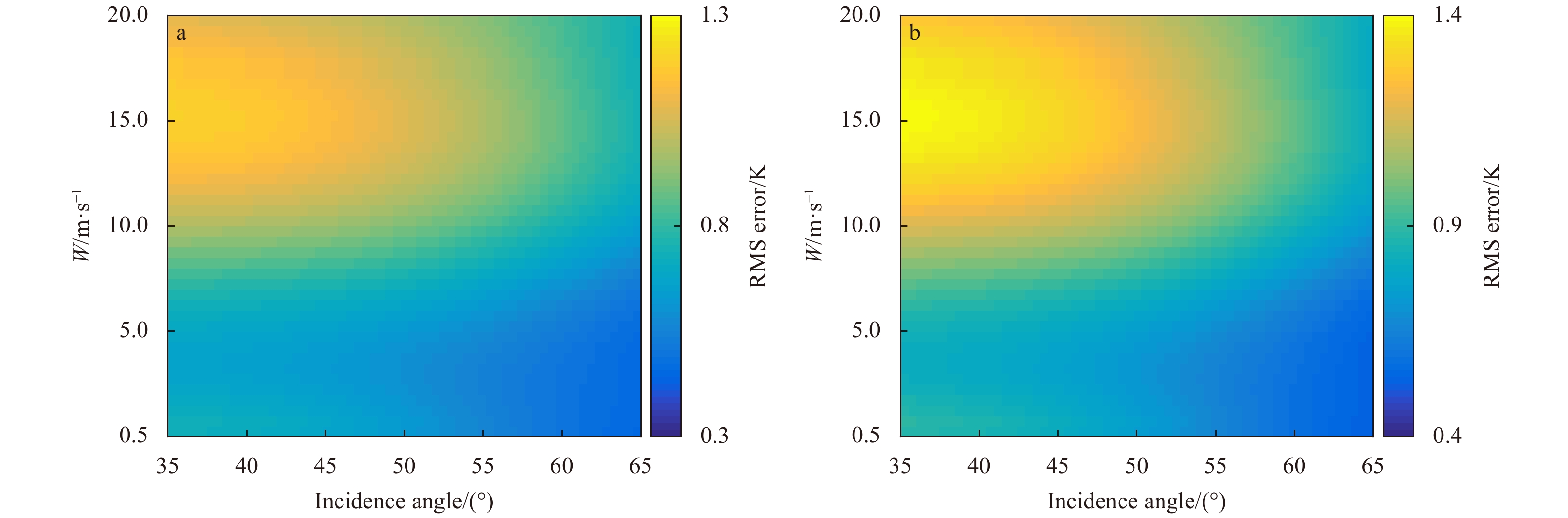
Figure 5a show the RMS errors of retrieved sea surface temperature obtained in the high ${T_{\rm{S}}}$ condition (Table 2) under nominal retrieval conditions (Table 4). It is clear that the greatest error of retrieved sea surface temperature is obtained at the wind speed of 15 m/s (1.197 9 K at the incidence angle of 35°), and the minimal error of retrieved sea surface temperature is obtained at the wind speed of 0.5 m/s (0.456 1 K at the incidence angle of 65°). We can observe that the larger the incidence angle, the more accurate the result on retrieved sea surface temperature when the wind speed is constant. When the incidence angle is constant, and the wind speed ranges from 0.5 m/s to 15 m/s, the smaller the wind speed, the more accurate the retrieved result, but there is the opposite result occurs when the wind speed ranges from 15 m/s to 20 m/s. Figure 5b show the RMS error of retrieved sea surface temperature obtained in the low ${T_{\rm{S}}}$ condition (Table 2) under nominal retrieval conditions (Table 4), the results follow the same trends as those of a high ${T_{\rm{S}}}$ scene, but the error obtained is significantly increased at the low ${T_{\rm{S}}}$ scene, due to the lower ${T_{\rm{B}}}$ sensitivity to TS at lower ${T_{\rm{S}}}$.
Figure
5.
The RMS error on retrieved sea surface temperature at different incidence angles and wind speed over the high TS scene (a), and the low TS scene (b) under nominal retrieval conditions (Table 4).
In this paper, a one-dimensional synthetic aperture microwave radiometer prototype, 1D-SAMR, is described to improve the spatial resolution of remote sensing of sea surface temperature. A radiometer detection frequency (with dual polarimetric mode) of 6.9 GHz was adopted, which is sensitive to sea surface temperature. We considered the configurations foreseen for 1D-SAMR are that the satellite orbital height is 900 km, the antenna plane is tilted by approximately 30°, and the incidence angles of 1D-SAMR on the ground range from 35° to 65°. For the 1D-SAMR instrument, the angular resolution of 0.43° can be obtained by theoretical calculation. The parabolic cylindrical antenna has a size of 12 m×10 m, and the spatial resolution along the swath is approximately 5 km.
In order to evaluate the surface temperature retrieval accuracy of 1D-SAMR, a set of idealized experiments of sea surface temperature retrieval was carried out based on the 1D-SAMR prototype, using an iterative retrieval approach. We studied two factors that affect the accuracy of sea surface temperature retrieval, including the radiometer calibration accuracy and the auxiliary geophysical parameters precision. In the case of no auxiliary parameter errors, it can be observed that the greatest error on retrieved sea surface temperature is obtained at low ${T_{\rm{S}}}$ (i.e., the RMS error is 0.710 6 K for the incidence angle of 35° under the radiometer calibration accuracy of 0.5 K), while the smallest error on retrieved sea surface temperature is obtained at high ${T_{\rm{S}}}$, due to the higher sensitivity of ${T_{\rm{B}}}$ to ${T_{\rm{S}}}$ at high ${T_{\rm{S}}}$. In addition, it can also be observed that the RMS error on retrieved sea surface temperature decreases with the incidence angle increase and the calibration accuracy improve. In the more realistic case, errors on auxiliary parameters are assumed to follow a Gaussian distribution. It is concluded that there is a large dependence of the retrieved ${T_{\rm{S}}}$ error on the errors on auxiliary parameters, and wind speed is the main sea surface signal contaminating the sea surface temperature retrieval. The greatest error on retrieved sea surface temperature was 2.289 3 K at an incidence angle of 35° in poorly known $W$ (i.e., the error on W is 1.0 m/s) over the high $W$ scene for the radiometer calibration accuracy of 0.5 K. However, the dependence of the retrieved ${T_{\rm{S}}}$ error to the errors on $\varphi $, $V$, and $L$ is very weak.
Therefore, in order to obtain high spatial resolution and high precision sea surface temperature data, it is necessary to improve the calibration accuracy of one-dimensional synthetic aperture microwave radiometers better than 0.5 K. In addition, it is necessary to improve the precision of auxiliary geophysical parameters, especially to ensure that the error of $W$ is less than 0.5 m/s.
Chelton D B, Wentz F J. 2005. Global microwave satellite observations of sea surface temperature for numerical weather prediction and climate research. Bulletin of the American Meteorological Society, 86(8): 1097–1116. doi: 10.1175/BAMS-86-8-1097
[2]
Corbella I, Duffo N, Vall-Llossera M, et al. 2004. The visibility function in interferometric aperture synthesis radiometry. IEEE Transactions on Geoscience & Remote Sensing, 42(8): 1677–1682
[3]
Curry J A, Bentamy A, Bourassa M A, et al. 2004. Seaflux. Bulletin of the American Meteorological Society, 85(3): 409–424. doi: 10.1175/BAMS-85-3-409
[4]
Font J, Camps A, Borges A, et al. 2010. SMOS: The challenging sea surface salinity measurement from space. Proceedings of the IEEE, 98(5): 649–665. doi: 10.1109/JPROC.2009.2033096
[5]
Guan L, Kawamura H. 2003. SST availabilities of satellite infrared and microwave measurements. Journal of Oceanography, 59(2): 201–209. doi: 10.1023/A:1025543305658
[6]
Kerr Y H, Waldteufel P, Wigneron J P, et al. 2001. Soil moisture retrieval from space: the Soil Moisture and Ocean Salinity (SMOS) mission. IEEE Transactions on Geoscience & Remote Sensing, 39(8): 1729–1735
[7]
Le Vine D M. 1990. The sensitivity of synthetic aperture radiometers for remote sensing applications from space. Radio Science, 25(4): 441–453. doi: 10.1029/RS025i004p00441
[8]
Le Vine D M, Griffis A J, Swift C T, et al. 1994. ESTAR: a synthetic aperture microwave radiometer for remote sensing applications. Proceedings of the IEEE, 82(12): 1787–1801. doi: 10.1109/5.338071
[9]
Le Vine D M, Kao M, Swift C T, et al. 1990. Initial results in the development of a synthetic aperture microwave radiometer. IEEE Transactions on Geoscience & Remote Sensing, 28(4): 614–619
[10]
Le Vine D M, Swift C T, Haken M. 2001. Development of the synthetic aperture microwave radiometer, ESTAR. IEEE Transactions on Geoscience & Remote Sensing, 39(1): 199–202
[11]
Liebe H J, Rosenkranz P W, Hufford G A. 1992. Atmospheric 60-GHz oxygen spectrum: New laboratory measurements and line parameters. Journal of Quantitative Spectroscopy & Radiative Transfer, 48(5–6): 629–643
[12]
Lim B H. 2009. The design and development of a geostationary synthetic thinned aperture radiometer [dissertation]. Michigan: The University of Michigan
[13]
Mätzler C. 2006. Thermal Microwave Radiation: Applications for Remote Sensing. London: Institution of Engineering & Technology
[14]
Meissner T, Wentz F J. 2004. The complex dielectric constant of pure and sea water from microwave satellite observations. IEEE Transactions on Geoscience & Remote Sensing, 42(9): 1836–1849
[15]
Meissner T, Wentz F J. 2012. The Emissivity of the ocean surface between 6 and 90 GHz over a large range of wind speeds and earth incidence angles. IEEE Transactions on Geoscience & Remote Sensing, 50(8): 3004–3026
[16]
Reynolds R W, Rayner N A, Smith T M, et al. 2002. An improved in situ and satellite SST analysis for climate. Journal of Climate, 15(13): 1609–1625. doi: 10.1175/1520-0442(2002)015<1609:AIISAS>2.0.CO;2
[17]
Rosenkranz P W. 1999. Correction [to “Water vapor microwave continuum absorption: A comparison of measurements and models” by Philip W. Rosenkranz]. Radio Science, 34(4): 1025
[18]
Ruf C S, Swift C T, Tanner A B, et al. 1988. Interferometric synthetic aperture microwave radiometry for the remote sensing of the earth. IEEE Transactions on Geoscience & Remote Sensing, 26(5): 597–611
[19]
Schanda E. 1979. Multiple wavelength aperture synthesis for passive sensing of the earth’s surface. In: Antennas and Propagation Society International Symposium. Seattle, WA, USA: IEEE, 762–763
[20]
Schwartz M J. 1998. Observation and modeling of atmospheric oxygen millimeter-wave transmittance [dissertation]. Cambridge, MA: Massachusetts Institute of Technology
[21]
Ulaby F T, Moore R K, Fung A K. 1981. Microwave Remote Sensing: Active and Passive. Volume 1: Microwave Remote Sensing Fundamentals and Radiometry. Reading, MA, USA: Addison-Wesley
[22]
Wentz F J, Meissner T. 2000. Algorithm theoretical basis document (ATBD). Version 2: AMSR ocean algorithm. Santa Rosa, CA: Remote Sensing Systems
[23]
Wentz F J, Meissner T. 2016. Atmospheric absorption model for dry air and water vapor at microwave frequencies below 100 GHz derived from spaceborne radiometer observations. Radio Science, 51(5): 381–391. doi: 10.1002/2015RS005858
[24]
Zine S, Boutin J, Font J, et al. 2008. Overview of the SMOS sea surface salinity prototype processor. IEEE Transactions on Geoscience & Remote Sensing, 46(3): 621–645
Haofeng Dou, Chengwang Xiao, Hao Li, et al. Deep Learning Imaging for 1-D Aperture Synthesis Radiometers. IEEE Transactions on Geoscience and Remote Sensing, 2023, 61: 1. doi:10.1109/TGRS.2023.3249239
2.
Chaogang Guo, Weihua Ai, Maohong Liu, et al. Sea surface temperature retrieval based on simulated space-borne one-dimensional multifrequency synthetic aperture microwave radiometry. Frontiers in Environmental Science, 2022, 10 doi:10.3389/fenvs.2022.1054076
3.
Guangmin Sun, Pan Ma, Jie Liu, et al. Design and Implementation of a Novel Interferometric Microwave Radiometer for Human Body Temperature Measurement. Sensors, 2021, 21(5): 1619. doi:10.3390/s21051619
Figure 1. Diagram of the iterative process to retrieve sea surface temperature.
Figure 2. The variation of RMS error of retrieved sea surface temperature with the forward model, for various levels of noise. a. Approximately 0.25 K, b. approximately 0.50 K, and c. approximately 0.75 K on TB, with the incidence angle under five homogeneous scenes (Table 2).
Figure 3. The RMS error of retrieved sea surface temperature at different incidence angles over the five homogeneous scenes under nominal retrieval conditions (Table 4).
Figure 4. The RMS error on retrieved sea surface temperature at different incidence angles over the high TS scene (a, b), the low TS scene (c, d), the high W scene (e, f), and the low W scene (g, h), under different retrieval conditions.
Figure 5. The RMS error on retrieved sea surface temperature at different incidence angles and wind speed over the high TS scene (a), and the low TS scene (b) under nominal retrieval conditions (Table 4).


 DownLoad:


 DownLoad: