Peilong Yu, Lifeng Zhang, Mingyang Liu, Quanjia Zhong, Yongchui Zhang, Xin Li. A comparison of the strength and position variability of the Kuroshio Extension SST front[J]. Acta Oceanologica Sinica, 2020, 39(5): 26-34. doi: 10.1007/s13131-020-1567-3
Citation:
Peilong Yu, Lifeng Zhang, Mingyang Liu, Quanjia Zhong, Yongchui Zhang, Xin Li. A comparison of the strength and position variability of the Kuroshio Extension SST front[J]. Acta Oceanologica Sinica, 2020, 39(5): 26-34. doi: 10.1007/s13131-020-1567-3
Peilong Yu, Lifeng Zhang, Mingyang Liu, Quanjia Zhong, Yongchui Zhang, Xin Li. A comparison of the strength and position variability of the Kuroshio Extension SST front[J]. Acta Oceanologica Sinica, 2020, 39(5): 26-34. doi: 10.1007/s13131-020-1567-3
Citation:
Peilong Yu, Lifeng Zhang, Mingyang Liu, Quanjia Zhong, Yongchui Zhang, Xin Li. A comparison of the strength and position variability of the Kuroshio Extension SST front[J]. Acta Oceanologica Sinica, 2020, 39(5): 26-34. doi: 10.1007/s13131-020-1567-3
College of Meteorology and Oceanography, National University of Defense Technology, Nanjing 211101, China
2.
No. 91939 Troops of PLA, Jiangmen 529100, China
3.
State Key Laboratory of Numerical Modeling for Atmospheric Sciences and Geophysical Fluid Dynamics (LASG), Institute of Atmospheric Physic, Chinese Academy of Sciences, Beijing 100029, China
4.
College of Earth Science, University of Chinese Academy of Sciences, Beijing 100049, China
Funds:
The National Natural Science Foundation of China under contract Nos 41975066, 41605051 and 41406003; the Open Research Fund of State Key Laboratory of Estuarine and Coastal Research under contract No. SKLEC-KF201707; the High-Tech Innovation Think-Tank Youth Project under contract No. DXB-ZKQN-2016-019; Jiangsu Provincial Natural Science Foundation under contract No. BK20130064.
This study compares the seasonal and interannual-to-decadal variability in the strength and position of the Kuroshio Extension front (KEF) using high-resolution satellite-derived sea surface temperature (SST) and sea surface height (SSH) data. Results show that the KEF strength has an obvious seasonal variation that is similar at different longitudes, with a stronger (weaker) KEF during the cold (warm) season. However, the seasonal variation in the KEF position is relatively weak and varies with longitude. In contrast, the low-frequency variation of the KEF position is more distinct than that of the KEF strength even though they are well correlated. On both seasonal and interannual-to-decadal time scales, the western part of the KEF (142°–144°E) has the greatest variability in strength, while the eastern part of the KEF (149°–155°E) has the greatest variability in position. In addition, the relationships between wind-forced Rossby waves and the low-frequency variability in the KEF strength and position are also discussed by using the statistical analysis methods and a wind-driven hindcast model. A positive (negative) North Pacific Oscillation (NPO)-like atmospheric forcing generates positive (negative) SSH anomalies over the central North Pacific. These oceanic signals then propagate westward as Rossby waves, reaching the KE region about three years later, favoring a strengthened (weakened) and northward (southward)-moving KEF.
After separating from the east coast of Japan near 35°N, the Kuroshio in the open North Pacific is known as the Kuroshio Extension (KE), characterized by large-amplitude meanders and energetic pinch-off eddies (Mizuno and White, 1983; Qiu and Chen, 2005; Kelly et al., 2010). Numerous studies have demonstrated that the KE system exhibits pronounced decadal variations between stable and unstable states (e.g., Qiu and Chen, 2005, 2010; Taguchi et al., 2007). In its stable state, the KE jet is strengthened and shifts northward, with weakened regional eddy activity and an intensified southern recirculation gyre. The opposite situation occurs in the unstable state. Previous studies have indicated that the transition between the two dynamic states is triggered mainly by the arrival of wind-forced Rossby waves that form in the central North Pacific (e.g., Qiu, 2003; Qiu and Chen, 2005, 2010; Sasaki et al., 2013; Qiu et al., 2014).
The warm KE converges with the cold Oyashio current in the north, which strengthens the climatological meridional gradient in sea surface temperature (SST), forming a subarctic frontal zone (SAFZ). However, the SAFZ is not single and has two major SST fronts (Yasuda, 2003; Nonaka et al., 2006; Seo et al., 2014; Kida et al., 2015). One is the subarctic front along the Oyashio Extension and the other is associated with the KE system and is known as the KE front (KEF). The two fronts have different vertical structure and may also be governed by different mechanisms (Nonaka et al., 2006). Therefore, studies focusing on the KEF are essential for a better understanding of the SAFZ.
The KEF is also recognized as a region with vigorous air–sea interaction. In winter, the turbulent heat release is enhanced over the warmer flank of the KEF, which induces strong surface wind convergence and thus leads to local maxima of cloudiness (Tokinaga et al., 2009; Masunaga et al., 2015, 2016). In early summer, the stronger vertical mixing over the warmer flank of the KEF results in a higher low-level cloud base than that over its cooler flank (Kawai et al., 2015). Moreover, during this season the KEF contributes to the eastward extension of the Baiu rainband through surface wind convergence (Tokinaga et al., 2009). These findings indicate that the impacts of the KEF on the overlying atmosphere can penetrate into the free troposphere. Other studies have also identified the significant impact of SST anomalies along the KEF on the large-scale atmospheric circulation (e.g., Frankignoul et al., 2011; O’Reilly and Czaja, 2015). Accordingly, the KEF is also significant for studies of North Pacific air–sea interaction and climate.
The availability of high-resolution SST data after the 1980s facilitates the investigation of KEF variability. Chen (2008) explored the variations in the KEF strength and position on seasonal and longer time scales. Wang et al. (2016) further investigated the seasonal and interannual-to-decadal variability in the KEF position both temporally and spatially, but did not discuss the variability in the KEF strength. The similarities and differences between the variability in the KEF strength and position remain poorly understood. Moreover, some studies have indicated that the low-frequency KEF meridional shift is modulated mainly by oceanic Rossby waves (Chen, 2008; Seo et al., 2014). However, whether the low-frequency variability in the KEF strength is also controlled by oceanic Rossby waves remains unknown. The interannual-to-decadal relationship between the KEF strength and position variability is also unclear. To address these questions, the present paper aims to compare the variability in the KEF strength with that of the KEF position on seasonal and longer time scales, both temporally and spatially, using a high-resolution satellite-derived SST dataset on a 0.25° × 0.25° grid (Reynolds et al., 2007). In addition, the relationships between wind-forced Rossby waves and the low-frequency variability in the KEF strength and position are also discussed.
The remainder of this paper is organized as follows. Section 2 introduces the dataset and method, and Section 3 investigates the seasonal and interannual-to-decadal variability in the KEF strength and position. A discussion of the results and the conclusions are given in Section 4 and Section 5, respectively.
2.
Data and method
We used the monthly SST field from the National Oceanic and Atmospheric Administration (NOAA) optimum interpolation SST product (OISST), which is based on Advanced Very High Resolution Radiometer (AVHRR) infrared satellite data (Reynolds et al., 2007). This SST dataset has a high spatial resolution of 0.25° and was used in the period from January 1993 to December 2015. The monthly sea surface height (SSH) anomaly field was derived from the Archiving, Validation, and Interpretation of Satellite Oceanographic (AVISO) altimeter satellite product (Ducet et al., 2000) with a spatial resolution of 0.25° that covers the period from January 1993 to December 2015. We also used the monthly sea level pressure (SLP) and surface wind stress fields obtained from the National Centers of Environmental Prediction–National Center for Atmospheric Research (NCEP–NCAR) reanalysis dataset (Kalnay et al., 1996) on a 2.5° × 2.5° grid from January 1993 to December 2015.
The horizontal SST gradient $\left| {\nabla T} \right|$ was calculated following Chen (2008):
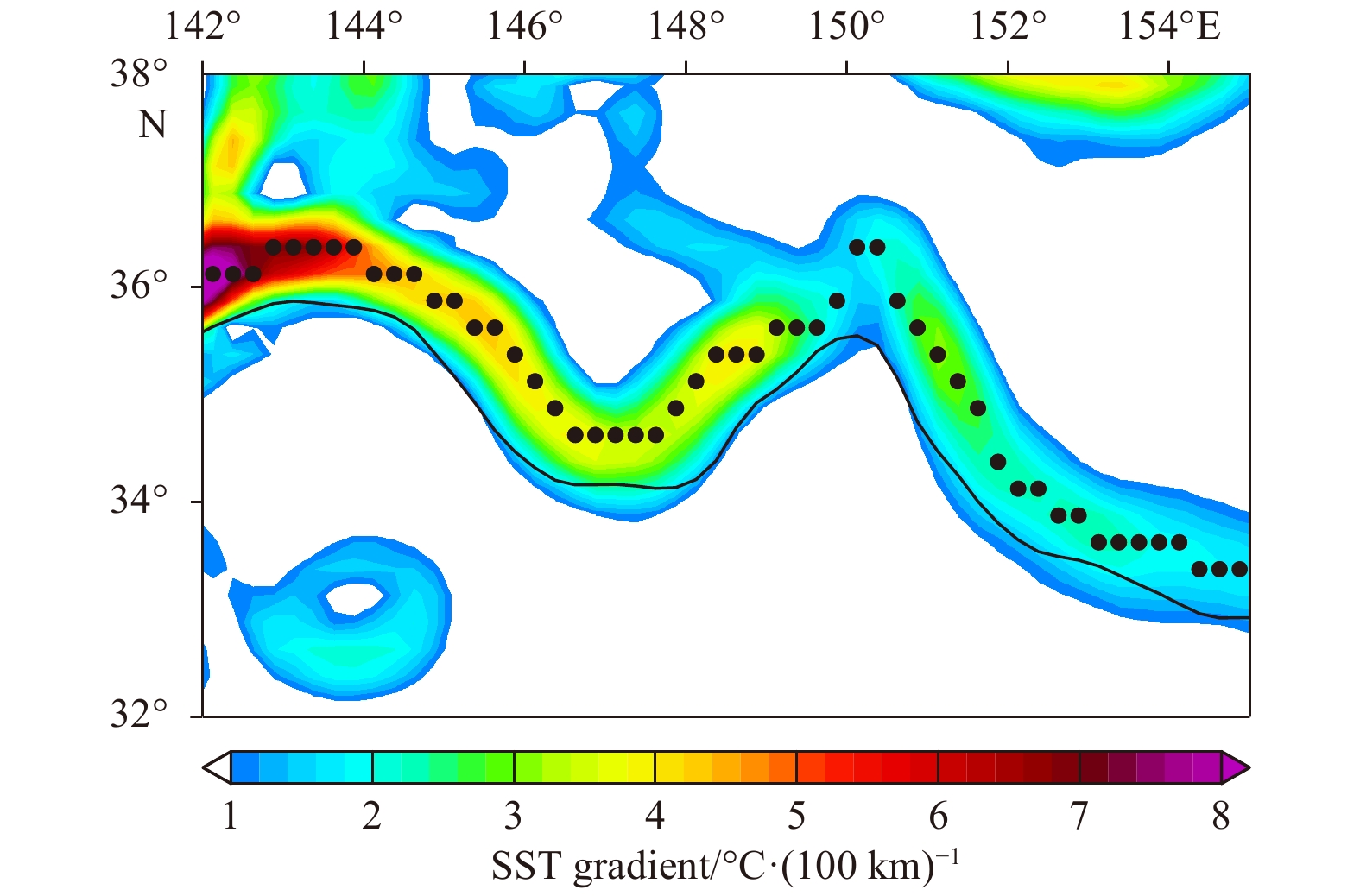
where T is SST and $\left({x,y} \right)$ are the zonal and meridional coordinates, respectively. Then, following Seo et al. (2014), we searched for the KEF position defined as the latitude of the maximum $\left| {\nabla T} \right|$ between 31.875° and 37.625°N at each longitudinal grid point from 142° to 155°E for each calendar month. However, this method may confuse the mesoscale eddies and the subarctic front, which also have large SST gradients, with the KEF. To solve this problem, we slightly modified the search process of KEF proposed by Seo et al. (2014) and attempted to identify the KEF by detecting the KE jet axis. Specifically, at each longitude between 142° and 155°E, we searched the latitude of the maximum $\left| {\nabla T} \right|$ whose distance to the KE jet axis is less than or equal to 200 km and defined it as the KEF position (Fig. 1). This method is based on the fact that the KEF is adjacent to the KE jet axis (Chen, 2008; Seo et al., 2014). Thus, the erroneous grid points associated with the subarctic front can be excluded by this modified procedure. According to Sugimoto et al. (2014), here a continuous 110-cm SSH contour from 142° to 155°E was used as the KE jet axis, which can remove the influence of an eddy with a closed contour. The $\left| {\nabla T} \right|$ at the KEF position denotes the KEF strength.
Figure
1.
The horizontal SST gradient $\left| {\nabla T} \right|$ in December 2008. The black dots represent the KEF position estimated from the modified search process of Seo et al. (2014). The thick black line indicates the KE jet axis, which is defined as the 110 cm SSH contour.
In this study, the 13-month running mean filter, which is often believed to reduce the components whose periods are shorter than one year effectively, was used to exclude the seasonal signals in the data. Considering this filter may also retain some seasonal changes (Esbensen, 1984), we still used another method to remove the seasonal cycle by subtracting the monthly climatology. It can be seen that this method can also effectively remove the seasonal changes in the time series (Fig. 5). In the following sections, the results derived from the 13-month running mean filter are primarily shown because those derived by subtracting the monthly climatology are virtually the same.
Figure
5.
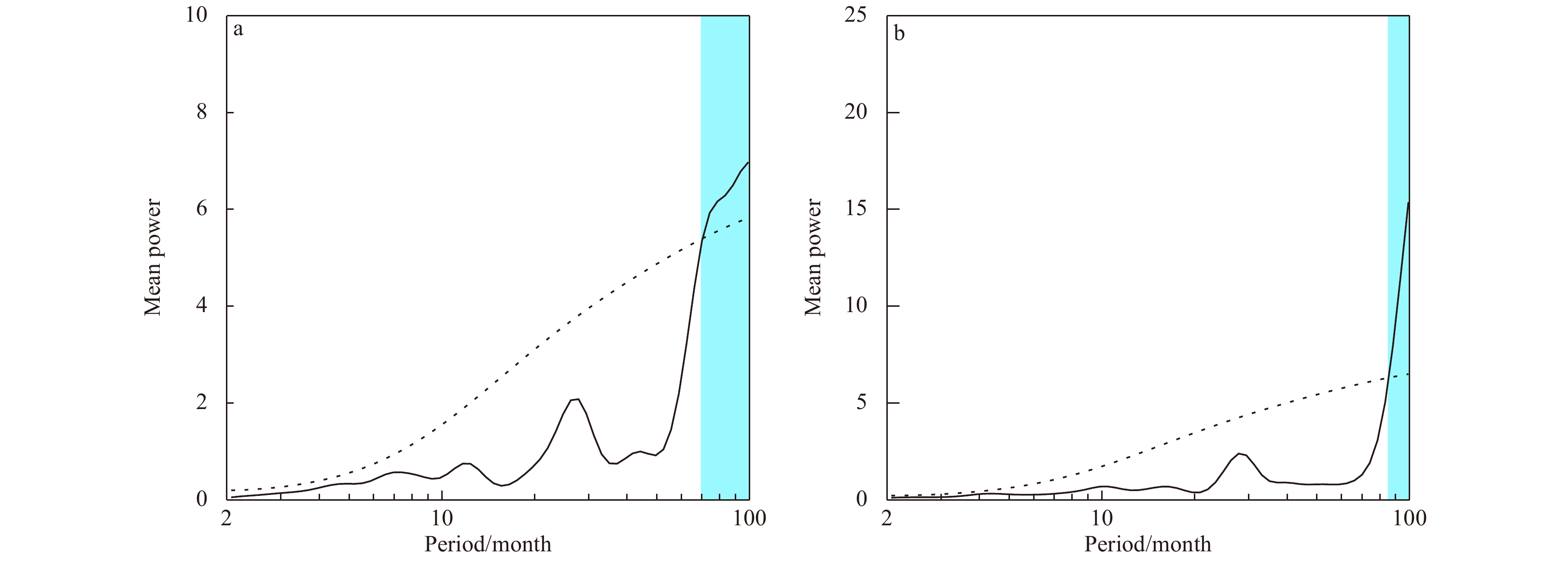
Global wavelet power spectra of the normalized time series of the overall mean KEF strength (a) and position (b). The dotted lines designate the 90% confidence levels against red noise. The shaded bars represent bands with significant periods. To highlight the low-frequency variability, the seasonal cycle in the time series of the KEF strength and position was removed before the calculation of the wavelet power spectrum, by subtracting the monthly climatology.
Linear correlation and regression analysis were also performed, and their statistical significance was estimated by a two-tailed Student’s t-test using the effective number of degrees of freedom (Bretherton et al., 1999; Ding et al., 2015; Zheng et al., 2015, 2016), which considers serial-autocorrelation.
3.
Results
3.1
Seasonal variability in the KEF strength and position
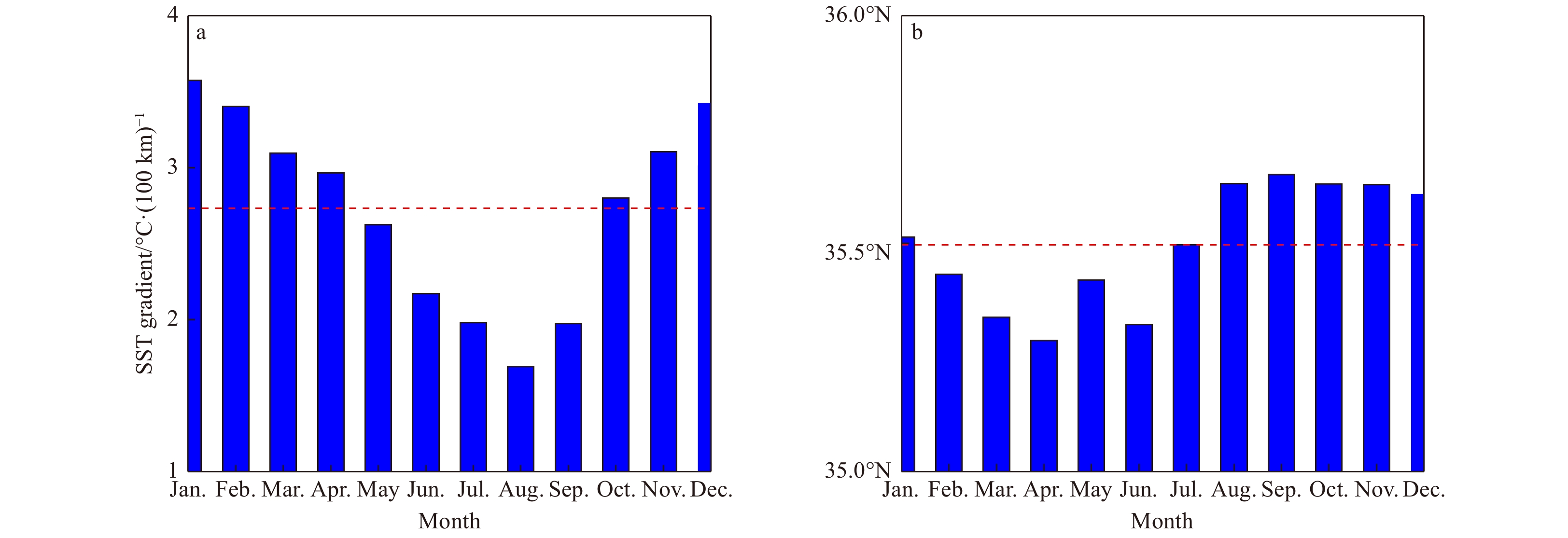
Averaged over the band 142°–155°E, the overall mean KEF strength shows an obvious seasonal variation. As shown in Fig. 2a, the KEF strength peaks in January and weakens gradually after that, reaching a minimum in August. The seasonal variation in the KEF position is quite different from that of the KEF strength. The KEF is farthest north in September and farthest south in April (Fig. 2b); however, the difference between these two positions is only 0.36° in latitude, indicating that the seasonal variation of the KEF position is weak.
Figure
2.
Seasonal variation in the KEF strength (a) and position (b) averaged over the band 142°–155°E. The red dashed lines denote the annual mean of KEF strength and position.
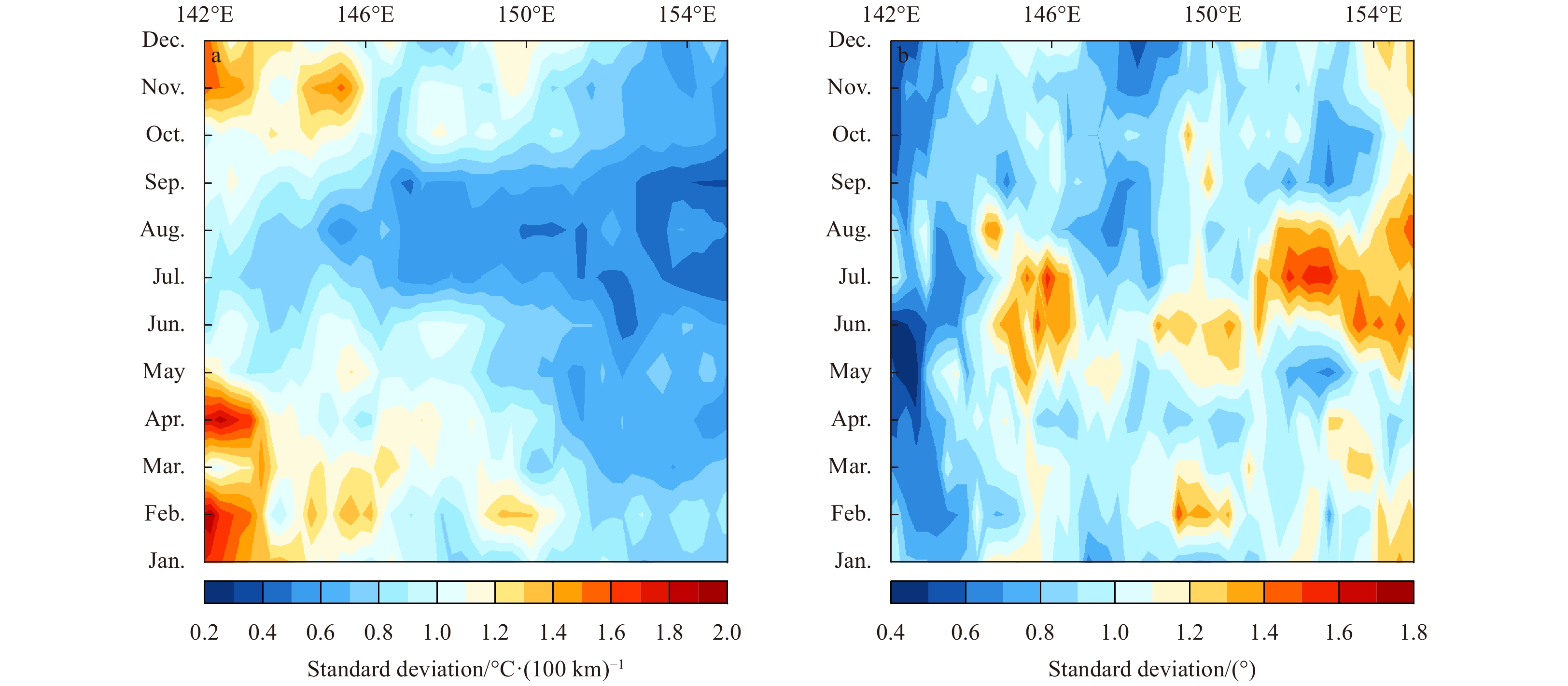
The spatial distribution of seasonal variations in the KEF strength and position is further investigated. As shown in Fig. 3a, in each calendar month the KEF strength has almost the same longitudinal distribution, which reaches a maximum around 142°E and weakens with increasing longitude. The KEF strength at different longitudes also shows similar seasonal variation to that of the averaged strength in Fig. 2a, with a stronger KEF during the cold season (November–April) and a weaker KEF during the warm season (June–September). In contrast, the KEF position has different seasonal variations at different longitudes (Fig. 3b). In each calendar month, the KEF position in the bands 142°–145°E and 148°–151°E is farther north than at other longitudes. The KEF position is farther south in August than in other months from 142° to 145°E, while from 148° to 151°E the KEF position is farther south in February than in other months. The seasonal variation in the KEF position is also different in other longitudinal bands. From 145° to 148°E, the KEF position is farther north in November than in other months, but it is farther north in September than in other months from 151° to 155°E. We also measured the amplitudes (defined as one standard deviation of the KEF strength and position in each calendar month) of the seasonal variations in the KEF strength and position between 142° and 155°E. The seasonal variation in the KEF strength is most evident over 142°–144°E, and weakens with increasing longitude (Fig. 3c); however, the seasonal variation in the KEF position is stronger to the east of 151°E than 142°–144°E and shows a maximum around 148.5°E (Fig. 3d).
Figure
3.
Seasonal variations in the KEF strength (a) and position (b) at each longitude between 142°E and 155°E,and the seasonal variation amplitude of the KEF strength (C) and the KEF position (d) estimated as one standard deviation in each calendar month.
3.2
Interannual-to-decadal variability in the KEF strength and position
Figure 4a shows a time series of the KEF strength averaged from 142° to 155°E. The data show obvious low-frequency variations that can exceed 3.7°C/(100 km) on interannual and longer time scales. Specifically, the overall mean KEF strength weakens in 1993–1997, intensifies in 1997–2004, weakens again in 2004–2006, returns to a strong state in 2006–2011, and drops to a weak state in 2011–2013, and then has an increasing trend after 2013. Low-frequency variations are also clear in the time series of the KEF position averaged from 142° to 155°E (Fig. 3b), which shows a north–south movement that can exceed 2° in latitude. After applying the 13-month running mean filter, the KEF strength time series has a significant positive correlation of r = 0.67 with the position time series. Similar results can also be derived by subtracting the monthly climatology (r = 0.61). This indicates a northward (southward) migration of the KEF when it becomes strong (weak). Previous studies have reported the strong simultaneous correlation between the low-frequency variations of KE jet strength and position (Qiu and Chen, 2005, 2010; Sugimoto et al., 2014). These works support our finding set out above because the KEF variations closely follow the behavior of the KE jet (Chen, 2008).
Figure
4.
Time series of the KEF strength (a) and position (b) averaged over 142°–155°E. The red lines denote the 13-month running mean. The gray lines indicate the mean values over 1981–2015.
Wavelet analysis further reveals that the low-frequency variations in the KEF strength and position have significant periods of longer than 6 (Fig. 5a) and 7 years (Fig. 5b), respectively. These results indicate that both the KEF strength and position have pronounced interannual and decadal variations. Figure 5 also shows that the mean power of the pronounced period of the position time series is clearly stronger than that of the strength time series. This indicates that the KEF position has more distinct low-frequency variations than the KEF strength.
Figure 6a shows the interannual standard deviation of the KEF strength at each longitude between 142° and 155°E in each calendar month. Over the whole year, the low-frequency variability in the KEF strength generally decreases with longitude. The standard deviation of the KEF position near the bands 142°–144°E and 146°–149°E is smaller than that at other longitudes throughout the year (Fig. 6b). In particular, the minimum standard deviation appears between 142° and 144°E. In contrast, the maximum standard deviation of the KEF position exists to the east of 149°E. This longitudinal distribution of the low-frequency variability is similar to that of the seasonal variability in the KEF strength and position ( Figs 3c, d).
Figure
6.
Interannual standard deviation of the KEF strength (a) and position (b) at each longitude between 142° and 155°E in each calendar month.
Considering that the low-frequency variability in both the KEF strength and position varies with longitude, we also divided the KEF (142°–155°E) into three parts: the western part of the KEF (KEFw, 142°–144°E), the central part of the KEF (KEFc, 144°–149°E), and the eastern part of the KEF (KEFe, 149°–155°E). Figure 6 shows that the low-frequency variability in the KEF strength (position) is strongest over the KEFw (KEFe). Note that compared with the other parts of the KEF, the KEFw (KEFe) also has stronger seasonal variability in the KEF strength (position) (Figs 3c, d). Furthermore, the wavelet power spectra of the monthly time series of the KEF strength and position in different parts were calculated (not shown). For the KEF strength, the KEFc shows significant period of longer than 6 years, as for the overall mean KEF (Fig. 5a). However, there are no significant periods in either spectrum of the KEFw and KEFe. For the KEF position, significant low-frequency variability is mainly reflected in the KEFc and KEFe.
3.3
Comparison with previous studies
The seasonal and interannual-to-decadal variability in the KEF strength and position revealed in the present study is generally consistent with that reported by Chen (2008) and Wang et al. (2016). Nevertheless, our results also show some differences with these previous studies. For instance, Wang et al. (2016) reported that at longitudes other than 142°–145°E and 148°–151°E, the KEF position has a similar seasonal variability. However, we found that the seasonal variability in the KEF position is also different at other longitudinal bands (Fig. 3b). This discrepancy may be attributed to the differences in the methods used to detect the KEF. In our work, we modified the method of Seo et al. (2014) and searched for the location of the maximum whose distance to the KE jet axis is less than or equal to 200 km and defined it as the KEF position. In contrast, Wang et al. (2016) used the KE jet axis as the initial KEF position and adjusted it toward the local maximum of the SST gradient and applied a three-point running mean to update the KEF position. Repeating this procedure five times, the final KEF position was obtained. Therefore, the KEF detected by Wang et al. (2016) was spatially smoother than that in the present study, which may explain the slight discrepancy. Note that the study region here is also different from those used by Wang et al. (2016). We used the region 31.875°–37.625°N, 142°–155°E, while Wang et al. (2016) used the region 30°–40°N, 141°–158°E. However, when we used the same study region as that employed by Wang et al. (2016), there are still some differences between the two studies and our results are similar to those obtained using our original region. For this reason, the differences in the study region between the present study and Wang et al. (2016) are not believed to be the key factors contributing to the differences in the KEF variability and its longitudinal distribution.
4.
Discussion
Chen (2008) indicated that the low-frequency KEF variability is closely related to changes in the KE dynamic states. Previous studies suggested that the wind-forced Rossby waves are the main drivers of changes in the KE dynamic state (see introduction and references therein). Accordingly, the low-frequency KEF variability is thought to be strongly impacted by oceanic Rossby waves. A close relationship between low-frequency KEF position variability and oceanic Rossby waves has been identified (Chen, 2008; Seo et al., 2014). According to the results of Section 3.2, the low-frequency KEF strength and position variability are linked simultaneously, so the former should also be controlled by oceanic Rossby waves. To test the above hypotheses, the relationships between wind-forced Rossby waves and the low-frequency variability in the KEF strength and position were discussed in this section.
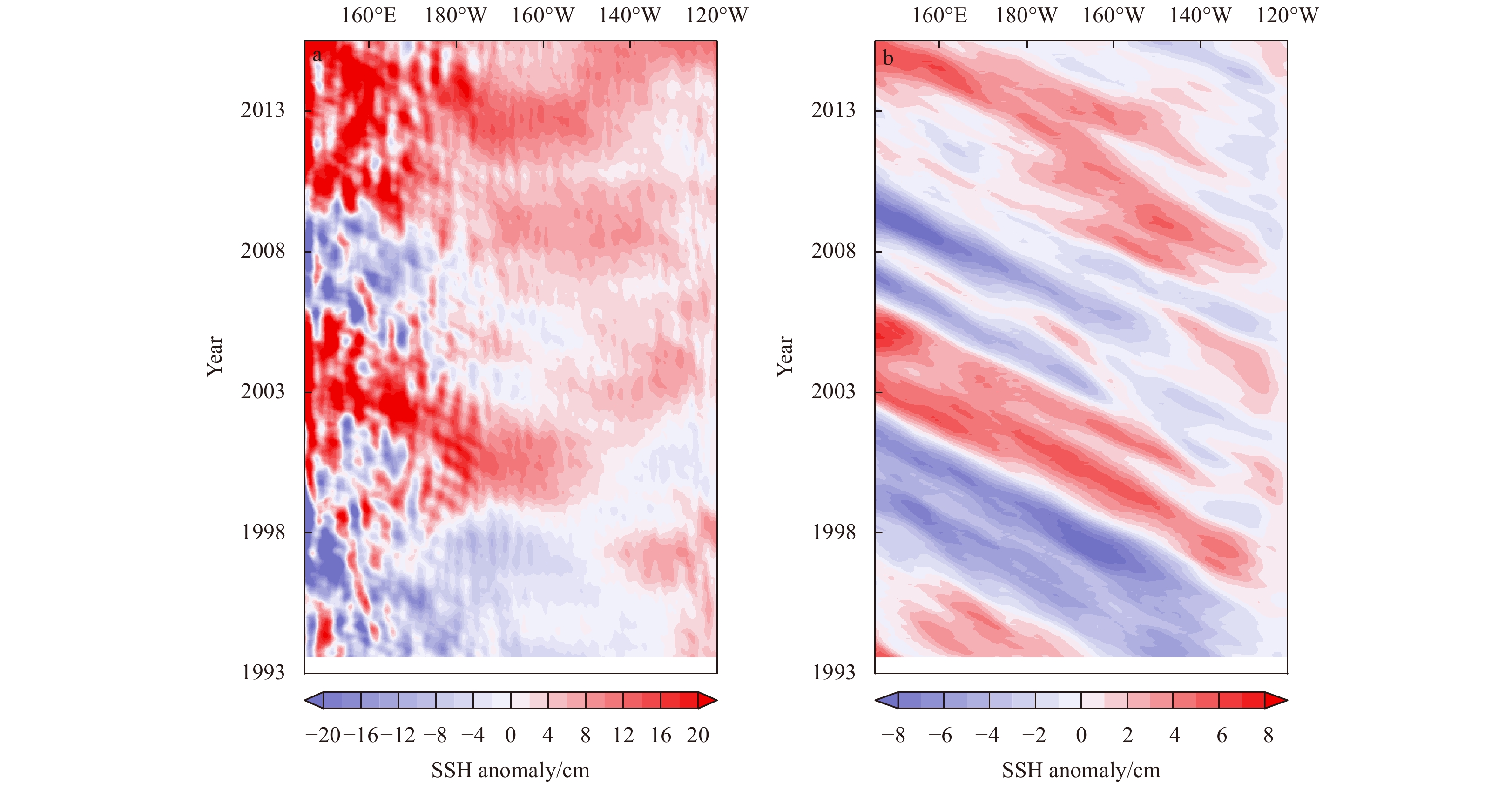
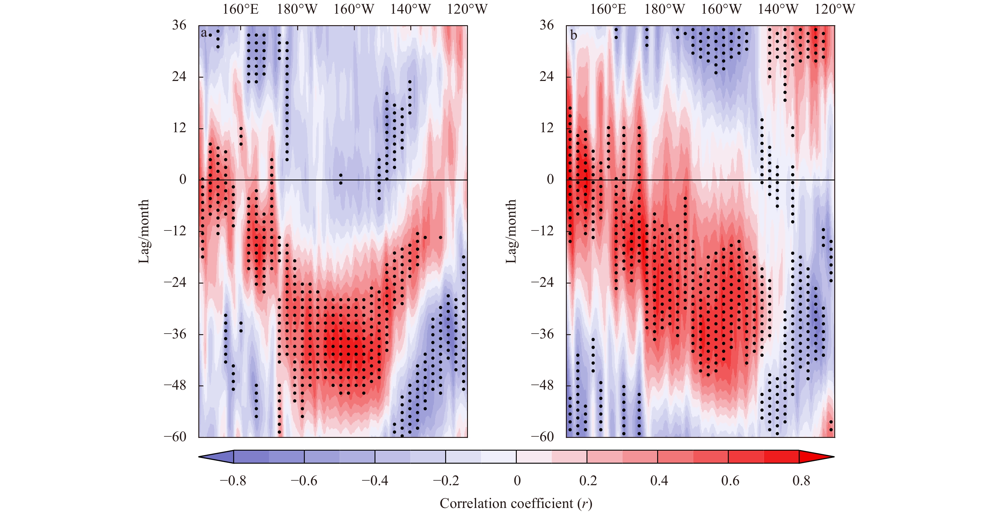
Figure 7a shows the SSH anomalies averaged over the 33°–35°N band, where the zonal mean KE axis is located (Seo et al., 2014). It is clear that low-frequency SSH variations in the central North Pacific propagate westward into the KE region, featuring the oceanic Rossby waves. Based on this observation, we examined the relationships between oceanic Rossby waves and the low-frequency variability in the KEF strength and position. As shown in Fig. 8b, the KEF position variation has significant positive correlations with the SSH anomalies formed in the central North Pacific around 170°W at a lead time of 36 months (3 years). These oceanic signals associated with the KEF meridional shift propagate westward into the KE region at a lead time of 0 year, indicating that the low-frequency KEF position variability is modulated by oceanic Rossby waves. These results are consistent with the findings of Chen (2008) and Seo et al. (2014). Similarly, the low-frequency KEF strength variation is synchronous with the arrival of oceanic Rossby waves into the KE region (Fig. 8a), suggesting that the changes in the KEF strength are also impacted by oceanic Rossby waves. Because the positive (negative) SSH anomalies are consistent with the deepening (shoaling) of main thermocline depth that results in the formation of positive (negative) SST anomalies (Sugimoto and Hanawa, 2011; Seo et al., 2014), the close relationships between oceanic Rossby waves and the low-frequency variations in the KEF strength and position can be explained as follows. When the positive (negative) SSH anomalies propagate westward into the KE region as oceanic Rossby waves, they lead to the convergence (divergence) of warm water and thus strengthen (weaken) the SST gradient to the north (Chen, 2008). This finally causes a strengthened (weakened) and northward (southward)-moving KEF.
Figure
7.
Time–longitude diagram of 13-month running mean SSH anomalies averaged over the 33°–35°N band from the AVISO satellite data (a) and the wind-driven baroclinic Rossby wave model (b).
Figure
8.
Lag–longitude correlation diagram of the 13-month running mean KEF strength time series (a) and the KEF position time series (b) with the SSH anomalies. Positive lags mean that the KEF strength leads the SSH anomalies. The stippled areas indicate statistical significance above the 90% confidence level.
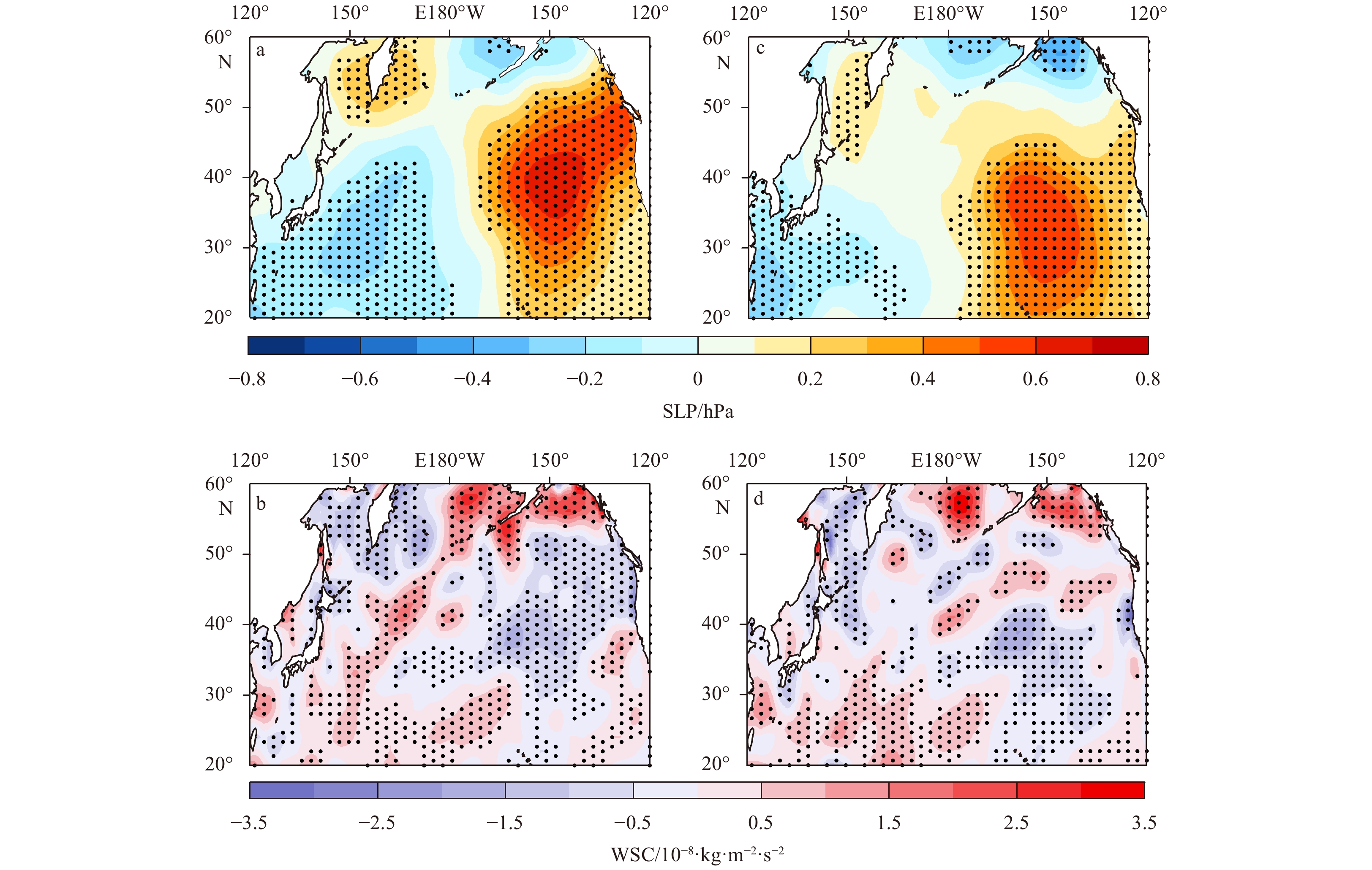
In addition, previous studies have shown that oceanic Rossby waves are excited mainly by atmospheric fluctuations in the central North Pacific (e.g., Qiu, 2003; Qiu and Chen, 2005; Kwon and Deser, 2007; Taguchi et al., 2007; Ceballos et al., 2009; Sasaki et al., 2013). Therefore, we have also investigated the relationships between these atmospheric fluctuations and the low-frequency variations in the KEF strength and position. In the three years before the northward (southward) shift of the KEF, the atmospheric fluctuations show a meridional dipole pattern over the central and eastern North Pacific, characterized by negative (positive) SLP anomalies in the north and positive (negative) SLP anomalies in the south (Fig. 9c). This atmospheric dipole structure is similar to the positive (negative) phase of the North Pacific Oscillation (NPO; Wallace and Gutzler, 1981; Linkin and Nigam, 2008), which is associated with a northward (southward) shift of the Aleutian Low (Sugimoto and Hanawa, 2009; Yu et al., 2016, 2017). The positive (negative) SLP anomalies in the south of the NPO-like dipole are accompanied by negative (positive) surface wind stress curl (WSC) over the central North Pacific (Fig. 9d), which can generate the positive (negative) SSH anomalies through Ekman convergence (divergence). These results indicate that the NPO-like atmospheric forcing is responsible for the excitation of oceanic Rossby waves, which is consistent with previous findings (Sugimoto and Hanawa, 2009; Sasaki et al., 2013; Seo et al., 2014). We also found that the KEF intensity change is significantly related to a similar atmospheric dipole pattern over the central and eastern North Pacific with a lead of 3 years (Figs 9a, b).
Figure
9.
Regressions of the SLP (a) and WSC (b) anomalies onto the normalized KEF strength time series with a lag of 36 months. The time series of SLP and KEF strength are smoothed by a 13-month running mean filter. The stippled areas indicate statistical significance exceeding the 90% confidence level. Figure c, d are the same as a, b, but for the normalized KEF position time series after smoothing by a 13-month running mean filter, respectively.
From the above, a positive NPO-like atmospheric dipole, which is associated with a northward shift in the Aleutian Low, generates the positive SSH anomalies over the central North Pacific through Ekman convergence. These oceanic signals then propagate westward as Rossby waves, reaching the KE region and resulting in the convergence of warm water, which tends to strengthen the KEF and displace this oceanic front northward. To further verify these results, we adopted a simple baroclinic Rossby wave model. Specifically, under the long-wave approximation, the linear vorticity equation is
where h is the SSH anomaly, ${c_R}$ is the speed of the long baroclinic Rossby waves, g is the gravitational constant, g′ is the reduced gravity, ${\rho _0}$ is the reference density of seawater, f is the Coriolis parameter, and τ is the curl of anomalous wind stress vector. The solution of Eq. (2) can be obtained by integrating this equation along the baroclinic Rossby wave characteristic:
Given the WSC data, we can easily hindcast the $h\left({x,t} \right)$ field from Eq. (3). It should be noted that in Eq. (3), the solution due to the eastern boundary forcing at $x = 0$ has been ignored according to Fu and Qiu (2002). Similar to Fig. 7a, Fig. 7b shows the time–longitude diagram of the modeled SSH anomalies over the same latitudinal band. It is found that the hindcast low-frequency SSH changes from the Rossby wave model well correspond to those from the observation over the KE region in the west of 155°E. The correlation coefficient between the observed and modeled SSH anomalies can reach r = 0.62, which exceeds the 90% confidence level, indicating a good hindcast skill of the linear Rossby wave model.
Based on this wind-driven baroclinic Rossby wave model, the relationships among the NPO-like atmospheric forcing, oceanic Rossby waves and the KEF variations were re-examined. Firstly, the WSC forcing is obtained by projecting the NPO-like pattern in Fig. 9d onto the NCEP–NCAR WSC anomalies in each month. Similar results can also be obtained when the NPO-like pattern in Fig. 9c was adopted. Then, using this WSC forcing, we hindcast the SSH anomalies again based on Eq. (3).
It is found that the modeled SSH anomalies averaged over the KE region from the NPO-like atmospheric forcing has significant correlations of r = 0.43 and r = 0.47 with the KEF intensity change and meridional shift, respectively. These results support that the oceanic Rossby waves excited by the NPO-like atmospheric forcing significantly modulate the low-frequency variations in the KEF strength and position.
5.
Conclusions
With the aid of high-resolution satellite-derived SST and SSH data, the seasonal and interannual-to-decadal variability in the KEF strength and position were compared in the present study. The overall mean KEF strength has an obvious seasonal variation, with the strongest KEF in January and the weakest KEF in August. However, the seasonal variations in the KEF position are relatively weak. On interannual and decadal time scales, variations are evident in the KEF strength and position. The changes in the KEF strength can exceed 3.7°C/(100 km) and have significant period of longer than 6 years. The KEF position shows a north–south movement that can exceed 2° of latitude, with significant period of longer than 7 years. The low-frequency KEF strength and position variations are well correlated. Nevertheless, the KEF position has more distinct low-frequency variations than the KEF strength. Spatially, the KEF strength shows similar seasonal variations at different longitudes to its overall mean, with a stronger KEF during the cold season and a weaker KEF during the warm season. In contrast, the seasonal variations in the KEF position are different over the different longitudinal bands. Both the seasonal and low-frequency variability in the KEF strength are strongest over the western part of the KEF (142°–144°E), while those of the KEF position are strongest over the eastern part of the KEF (149°–155°E).
The relationships between wind-forced Rossby waves and the low-frequency variability in the KEF strength and position were also discussed by using the statistical analysis methods and a wind-driven hindcast model. A positive (negative) NPO-like atmospheric forcing generates positive (negative) SSH anomalies over the central North Pacific. These oceanic signals then propagate westwards as Rossby waves, reaching the KE region about three years later, leading to a strengthened (weakened) and northward (southward)-moving KEF. However, the reasons for the seasonal variations in the KEF strength and position remain unclear. Chen (2008) inferred that the relevant mechanisms may be related to surface heat flux forcing; this possibility also deserves further investigation.
Bretherton C S, Widmann M, Dymnikov V P, et al. 1999. The effective number of spatial degrees of freedom of a time-varying field. Journal of Climate, 12(7): 1990–2009. doi: 10.1175/1520-0442(1999)012<1990:TENOSD>2.0.CO;2
[2]
Ceballos L I, Di Lorenzo E, Hoyos C D, et al. 2009. North Pacific Gyre Oscillation synchronizes climate fluctuations in the eastern and western boundary systems. Journal of Climate, 22(19): 5163–5174. doi: 10.1175/2009JCLI2848.1
[3]
Chen Shuiming. 2008. The Kuroshio Extension front from satellite sea surface temperature measurements. Journal of Oceanography, 64(6): 891–897. doi: 10.1007/s10872-008-0073-6
[4]
Ding Ruiqiang, Li Jianping, Tseng Y H. 2015. The impact of South Pacific extratropical forcing on ENSO and comparisons with the North Pacific. Climate Dynamics, 44(7–8): 2017–2034. doi: 10.1007/s00382-014-2303-5
[5]
Ducet N, Le Traon P Y, Reverdin G. 2000. Global high-resolution mapping of ocean circulation from TOPEX/Poseidon and ERS-1 and -2. Journal of Geophysics Research: Oceans, 105(C8): 19477–19498. doi: 10.1029/2000JC900063
[6]
Esbensen S K. 1984. A comparison of intermonthly and interannual teleconnections in the 700 mb geopotential height field during the northern hemisphere winter. Monthly Weather Review, 112(10): 2016–2032. doi: 10.1175/1520-0493(1984)112<2016:ACOIAI>2.0.CO;2
[7]
Frankignoul C, Sennéchael N, Kwon Y O, et al. 2011. Influence of the meridional shifts of the Kuroshio and the Oyashio Extensions on the atmospheric circulation. Journal of Climate, 24(3): 762–777. doi: 10.1175/2010JCLI3731.1
[8]
Fu L L, Qiu Bo. 2002. Low-frequency variability of the North Pacific Ocean: the roles of boundary-and wind-driven baroclinic Rossby waves. Journal of Geophysics Research: Oceans, 107(C12): 13-1–13-10. doi: 10.1029/2001JC001131
[9]
Kalnay E, Kanamitsu M, Kistler R, et al. 1996. The NCEP-NCAR 40-Year reanalysis project. Bulletin of the American Meteorological Society, 77(3): 437–472. doi: 10.1175/1520-0477(1996)077<0437:TNYRP>2.0.CO;2
[10]
Kawai Y, Miyama T, Iizuka S, et al. 2015. Marine atmospheric boundary layer and low-level cloud responses to the Kuroshio Extension front in the early summer of 2012: three-vessel simultaneous observations and numerical simulations. Journal of Oceanography, 71(5): 511–526. doi: 10.1007/s10872-014-0266-0
[11]
Kelly K A, Small R J, Samelson R M, et al. 2010. Western boundary currents and frontal air-sea interaction: Gulf Stream and Kuroshio Extension. Journal of Climate, 23(21): 5644–5667. doi: 10.1175/2010JCLI3346.1
[12]
Kida S, Mitsudera H, Aoki S, et al. 2015. Oceanic fronts and jets around Japan: a review. Journal of Oceanography, 71(5): 469–497. doi: 10.1007/s10872-015-0283-7
[13]
Kwon Y O, Deser C. 2007. North Pacific decadal variability in the Community Climate System Model version 2. Journal of Climate, 20(11): 2416–2433. doi: 10.1175/JCLI4103.1
[14]
Linkin M E, Nigam S. 2008. The North Pacific Oscillation-west Pacific teleconnection pattern: mature-phase structure and winter impacts. Journal of Climate, 21(9): 1979–1997. doi: 10.1175/2007JCLI2048.1
[15]
Masunaga R, Nakamura H, Miyasaka T, et al. 2015. Separation of climatological imprints of the Kuroshio Extension and Oyashio fronts on the wintertime atmospheric boundary layer: Their sensitivity to SST resolution prescribed for atmospheric reanalysis. Journal of Climate, 28(5): 1764–1787. doi: 10.1175/JCLI-D-14-00314.1
[16]
Masunaga R, Nakamura H, Miyasaka T, et al. 2016. Interannual modulations of oceanic imprints on the wintertime atmospheric boundary layer under the changing dynamical regimes of the Kuroshio Extension. Journal of Climate, 29(9): 3273–3296. doi: 10.1175/JCLI-D-15-0545.1
[17]
Mizuno K, White W B. 1983. Annual and interannual variability in the Kuroshio current system. Journal of Physical Oceanography, 13(10): 1847–1867. doi: 10.1175/1520-0485(1983)013<1847:AAIVIT>2.0.CO;2
[18]
Nonaka M, Nakamura H, Tanimoto Y, et al. 2006. Decadal variability in the Kuroshio-Oyashio Extension simulated in an eddy-resolving OGCM. Journal of Climate, 19(10): 1970–1989. doi: 10.1175/JCLI3793.1
[19]
O’Reilly C H, Czaja A. 2015. The response of the Pacific storm track and atmospheric circulation to Kuroshio Extension variability. Quarterly Journal of the Royal Meteorological Society, 141(686): 52–66. doi: 10.1002/qj.2334
[20]
Qiu Bo. 2003. Kuroshio Extension variability and forcing of the Pacific decadal oscillations: responses and potential feedback. Journal of Physical Oceanography, 33(12): 2465–2482. doi: 10.1175/2459.1
[21]
Qiu Bo, Chen Shuiming. 2005. Variability of the Kuroshio Extension jet, recirculation gyre, and mesoscale eddies on decadal time scales. Journal of Physical Oceanography, 35(11): 2090–2103. doi: 10.1175/JPO2807.1
[22]
Qiu Bo, Chen Shuiming. 2010. Eddy-mean flow interaction in the decadally modulating Kuroshio Extension system. Deep-Sea Research Part II: Topical Studies in Oceanography, 57(13–14): 1098–1110. doi: 10.1016/j.dsr2.2008.11.036
[23]
Qiu Bo, Chen Shuiming, Schneider N, et al. 2014. A coupled decadal prediction of the dynamic state of the Kuroshio Extension system. Journal of Climate, 27(4): 1751–1764. doi: 10.1175/JCLI-D-13-00318.1
[24]
Reynolds R W, Smith T M, Liu Chunying, et al. 2007. Daily high-resolution-blended analyses for sea surface temperature. Journal of Climate, 20(22): 5473–5496. doi: 10.1175/2007JCLI1824.1
[25]
Sasaki Y N, Minobe S, Schneider N. 2013. Decadal response of the Kuroshio Extension jet to Rossby waves: Observation and thin-jet theory. Journal of Physical Oceanography, 43(2): 442–456. doi: 10.1175/JPO-D-12-096.1
[26]
Seo Y, Sugimoto S, Hanawa K. 2014. Long-term variations of the Kuroshio Extension path in winter: meridional movement and path state change. Journal of Climate, 27(15): 5929–5940. doi: 10.1175/JCLI-D-13-00641.1
[27]
Sugimoto S, Hanawa K. 2009. Decadal and interdecadal variations of the Aleutian low activity and their relation to upper oceanic variations over the North Pacific. Journal of the Meteorological Society of Japan, 87(4): 601–614. doi: 10.2151/jmsj.87.601
[28]
Sugimoto S, Hanawa K. 2011. Roles of SST anomalies on the wintertime turbulent heat fluxes in the Kuroshio-Oyashio confluence region: Influences of warm eddies detached from the Kuroshio Extension. Journal of Climate, 24(24): 6551–6561. doi: 10.1175/2011JCLI4023.1
[29]
Sugimoto S, Kobayashi N, Hanawa K. 2014. Quasi-decadal variation in intensity of the western part of the winter subarctic SST front in the western North Pacific: The influence of Kuroshio Extension path state. Journal of Physical Oceanography, 44(10): 2753–2762. doi: 10.1175/JPO-D-13-0265.1
[30]
Taguchi B, Xie Shangping, Schneider N, et al. 2007. Decadal variability of the Kuroshio Extension: observations and an eddy-resolving model hindcast. Journal of Climate, 20(11): 2357–2377. doi: 10.1175/JCLI4142.1
[31]
Tokinaga H, Tanimoto Y, Xie Shangping, et al. 2009. Ocean frontal effects on the vertical development of clouds over the western North Pacific: In situ and satellite observations. Journal of Climate, 22(16): 4241–4260. doi: 10.1175/2009JCLI2763.1
[32]
Wallace J M, Gutzler D S. 1981. Teleconnections in the geopotential height field during the Northern Hemisphere winter. Monthly Weather Review, 109(4): 784–812. doi: 10.1175/1520-0493(1981)109<0784:TITGHF>2.0.CO;2
[33]
Wang Yanxin, Yang Xiaoyi, Hu Jianyu. 2016. Position variability of the Kuroshio Extension sea surface temperature front. Acta Oceanologica Sinica, 35(7): 30–35. doi: 10.1007/s13131-016-0909-7
[34]
Yasuda I. 2003. Hydrographic structure and variability in the Kuroshio-Oyashio transition area. Journal of Oceanography, 59(4): 389–402. doi: 10.1023/A:1025580313836
[35]
Yu Peilong, Zhang Lifeng, Liu Hu, et al. 2017. A dual-period response of the Kuroshio Extension SST to Aleutian Low activity in the winter season. Acta Oceanologica Sinica, 36(9): 1–9. doi: 10.1007/s13131-017-1104-1
[36]
Yu Peilong, Zhang Lifeng, Zhang Yongchui, et al. 2016. Interdecadal change of winter SST variability in the Kuroshio Extension region and its linkage with Aleutian atmospheric low pressure system. Acta Oceanologica Sinica, 35(5): 24–37. doi: 10.1007/s13131-016-0859-0
[37]
Zheng Chongwei, Li Chongyin. 2015. Variation of the wave energy and significant wave height in the China Sea and adjacent waters. Renewable and Sustainable Energy Reviews, 43: 381–387. doi: 10.1016/j.rser.2014.11.001
[38]
Zheng Chongwei, Li Chongyin, Pan Jing, et al. 2016. An overview of global ocean wind energy resources evaluations. Renewable and Sustainable Energy Reviews, 53: 1240–1251. doi: 10.1016/j.rser.2015.09.063
Xuying Hu, Yixuan Li, Yue Dong, et al. Population characteristics of the dominant cold-water brittle star Ophiura sarsii vadicola (Ophiurida, Ophiuroidea) in the Yellow Sea. Journal of Oceanology and Limnology, 2025. doi:10.1007/s00343-024-4003-2
2.
Ting Lü, Hao Zhou, Mengfan He, et al. The summer pattern of phytoplankton pigment assemblages in response to water masses in the Yellow Sea. Journal of Oceanology and Limnology, 2025. doi:10.1007/s00343-025-4220-3
3.
Lei Zhang, Weishuai Xu, Maolin Li. Frontal slope: A new measure of ocean fronts. Journal of Sea Research, 2024, 199: 102493. doi:10.1016/j.seares.2024.102493
4.
Qi Zhang, Wenjin Sun, Huaihai Guo, et al. A Transfer Learning-Enhanced Generative Adversarial Network for Downscaling Sea Surface Height through Heterogeneous Data Fusion. Remote Sensing, 2024, 16(5): 763. doi:10.3390/rs16050763
5.
XingZe Zhang, YongHong Wang. Formation and preservation mechanisms of magnetofossils in the surface sediments of muddy areas in the yellow and Bohai Seas, China. Marine Geology, 2024, 477: 107401. doi:10.1016/j.margeo.2024.107401
6.
Zhaoyi Wang, Wei Yang, Guisheng Song, et al. Distribution, Seasonality, and Water‐Mass Transformation of Temperature and Salinity Inversions in the Southern Yellow Sea. Journal of Geophysical Research: Oceans, 2024, 129(4) doi:10.1029/2023JC020317
7.
Weishuai Xu, Lei Zhang, Xiaodong Ma, et al. The Parameterized Oceanic Front-Guided PIX2PIX Model: A Limited Data-Driven Approach to Oceanic Front Sound Speed Reconstruction. Journal of Marine Science and Engineering, 2024, 12(11): 1918. doi:10.3390/jmse12111918
8.
Yakun Xu, Xinxin Yang, Rui Xiao, et al. Long-Chain Alkenones in the South Yellow Sea Sediments and Their Indicative Significance for Haptophytes Species. Journal of Ocean University of China, 2024, 23(5): 1287. doi:10.1007/s11802-024-5970-9
9.
Hao Li, Fangguo Zhai, Yujie Dong, et al. Interannual-decadal variations in the Yellow Sea Cold Water Mass in summer during 1958–2016 using an eddy-resolving hindcast simulation based on OFES2. Continental Shelf Research, 2024, 275: 105223. doi:10.1016/j.csr.2024.105223
10.
Weishuai Xu, Lei Zhang, Ming Li, et al. Data-Driven Analysis of Ocean Fronts’ Impact on Acoustic Propagation: Process Understanding and Machine Learning Applications, Focusing on the Kuroshio Extension Front. Journal of Marine Science and Engineering, 2024, 12(11): 2010. doi:10.3390/jmse12112010
11.
Qianshuo Zhao, Huimin Huang, Mark John Costello, et al. Climate change projections show shrinking deep-water ecosystems with implications for biodiversity and aquaculture in the Northwest Pacific. Science of The Total Environment, 2023, 861: 160505. doi:10.1016/j.scitotenv.2022.160505
12.
XingZe Zhang, YongHong Wang, GuangXue Li, et al. Authigenic greigite in late MIS 3 sediments: Implications for the Yellow Sea Cold Water Mass and Yellow Sea Warm Current evolution. Marine Geology, 2023, 460: 107057. doi:10.1016/j.margeo.2023.107057
13.
Weishuai Xu, Lei Zhang, Hua Wang, et al. Spatiotemporal characterization and prediction of the subsurface temperature front of the Kuroshio extension. Journal of Sea Research, 2023, 196: 102444. doi:10.1016/j.seares.2023.102444
14.
Changyuan Chen, Chen Wang, Huimin Li, et al. Detection and characteristics analysis of the western subarctic front using the high-resolution SST product. Acta Oceanologica Sinica, 2023, 42(6): 24. doi:10.1007/s13131-022-2102-5
15.
Yichao Ren, Xianhui Men, Yu Yu, et al. Effects of transportation stress on antioxidation, immunity capacity and hypoxia tolerance of rainbow trout (Oncorhynchus mykiss). Aquaculture Reports, 2022, 22: 100940. doi:10.1016/j.aqrep.2021.100940
16.
Hui Zheng, Wen-Zhou Zhang. An extreme warm event of the Yellow Sea Cold Water Mass in the summer of 2007 and its causes. Ocean Modelling, 2022, 176: 102067. doi:10.1016/j.ocemod.2022.102067
17.
Song-yin Wang, Wei-dong Zhai. Regional differences in seasonal variation of air–sea CO2 exchange in the Yellow Sea. Continental Shelf Research, 2021, 218: 104393. doi:10.1016/j.csr.2021.104393
18.
Yibo Wang, Xiaoke Hu, Yanyu Sun, et al. Influence of the cold bottom water on taxonomic and functional composition and complexity of microbial communities in the southern Yellow Sea during the summer. Science of The Total Environment, 2021, 759: 143496. doi:10.1016/j.scitotenv.2020.143496
19.
Martin J. Head. Review of the Early–Middle Pleistocene boundary and Marine Isotope Stage 19. Progress in Earth and Planetary Science, 2021, 8(1) doi:10.1186/s40645-021-00439-2
20.
Minghan Zhu, Rujun Yang, Yan Li, et al. Seasonal and spatial variabilities of dissolved iron in southern Yellow Sea. Chemosphere, 2020, 256: 126856. doi:10.1016/j.chemosphere.2020.126856
21.
Han Su, Rujun Yang, Yan Li, et al. Influence of humic substances on iron distribution in the East China Sea. Chemosphere, 2018, 204: 450. doi:10.1016/j.chemosphere.2018.04.018
22.
Xiaoshou Liu, Qinghe Liu, Yan Zhang, et al. Effects of Yellow Sea Cold Water Mass on marine nematodes based on biological trait analysis. Marine Environmental Research, 2018, 141: 167. doi:10.1016/j.marenvres.2018.08.013
23.
S. L. Zhao, D. A. Wu. The Response of Storm Surge with Different Typhoon Tracks in Jiangsu Coastal. International Journal of Environmental Science and Development, 2017, 8(8): 570. doi:10.18178/ijesd.2017.8.8.1017
24.
Li Li, Wang Xiaojing, Liu Jihua, et al. Dissolved trace metal (Cu, Cd, Co, Ni, and Ag) distribution and Cu speciation in the southern Yellow Sea and Bohai Sea, China. Journal of Geophysical Research: Oceans, 2017, 122(2): 1190. doi:10.1002/2016JC012500
25.
Qin-Sheng Wei, Xian-Sen Li, Bao-Dong Wang, et al. Seasonally chemical hydrology and ecological responses in frontal zone of the central southern Yellow Sea. Journal of Sea Research, 2016, 112: 1. doi:10.1016/j.seares.2016.02.004
26.
Xuemei Xu, Kunpeng Zang, Cheng Huo, et al. Aragonite saturation state and dynamic mechanism in the southern Yellow Sea, China. Marine Pollution Bulletin, 2016, 109(1): 142. doi:10.1016/j.marpolbul.2016.06.009
27.
Xuemei Xu, Kunpeng Zang, Huade Zhao, et al. Monthly CO2 at A4HDYD station in a productive shallow marginal sea (Yellow Sea) with a seasonal thermocline: Controlling processes. Journal of Marine Systems, 2016, 159: 89. doi:10.1016/j.jmarsys.2016.03.009
28.
Liang Xue, Longjun Zhang, Wei-Jun Cai, et al. Air–sea CO2 fluxes in the southern Yellow Sea: An examination of the continental shelf pump hypothesis. Continental Shelf Research, 2011, 31(18): 1904. doi:10.1016/j.csr.2011.09.002
29.
Longjun Zhang, Liang Xue, Meiqin Song, et al. Distribution of the surface partial pressure of CO2 in the southern Yellow Sea and its controls. Continental Shelf Research, 2010, 30(3-4): 293. doi:10.1016/j.csr.2009.11.009
Peilong Yu, Lifeng Zhang, Mingyang Liu, Quanjia Zhong, Yongchui Zhang, Xin Li. A comparison of the strength and position variability of the Kuroshio Extension SST front[J]. Acta Oceanologica Sinica, 2020, 39(5): 26-34. doi: 10.1007/s13131-020-1567-3
Peilong Yu, Lifeng Zhang, Mingyang Liu, Quanjia Zhong, Yongchui Zhang, Xin Li. A comparison of the strength and position variability of the Kuroshio Extension SST front[J]. Acta Oceanologica Sinica, 2020, 39(5): 26-34. doi: 10.1007/s13131-020-1567-3
Figure 1. The horizontal SST gradient $\left| {\nabla T} \right|$ in December 2008. The black dots represent the KEF position estimated from the modified search process of Seo et al. (2014). The thick black line indicates the KE jet axis, which is defined as the 110 cm SSH contour.
Figure 5. Global wavelet power spectra of the normalized time series of the overall mean KEF strength (a) and position (b). The dotted lines designate the 90% confidence levels against red noise. The shaded bars represent bands with significant periods. To highlight the low-frequency variability, the seasonal cycle in the time series of the KEF strength and position was removed before the calculation of the wavelet power spectrum, by subtracting the monthly climatology.
Figure 2. Seasonal variation in the KEF strength (a) and position (b) averaged over the band 142°–155°E. The red dashed lines denote the annual mean of KEF strength and position.
Figure 3. Seasonal variations in the KEF strength (a) and position (b) at each longitude between 142°E and 155°E,and the seasonal variation amplitude of the KEF strength (C) and the KEF position (d) estimated as one standard deviation in each calendar month.
Figure 4. Time series of the KEF strength (a) and position (b) averaged over 142°–155°E. The red lines denote the 13-month running mean. The gray lines indicate the mean values over 1981–2015.
Figure 6. Interannual standard deviation of the KEF strength (a) and position (b) at each longitude between 142° and 155°E in each calendar month.
Figure 7. Time–longitude diagram of 13-month running mean SSH anomalies averaged over the 33°–35°N band from the AVISO satellite data (a) and the wind-driven baroclinic Rossby wave model (b).
Figure 8. Lag–longitude correlation diagram of the 13-month running mean KEF strength time series (a) and the KEF position time series (b) with the SSH anomalies. Positive lags mean that the KEF strength leads the SSH anomalies. The stippled areas indicate statistical significance above the 90% confidence level.
Figure 9. Regressions of the SLP (a) and WSC (b) anomalies onto the normalized KEF strength time series with a lag of 36 months. The time series of SLP and KEF strength are smoothed by a 13-month running mean filter. The stippled areas indicate statistical significance exceeding the 90% confidence level. Figure c, d are the same as a, b, but for the normalized KEF position time series after smoothing by a 13-month running mean filter, respectively.


 DownLoad:


 DownLoad: