


Figure
1.
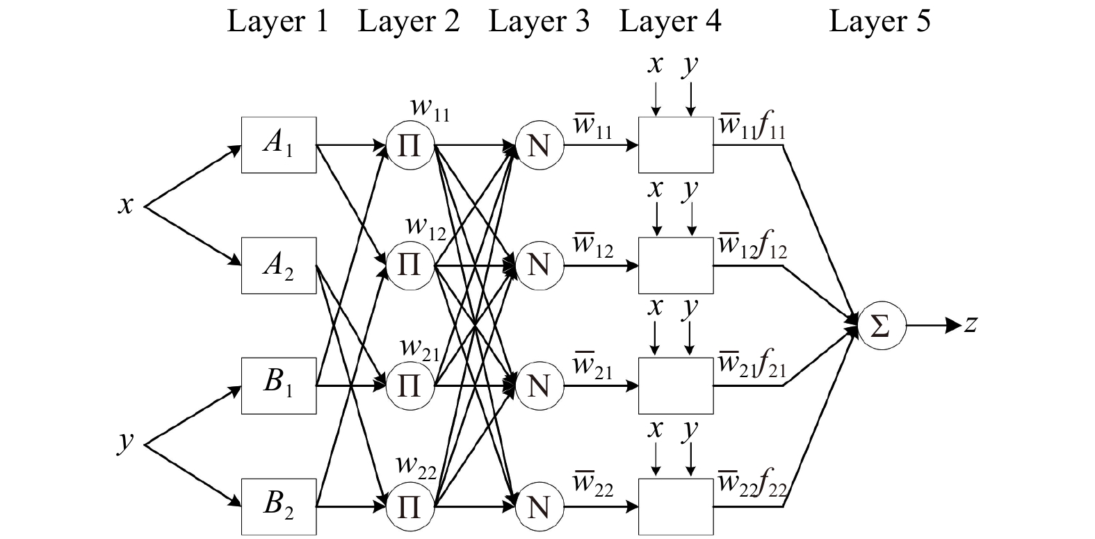
General architecture of ANFIS comprising four rules.
| Citation: | Bao Wang, Bin Wang, Wenzhou Wu, Changbai Xi, Jiechen Wang. Sea-water-level prediction via combined wavelet decomposition, neuro-fuzzy and neural networks using SLA and wind information[J]. Acta Oceanologica Sinica, 2020, 39(5): 157-167. doi: 10.1007/s13131-020-1569-1

|
Variations in sea-water level (SWL) strongly influence coastal activities and the marine navigation of vessels. Fluctuations in SWL are primarily affected by the gravitational attraction effected by the moon and sun on earth. Additionally, SWL is influenced by hydrometeorological conditions, such as low atmospheric pressure, and the occurrence of winds, typhoons, cold fronts, ocean currents, etc. The prediction and analysis of SWL variations constitute the core requirements of marine security and coastal management. Therefore, the reliable and accurate prediction of SWL is one of the major challenges faced by oceanic researchers.
Harmonic analysis (HA) and numerical models are the classical approaches employed for long-term and short-term SWL forecasting. These methods consider a large series of harmonic constituents based on a sufficiently long time series of tidal records used for modeling. Currently, HA is the most reliable method for obtaining long-term tide predictions. However, HA is ineffective when nontidal or nonastronomical factors predominate, particularly meteorological and oceanographic elements. The numerical models used in HA integrate astronomical factors (gravitational effect of the moon and sun) with measured tidal data, hydrometeorological information, and bathymetric characteristics provided as inputs to physically simulate tidal processes. Even though these models can successfully capture SWL variations, they are computationally expensive and time consuming.
In view of the aforementioned drawbacks of HA and the associated numerical models, artificial intelligence (AI) techniques have been introduced to predict SWL in recent years. Röske (1997) employed an artificial neural network (ANN) to improve the accuracy of SWL predictions along the German North-Sea Coast under standard conditions. Lee and Jeng (2002); Tsai and Lee (2001) proposed ANN-based and backpropagation neural network (BPNN)-based models, respectively, for forecasting tidal levels using short-term data measurements. Vivekanandan and Singh, (2003) encapsulated ANN-prediction results in hydrodynamics, thereby reducing computational time. Huang et al. (2003) developed a regional neural network for predicting SWL in coastal regions by utilizing optimized feed-forward-neural-network-based and BPNN-based methods. Rajasekaran et al. (2005) and Rajasekaran et al. (2006) directly predicted the time-series data of hourly tides using function network and sequential learning neural network procedures involving short-term observations. Lee (2006) efficiently forecasted the occurrence of storm surges using four input factors. Rajasekaran et al. (2008) employed support vector regression tools for predicting storm surges and surge deviations. Moreover, in multiple recent studies, meteorological effects have been increasingly integrated with modern ANN-based and other AI-based models (El-Diasty and Al-Harbi 2015; Filippo et al., 2012; Lee, 2008; Liang et al., 2008; Yadav and Eliza, 2017).
Several hybrid methods have been proposed for improving tide-prediction accuracy. Numerous extant studies have explored the use of wavelet analysis to perform local time-frequency decomposition and measure time-dependent variations in sequential tidal signals (Chen et al., 2007; Dixit et al., 2015; El-Diasty and Al-Harbi, 2015). HA, component analysis, Kalman filters, and other methods have been used to supplement neural networks to improve forecasting accuracy (Balas et al., 2010; Lee et al., 2007; Mok et al., 2016; Yin et al., 2015). Kim et al. (2016) developed a novel method by selecting appropriate datasets for performing ANN-based after-runner surge forecasting. Yin et al. (2016) proposed an online sequential extreme learning machine (ELM) based on the Gath–Geva fuzzy-segmentation algorithm. Imani et al. (2018) examined the applicability and capability of an ELM and a relevance vector machine for predicting SWL variations. Recently, El-Diasty et al. (2018) proposed hybrid HA and a wavelet network model for SWL prediction using the SWL data obtained from four tide gauges.
An adaptive neuro-fuzzy inference system (ANFIS) is combination of an ANN and fuzzy logic. The superiority of the ANFIS has been demonstrated in solving several ocean-related and coast-related issues (Hong and White, 2009; Kazeminezhad et al., 2005; Kisi, 2005; Shiri et al., 2011). The performance of the ANFIS is better than that of other conventional or soft computing techniques, particularly with regard to the modeling of nonlinear or fuzzy input and output data. It has been demonstrated that the ANFIS is effective for use in wave-height and/or sea-level forecasting when compared against support vector machines, ANNs, Bayesian networks, and autoregressive moving average (Karimi et al., 2013; Malekmohamadi et al., 2011). Further in-depth investigations have revealed that the wavelet transformation of raw data is helpful for improving the performance of the ANFIS (Seo et al., 2015; Solgi et al., 2017) and that a hybrid wavelet-ANFIS (WANFIS) model demonstrates a higher learning rate compared to typical networks (Bodyanskiy and Vynokurova, 2013). Zhang et al. (2017) utilized a hybrid technology based on the combination of HA and an ANFIS model to develop a precise tidal level prediction system, which incorporated the advantages of HA and the ANFIS network.
The proposed study can be considered to be a continuation of the studies of Nitsure et al. (2014) and El-Diasty et al. (2018) in that the wavelet decomposition and ANFIS methods are employed for accurately predicting SWL using sea-level anomaly (SLA) time series and corresponding wind information as inputs. SWL is predicted by adding a predicted anomaly to harmonic tidal levels (HTLs). In essence, the proposed method eliminates the prediction lag of HA-only results. The SLA component approximates the nonastronomical portion of tidal levels and can be obtained as the deviation in the predicted HA value from the measured SWL. In this study, it has been assumed that SLA is primarily influenced by local wind in addition to its inertia and that other hydrometeorological factors are implicitly related to local wind (Nitsure et al., 2012, 2014). The wavelet decompositions of different mother wavelets (db1, db2, db4, db6, db8, db10) are used to denoise SLA and wind signals, and rebuilt denoised signals are subsequently used in the ANFIS model. Lastly, the performance of the proposed WANFIS model is compared against that of three other models—ANN, wavelet-ANN (WANN), and conventional ANFIS—using nine different input variables.
In a case study undertaken as a part of this work, the SWL data, HA results, and wind information obtained from two tide gauges are used to develop and validate the proposed hybrid WANFIS model. Subsequently, the SWL measurements performed over ten months are employed to test the proposed model’s accuracy by comparing predicted values against the measured SWL.
Wavelet decomposition is a multiresolution technique employed when dealing with transient and aperiodic signals to extract time and frequency information by disintegrating an original series into low-frequency and high-frequency components. Compared to continuous wavelet transforms (CWTs), discrete wavelet transform (DWTs) are widely applied in engineering to reduce the redundancy caused by CWTs (Oh and Suh, 2018). A DWT can be defined as
| $$ \begin{split} Lv_{mn}^w =& {2^{ - \left( {\frac{m}{2}} \right)}}\mathop \sum \limits_{t = 0}^{N - 1} L{v_t}W\left( {\frac{{t - n \cdot {2^m}}}{{{2^m}}}} \right)\\ =& {2^{ - \left( {\frac{m}{2}} \right)}}\mathop \sum \limits_{t = 0}^{N - 1} L{v_t}{W_{mn}}\left( t \right), \end{split} $$ | (1) |
where W(*) denotes the selected wavelet function; Lvt represents the observed hourly (t) SLA; N denotes the length of time series;
| $$ {A_m} = \mathop \sum \limits_n Lv_{mn}^\alpha {\varphi _{mn}}\left( t \right),\quad m = 1,2, \ldots ,M, $$ | (2) |
| $$ {D_m} = \mathop \sum \limits_n Lv_{mn}^\beta {\omega _{mn}}\left( t \right),\quad m = 1,2, \ldots ,M, $$ | (3) |
where φmn(t) and ωmn(t) denote the father and mother wavelet functions, respectively;
Two main points must be considered when using the DWT to process input signals. The first is the determination of an appropriate level for hierarchy, and the second is related to the use of a suitable ‘mother’ wavelet function. First, an optimum decomposition level must be selected in advance to determine model performance in the wavelet domain. This is generally accomplished depending on a desired low-pass cutoff frequency obtained using an empirical relation. Second, several wavelet types exist for the DWT, including the Daubechies, Symmlet, and Coiflet wavelets. Decomposition results are typically sensitive to the existence of different mother wavelets. As a wavelet transform must reflect the type of input features, the selection of wavelets varies in accordance with the specific application. Once a basic wavelet has been selected, all data analysis must be performed using the same wavelet (Veltcheva and Guedes, 2015).
In this study, three-resolution wavelet analysis was adopted based on the empirical equation proposed by (Nourani et al., 2009). Input time series were decomposed into data belonging to three different resolution levels, including three subtime series with modes D1, D2, and D3 and approximation mode A3. The wavelet function was selected based on previous tidal prediction studies and nonlinear variation in SWA and wind-data series. The most commonly used Daubechies wavelets were selected owing to their superiority in terms of handling nonstationary signals and the requirement to maintain the maximum number of vanishing moments for a given support length.
An ANFIS is an AI technique that integrates a fuzzy inference system (FIS) with an ANN. Neural networks demonstrate the optimum performance when handling original signals while fuzzy logic integrates linguistic information to justify reasoning ability. The integration of a neural network with a fuzzy system makes the ANFIS an effective high-performing model owing to the incorporation of a hybrid learning rule that combines the classical gradient descent, systematic backpropagation, and least-square methods. There exist two main approaches for realizing an FIS—Mamdani and Sugeno. In the proposed study, the Sugeno fuzzy system is employed as the preferred FIS approach for forecasting SWL. An FIS with two inputs (x1, x2) and one output (O) is considered as an example to explain the ANFIS process. Typically, fuzzy rules can be expressed in the following manner (as depicted in Fig. 1):
Rule 1:
If x1 equals I1 and x2 equals J1, then O1 = a1x1 + b1x2 + … + r1;
Rule 2:
If x1 equals I2 and x2 equals J2, then O2 = a2x1 + b2x2 + … + r2;
where x1 and x2 denote inputs; a1, b1, r1, a2, b2, and r2 denote the function parameters of the output (O); I1, I2, J1, and J2 denote the membership functions (MFs) for the inputs (x1 and x2).
The basic concept underlying Sugeno’s approach comprises five layers, each of which perform different functions. The first layer is the input layer. The output of the ith node in layer 1 is denoted as O1,i.
| $$ {O_{1,i}} = {\mu _{A_i}}\left( I \right),\quad i = 1,2, $$ | (4) |
| $$ {O_{1,i}} = {\mu _{B_i}}\left( J \right),\quad i = 1,2, $$ | (5) |
where Ai or Bi denote the linguistic labels associated with the corresponding input node. Therefore, O1,i defines the membership grade of a fuzzy set (
The second layer is the rule-node layer. In this layer, the output corresponds to the product of input signals, which is given by
| $$ {O_{2,i}} = {W_i} = {\mu _i}\left( I \right){\mu _i}\left( J \right),\quad i = 1,2, $$ | (6) |
where μi(I) and μi(J) denote MFs. The third layer is the normalized layer. In this layer, the weight function is normalized as follows:
| $$ {O_{3,i}} = w = \frac{{{w_i}}}{{{w_1} + {w_2}}},\quad i = 1,2. $$ | (7) |
The fourth layer is the consequent-nodes layer, which is also referred to as the defuzzy layer. In this layer, the output obtained from layer 3 is multiplied with the Sugeno fuzzy rule function, as described below:
| $$ {O_{4,i}} = \overline {{w_i}} {f_i} = {w_i}\left( {{a_i}x + {b_i}{x_2} + \ldots + {r_i}} \right),\quad i = 1,2, $$ |
where
| $$ {O_{5,i}} = \mathop \sum \limits_{i = 1}^n \overline {{w_i}} {f_i} = \frac{{\displaystyle \sum \nolimits_i \; {w_i}{f_i}}}{{\displaystyle \sum \nolimits_i {w_i}}},\quad n = 2. $$ | (8) |
The WANFIS is a two-step algorithm. The first step corresponds to multilevel wavelet decomposition, wherein input time series are decomposed using a wavelet transform. In other words, multilevel wavelet analysis performed using the DWT decomposes input signals into details (D1, D2, …, Dk) and an approximation (Ak), where k denotes the decomposition level. In the second step, the WANFIS is trained and tested using the details and approximation obtained in the first step instead of measured original data.
In this study, the operational procedure followed by the proposed model generally comprises three stages—input data preparation; model training; validation, model testing, and performance evaluation. The first stage mainly comprises the calculation of SLA and wind-shear-velocity components, which are subsequently decomposed into three details and one approximation via a three-level DWT. In the second stage, all processed data are standardized and divided into two parts—training data and testing data. ANFIS models are developed using different variables as input sets, and all models for each type of input set are evaluated using the K-fold cross-validation method. In the third stage, the best models are applied to testing data, and appropriate performance indexes are selected for performing a quantitative assessment of the models.
The above operations are performed in the following steps, as depicted in Fig. 2.

(1) Collecting observed hourly variations in SWL and corresponding HTL data, controlling data quality, correcting errors, and filling missing gaps within certain hours.
(2) Calculating SLA by subtracting HTL from SWL.
(3) Computing wind-shear velocities (U*) using the wind speeds at a standard elevation of 10 m above sea level (U10), which can be obtained from the measured (local) wind speed, Uz, and anemometer elevation “z”. The following formulae can be used for this computation:
For U10<7.5 m/s, drag coefficient CD is given as
CD=1.287 5×10⁻³ .
For U10≥7.5 m/s, the drag coefficient is given by
CD=(0.8+0.065×U10)×10–3 .
The components of wind shear velocity—Uwind and Vwind—can be obtained using U* and measured wind direction
| $$ {\rm{where}}\;{{{U}}_{{\rm {wind}}}} = {U_*} \times \cos \theta \;{\rm{and}}\;{{{V}}_{{\rm {wind }}}} = {U_*} \times \sin \theta . $$ | (9) |
(4) Dividing all data into three time-series sets—SWL-only, SLA-only, and SLA–Uwind–Vwind—and subsequently resampling each dataset into sets with different intervals.
(5) Decomposing resampled SWL, SLA, Uwind, and Vwind data by employing different mother wavelets into four subtime series components (D1, D2, D3, and A3) via the three-level DWT.
(6) Reorganizing predecomposed and decomposed SWL-only, SLA-only, and SLA–Uwind–Vwind sets into different record sets in accordance with different time-window lengths, time-t values as label values, and n values before time-t as input values (n = 1, 2, 3, 4, 5, 6, …), respectively. Subsequently, dividing all records into training data, validation data, and testing data based on a reasonable proportion for different time steps ahead of SWL prediction.
(7) Selecting appropriate parameters in the ANFIS models based on the results of prior trials, including input MFs, output MF, initial step size, rate of step-size reduction, and rate of step-size increment. Inputting training data into models and evaluating each model using mean absolute error (MAE) on validation data by utilizing the K-fold cross-validation method.
(8) Training and validating ANN models using the same inputs and output and selecting the best models for each dataset from the ANN and ANFIS models.
(9) Running the above-selected best models on test data, obtaining predicted SLA values, adding anomalies to HTL, and comparing them with observed SWL.
The performances of the different SWL forecasting models—ANN, ANFIS, WANN, and WANFIS—were evaluated using four performance indexes—coefficient of efficiency (CE), root-mean-squared error (RMSE), MAE, and mean squared relative error (MSRE). These performance indexes are expressed as follows:
| $$ {\rm{CE}} = 1 - \frac{{\displaystyle \sum \limits_{i = 1}^N {{\left( {W{L_i} - WL_i^{\rm{*}}} \right)}^2}}}{{\displaystyle \sum \limits_{i = 1}^N {{\left( {W{L_i} - \overline {WL} } \right)}^2}}}, $$ | (10) |
| $$ {\rm{MAE}} = \frac{1}{N}\mathop \sum \limits_{i=1}^N \left| {WL_i^{\rm{*}} - W{L_i}} \right|, $$ | (11) |
| $$ {\rm{RMSE}} = {\left\{ {\frac{1}{N}\mathop \sum \limits_{i = 1}^N {{\left[ {WL_i^{\rm{*}} - W{L_i}} \right]}^2}} \right\}^{0.5}}, $$ | (12) |
| $${\rm{MSRE}} = \frac{1}{N}\mathop \sum \limits_{i = 1}^N \frac{{{{\left( {W{L_i} - WL_i^{\rm{*}}} \right)}^2}}}{{WL_i^2}}, $$ | (13) |
where WLi* denotes forecasted values; WLi denotes observed values; N denotes the number of observed values.
Two coastal tide stations—“Ship John Shoal (No. 8537121)” in New Jersey (NJ) and “New Canal Station (No. 8761927)” in Louisiana (LA)—were selected for developing and applying the proposed SWL prediction models. The locations and anemometer elevations of the two stations are summarized in Table 1.
| Station | Latitude | Longitude | Anemometer elevation/m |
| 8537121 | 39°18.3′N | 75°22.5′W | 14.78 |
| 8761927 | 30°1.6′N | 90°6.8′W | 9.88 |
 DownLoad:
CSV
DownLoad:
CSV
The recent years hourly SWL (m), HTL (m), wind speed (m/s), and wind direction (°) data for the two stations were downloaded from the National Oceanic and Atmospheric Administration website. For both stations, the data recorded between January 2015 and June 2018 were used for model training, while the data recorded between July 2018 and April 2019 were used for model testing. All datasets were extensively checked for continuity. Any missing or default values over an interval of up to 4 h were filled using the values obtained via linear regression. The missing or default data values over interval durations exceeding 4 h were omitted. After applying the aforementioned corrections, owing to the absence of wind observation data recordings, eleven and one break still existed in the training dataset and testing dataset respectively for Station 8537121, and two and one breaks for Station 8761927. The missing data and basic characteristics of SWL, SLA, Uwind and Vwind data are described in Table 2.
| Station | Info. | Training series | Testing series | |||||||
| SWL/m | SLA/m | Uwind/m·s–1 | Vwind/m·s–1 | SWL/m | SLA/m | Uwind/m·s–1 | Vwind/m·s–1 | |||
| 8537121 | missing data | 2015–02–07 23:00 to 2015–02–08 2:00 2015–03–02 00:00 to 2015–03–02 15:00 2015–12–16 15:00 to 2016–06–28 14:00 2016–07–19 16:00 to 2016–09–19 23:00 2016–11–07 16:00 to 2017–03–16 14:00 2017–03–27 01:00 to 2017–03–30 18:00 2017–08–16 21:00 to 2017–09–02 3:00 2017–10–18 01:00 to 2017–10–22 13:00 2017–11–17 21:00 to 2017–11–19 14:00 2017–12–16 8:00 to 2017–12–18 18:00 2018–02–03 9:00 to 2018–06–30 23:00 | 2018–07–01:00 to 2018–07–27 17:00 | |||||||
| max | 8.195 | 1.025 | 0.686 | 0.641 | 8.465 | 1.182 | 0.509 | 0.645 | ||
| min | 4.684 | –1.379 | –0.894 | –0.639 | 4.745 | –0.931 | –0.732 | –0.584 | ||
| kurtosis | –1.060 | 3.120 | 0.760 | –0.180 | –1.050 | 1.410 | –0.310 | –0.130 | ||
| 8761927 | missing | 2015–04–27 22:00 to 2015–05–12 22:00 | 2019–04–16 23:00 to 2019–04–30 23:00 | |||||||
| Data | 2016–04–27 17:00 to 2017–07–19 10:00 | |||||||||
| max | 2.428 | 0.908 | 0.782 | 0.716 | 2.516 | 0.975 | 0.479 | 0.531 | ||
| min | 0.951 | –0.445 | –0.429 | –0.352 | 0.904 | –0.473 | –0.329 | –0.346 | ||
| kurtosis | 1.330 | 0.820 | 2.180 | 1.510 | 1.540 | 1.300 | 2.250 | 1.280 | ||
| Note: SWL: sea–water level, SLA: sea–level anomaly, Uwind: u–component of wind–shear velocity, and Vwind: v–component of wind–shear velocity. | ||||||||||
DownLoad:
CSV
To demonstrate the effect of different inputs on model-prediction results and obtain appropriate sets of input variables, the different models were trained using nine dataset types, which were generated by combining three variables with three time-window lengths. In addition to the WANFIS model, the ANN, WANN, and ANFIS models were developed using the said datasets for comparison to validate the superiority of the proposed method. Table 3 summarizes the nine sets of input and output variables employed for model configuration. The selection of different time-window lengths for the original and wavelet-decomposed inputs was based on the trial-and-error approach and the studies of Nitsure et al. (2014) and El-Diasty et al. (2018). For the WANN and WANFIS models, the nine types of original inputs were decomposed using db1, db2, db4, db6, db8, and db10; that is, 54 models were developed for each of the two methods. Considering these and the 18 models developed for the ANN and ANFIS models each, 126 models were developed for each (i-th) hourly (i = 1, 2, 3, 4, 5, 6) step of forecasting performed in this study. Prior to model training, all input data values were normalized to values between 0 and 1 using the min–max method.
| Data | Sets | ANN and ANFIS | WANN and WANFIS | Output | |
| Input (original) | Input (wavelet decomposed) | ||||
| SWL | Set 1 | SWL (t–i), SWL (t–2i), …, SWL(t–6i) | SWL(t–i), SWL(t–2i), | SWL(t) | |
| Set 2 | SWL(t–i), SWL(t–2i), …, SWL(t–12i) | SWL(t–i), SWL(t–2i), SWL(t–3i) | SWL(t) | ||
| Set 3 | SWL(t–i), SWL(t–2i), …, SWL(t–18i) | SWL(t–i), SWL(t–2i), …, SWL(t–4i) | SWL(t) | ||
| SLA | Set 4 | SLA(t–i), SLA(t–2i), …, SLA(t–6i) | SLA(t–i), SLA(t–2i) | SWL(t) | |
| Set 5 | SLA(t–i), SLA(t–2i), …, SLA(t–12i) | SLA(t–i), SLA(t–2i), SLA(t–3i) | SWL(t) | ||
| Set 6 | SLA(t–i), SLA(t–2i), …, SLA(t–18i) | SLA(t–i), SLA(t–2i), …, SLA(t–4i) | SWL(t) | ||
| SLA & Wind | Set 7 | SLA(t–i), SLA(t–2i), …, SLA(t–6i),Wind(t–i), Wind(t–2i), …,Wind(t–6i) | SLA(t–i), SLA(t–2i),Wind(t–i), Wind(t–2i) | SWL(t) | |
| Set 8 | SLA(t–i), SLA(t–2i), …, SLA(t–12i),Wind(t–i), Wind(t–2i), …, Wind(t–12i) | SLA(t–i), SLA(t–2i), SLA(t–3i),Wind(t–i), Wind(t–2i), Wind(t–3i) | SWL(t) | ||
| Set 9 | SLA(t–i), SLA(t–2i), …, SLA(t–4i),Wind(t–i), Wind(t–2i),…,Wind(t–4i) | SWL(t) | |||
| Note: SWL: sea-water level, SLA: sea-level anomaly, Wind: u and v components of wind-shear velocity, and i represents number of hourly steps ahead of output time, i = 1, 2, 3, 4, 5, 6. | |||||
DownLoad:
CSV
The optimum learning parameters for the ANN, WANN, ANFIS, and WANFIS models were determined via optimization and the trial-and-error approach. A three-layer feed-forward error BPNN comprising input, hidden, and output layers was considered useful for the ANN and WANN models. The said networks were trained using the Levernberg–Marquardt algorithm. “Linear” was used as the activation function between the input and hidden layers, whereas “Tanh” was employed as the activation function between the hidden and output layers. The number of nodes in the hidden layer was determined by selecting the optimal training result amongst N/2, N, and 2N, where N denotes the number of nodes in the input layer. In the ANFIS and WANFIS models, the FIS was trained using a hybrid learning algorithm by employing a combination of the least-square and backpropagation gradient descent methods. Gaussian MFs were selected for each input node while a linear function was selected as the output MF. Default step-size values were used, i.e., an initial step size of 0.01, a step-size reduction rate of 0.9, and a step-size increment rate of 1.1.
In all 126 datasets used in the i-hour SWL forecasting, the K-fold cross-validation technique was employed to evaluate the effectiveness of each model. Each of the 126 input datasets was divided into training and validation datasets in a 7:3 proportion. All models were trained and validated 10 times using MAE as the evaluation standard, and the final score of each model was calculated as the average of the 10 calculation results. The following analysis and forecast results (summarized in Fig. 3) correspond to a 1-hour SWL forecast for Station 8537121. Figure 3 summarizes the corresponding SWL evaluation results obtained by applying different prediction models on different datasets.

The MAE for the HA-only model based on testing data is 0.213 m at Station 8537121. Figure 3 demonstrates that all models perform reasonably well with regard to correcting the result obtained using the HA model. Of these, the best results obtained using the ANN models include 0.054 9 m for SWL (Sets 1–3), 0.034 9 m for SLA (Sets 4–6), and 0.033 8 m for SLA & Wind (Sets 7–9). Correspondingly, the best results obtained using the WANN models include 0.051 9 m for SWL with db1 decomposition, 0.030 2 m for SLA with db6 decomposition, and 0.029 1 m for SLA & Wind with db6 decomposition. Generally, the performance of the WANN models is better than that of the ANN models, and the models that employ SLA and wind data are better than those that exclusively use SWL (SWL-only) data. The comparison of the ANN and WANN models demonstrates that the ANFIS and WANFIS models further improve forecasting accuracy. The best results obtained using the ANFIS models include 0.029 2 m for SWL, 0.025 4 m for SLA, and 0.024 3 m for SLA & Wind. The best results obtained using the WANFIS models include 0.028 3 m for SWL, 0.024 6 m for SLA, and 0.023 8 m for SLA & Wind. Therefore, for the SWL, SLA, and SLA & Wind datasets, the ANFIS and WANFIS models yield higher performance compared to the ANN and WANN models. Additionally, the proposed WANFIS model performs better than the ANFIS model. In particular, the WANFIS model with db1 decomposition yields the best prediction results on all nine datasets. This indicates that mother wavelet db1 is suitable for improving the prediction accuracy of 1-hour SWL forecasting at Station 8537121.
The above-validated optimum models were subsequently applied to test datasets at Station 8537121, and the results obtained using each of these models were compared. The values of 1-hour forecasting performance indexes for the HA and optimum ANN, WANN, ANFIS, and WANFIS models operating on the SWL, SLA, and SLA & Wind datasets are summarized in Table 4. To facilitate a brief explanation, the following analysis considers RMSE values as performance indices. The RMSE value obtained when the HA-only prediction model was applied to test data was 0.265 8 m, whereas the ANN, WANN, ANFIS, and WANFIS models demonstrated accuracy improvements exceeding 65%. Regardless of the operation being performed on the SWL, SLA, or SLA & Wind datasets, the lowest RMSE values were achieved by the WANFIS models, namely, WANFIS3-db1, WANFIS6-db1, and WANFIS9-db1. In contrast, the WANFIS models were superior to the WANN models by approximately 45.5% when operated on the SWL datasets, 18.5% on the SLA datasets, and 18.2% on the SLA & Wind datasets. Additionally, the WANFIS models outperformed the ANFIS models by approximately 3.08% on the SWL datasets, 3.15% on the SLA datasets, and 2.06% on the SLA & Wind datasets. Among the WANFIS models, the WANFIS9-db1 model demonstrated accuracy improvements of 5.93% and 3.25% when compared against the WANFIS3-db1 and WANFIS6-db1 models, respectively.
| Optimal models | CE | MAE/m | RMSE/m | MSRE/10–4 |
| HA | 0.842 4 | 0.213 0 | 0.265 8 | 15.866 6 |
| ANN3 | 0.985 8 | 0.059 4 | 0.079 7 | 1.386 8 |
| ANN6 | 0.993 8 | 0.037 1 | 0.052 4 | 0.659 8 |
| ANN8 | 0.994 1 | 0.037 1 | 0.051 3 | 0.642 4 |
| WANN2-db1 | 0.985 5 | 0.058 4 | 0.080 6 | 1.397 7 |
| WANN6-db1 | 0.994 0 | 0.036 5 | 0.051 8 | 0.643 6 |
| WANN9-db2 | 0.994 3 | 0.035 4 | 0.050 1 | 0.602 1 |
| ANFIS3 | 0.995 3 | 0.032 7 | 0.046 1 | 0.549 6 |
| ANFIS6 | 0.996 4 | 0.028 7 | 0.040 1 | 0.407 2 |
| ANFIS9 | 0.996 7 | 0.027 8 | 0.038 5 | 0.376 5 |
| WANFIS3-db1 | 0.995 6 | 0.032 0 | 0.044 3 | 0.503 0 |
| WANFIS6-db1 | 0.996 5 | 0.028 5 | 0.039 7 | 0.400 4 |
| WANFIS9-db1 | 0.996 8 | 0.027 4 | 0.037 9 | 0.365 7 |
| Note: ANN2: ANN method for Set 2, and WANN2-db1: WANN method with db1 decomposition for Set 2. | ||||
DownLoad:
CSV
Table 4 confirms that the ANFIS and WANFIS models demonstrate superior performance compared to the ANN and WANN models. In addition, the WANFIS models demonstrate higher values of CE and R2 and lower values of MAE, RMSE, and MSRE compared to the ANFIS models. This indicates that the models that employ DWT wavelet components are superior to the models that use original input data. Additionally, the ANFIS models, regardless of whether they use original data or wavelet components as input datasets, serve as a useful tool for realizing accurate SWL forecasting. Furthermore, using the SLA datasets instead of SWL and adding wind information to the SLA datasets can evidently improve forecasting accuracy.
Figures 4 and 5 depict the scatter plots of the optimal models for the testing period at Station 8537121 and Station 8761927. Almost all R2 values between the observed and predicted SWLs exceed 0.99 (as listed in Table 4); this makes it difficult to identify the differences between individual models. Thus, the scatter plots have been drawn by plotting observed SLA values along the horizontal axis and predicted SLA values along the vertical axis. It is clear from Figs 4 and 5 that the R2 values corresponding to the WANN and WANFIS models are higher than those for the ANN and ANFIS models, respectively. The linear trend lines (blue lines) for the ANFIS and WANFIS models appear closer to the standard lines (red lines) compared to the ANN and WANN models. Using the function y=ax+b, it can be deduced that WANFIS models achieve the closest coefficient value (a) to 1 and the closest intercept value (b) to 0. Therefore, it can be inferred that the ANFIS models evidently demonstrate superior prediction performance compared to the ANN models at both stations and that the use of wavelet decomposition slightly improves prediction accuracy.


To demonstrate the superiority of the proposed model over previously developed methods, the optimum WANFIS models were compared against the WANN models (proposed by EL-Diasty in 2018) at Station 8537121 and Station 8761927. In the testing period, 12 days and a magnified view of 4 days of hourly observed and predicted SLA (WANN9 and WANFIS9) were selected to better display the difference in predicted values, as shown in Fig. 6.

Figure 6 shows the predicted hourly SLA hydrographs obtained using the optimum WANN9 and WANFIS9 models during the test period (upper figure with rectangle box) and the enlarged view of the period from 2019–03–01 to 2019–03–12 and 2019–04–01 to 2010–04–12 at Station 8537121 and Station 8761927, respectively. It is clear from the figure that the estimates obtained using the WANFIS models are closer to the corresponding observed SLA values compared to the WANN models. The proposed use of the ANFIS models in combination with wavelet decomposition demonstrates the improved performance of the models with regard to forecasting tidal levels. Furthermore, the major difference between the results obtained using the WANFIS and WANN models lies in the prediction gaps on extremely high and low values. Table 2 shows that the extreme range of test data is larger compared to that of training data. Nonetheless, the predictions obtained using the WANFIS models demonstrate a better fit with observed values. Hence, it can be concluded that the WANFIS models produce persuasive forecasting results, whereas the WANN models tend to yield slightly overestimated or underestimated predictions. This indicates that the WANFIS models are more accurate than the WANN models.
Figure 7 shows the cumulative absolute error distribution and majority of error ranges at a 95% confidence level for the two gauge stations. As seen in Fig. 5, the curve corresponding to the WANFIS models lies above those corresponding to the ANN and WANN models at both stations. This proves that the predictions obtained using the WANFIS models contain more small-absolute-error values and less large-absolute-error values when compared against the other two models. Regarding the cumulative fraction at the 95% confidence level, the majority of absolute error values fall within 10.37, 10.34, and 7.92 cm for the ANN, WANN, and WANFIS models, respectively, at Station 8537121. At Station 8761927, these values lie within 6.03 cm, 6.02 cm, and 4.12 cm for the ANN, WANN, and WANFIS models, respectively. The optimization degree of the WANFIS models compared to the WANN and ANN models at Station 8761927 is higher than that at Station 8537121. This explains the advantage obtained by integrating the FIS with the ANN models in terms of approximation and generalization ability owing to the wider range of SLA values in testing data available at Station 8761927.

Multihour water-level forecasts were examined to further demonstrate the validity of the proposed method. In this regard, two-hourly to six-hourly predictions were obtained in a manner similar to that for the 1-hourly prediction using the ANN, WANN, and WANFIS models with all 9 datasets provided as inputs. The best results obtained using each model were selected and compared. The results obtained with MAE specified as the performance indicator are depicted in Fig. 8. The magnitude of forecast errors increases for all models owing to increase in step size. However, the WANFIS models demonstrate the minimum MAE values across all step sizes when compared against the ANN and WANN models at both stations. The lateral comparison of the two stations shows that the prediction errors for all three models are smaller for Station 8761927. This may partly because the distribution pattern (max value, min value and kurtosis) of training data is more similar to testing data at Station 8761927. The ANN and WANN models obtain similar prediction results, particularly at Station 8761927. However, the use of the WANFIS models still demonstrates an evident improvement in forecasting accuracy.

The proposed study presents a hybrid HA-and-WANFIS model for predicting multihour SWL. The major objectives of this study include the development and evaluation of methods for improving SWL forecasting accuracy via comparison against ANN-based, WANN-based, and ANFIS-based methods. The proposed hybrid model is a wavelet-decomposition-based ANFIS that uses SLA and wind information as input data. Two tide gauges were used to implement and validate the proposed model. Three dataset types—SWL, SLA, and SLA & Wind—were constructed to be provided as inputs to all models, and each dataset type was built on three different time-window lengths. One hundred and twenty-six models with different inputs and mother wavelets were trained using hourly data captured over one year. The architecture of each neural network was determined based on a trial-and-error approach and experience gained from previous studies. The models with the least MAE values for each type of input data were selected as the optimum models, which were applied to test data. The comparison of test results demonstrates that the WANFIS model significantly improves prediction accuracy with regard to forecasting hourly trends in SWL.
Experimental results demonstrate that the combined application of SLA and the ANFIS model evidently improves forecasting accuracy when compared against SWL and the ANN model. Moreover, the addition of wind-shear velocity and wavelet decomposition further enhances the stability and performance of predictions. However, this effect is not as dominant as that of the combined application of SLA and the ANFIS. Different mother wavelets affect the performance of the WANN and WANFIS models to different extents, and only determining an appropriate wavelet function can help one realize the superiority of wavelet decompositions. The results obtained for multihour water-level predictions demonstrate that the proposed WANFIS model can be used as a successful tool for obtaining reliable SWL forecasts for several step sizes.
The results presented in the form of statistical indicators and figures suggest that the WANFIS approach combined with SLA and wind information provides a superior alternative to other models. The findings of this work can be applied to forecast SWL values for other tide-gauge stations that have SWL and wind information in situations that do not require physical and dynamical modeling. In addition to the factors considered in this study, input size, the flatness of training data, and the correlation of wind-shear-velocity components with SLA may affect forecasting accuracy. The authors intend to perform following the investigations in future: (1) utilize various data combinations, hybrid methods, and more inputs such as other meteorological and oceanic parameters if possible; (2) introduce the observed data of adjacent stations into the models considering that SWL, wind, and other observation elements have continuity in geographic space.
We express our appreciations to the National Oceanic and Atmospheric Administration for the data used in the case study of this paper. We also thank the anonymous reviewers and members of the editorial team for their constructive comments.
| [1] |
Balas C E, Koç M L, Tür R. 2010. Artificial neural networks based on principal component analysis, fuzzy systems and fuzzy neural networks for preliminary design of rubble mound breakwaters. Applied Ocean Research, 32(4): 425–433. doi: 10.1016/j.apor.2010.09.005
|
| [2] |
Bodyanskiy Y, Vynokurova O. 2013. Hybrid adaptive wavelet-neuro-fuzzy system for chaotic time series identification. Information Sciences, 220: 170–179. doi: 10.1016/j.ins.2012.07.044
|
| [3] |
Chen B F, Wang H D, Chu C. 2007. Wavelet and artificial neural network analyses of tide forecasting and supplement of tides around Taiwan and South China Sea. Ocean Engineering, 34(16): 2161–2175. doi: 10.1016/j.oceaneng.2007.04.003
|
| [4] |
Dixit P, Londhe S, Dandawate Y. 2015. Removing prediction lag in wave height forecasting using Neuro-Wavelet modeling technique. Ocean Engineering, 93: 74–83. doi: 10.1016/j.oceaneng.2014.10.009
|
| [5] |
El-Diasty M, Al-Harbi S. 2015. Development of wavelet network model for accurate water levels prediction with meteorological effects. Applied Ocean Research, 53: 228–235. doi: 10.1016/j.apor.2015.09.008
|
| [6] |
El-Diasty M, Al-Harbi S, Pagiatakis S. 2018. Hybrid harmonic analysis and wavelet network model for sea water level prediction. Applied Ocean Research, 70: 14–21. doi: 10.1016/j.apor.2017.11.007
|
| [7] |
Filippo A, Torres AR Jr, Kjerfve B, et al. 2012. Application of Artificial Neural Network (ANN) to improve forecasting of sea level. Ocean & Coastal Management, 55: 101–110
|
| [8] |
Hong Y T, White P A. 2009. Hydrological modeling using a dynamic neuro-fuzzy system with on-line and local learning algorithm. Advances in Water Resources, 32(1): 110–119. doi: 10.1016/j.advwatres.2008.10.006
|
| [9] |
Huang Wenrui, Murray C, Kraus N, et al. 2003. Development of a regional neural network for coastal water level predictions. Ocean Engineering, 30(17): 2275–2295. doi: 10.1016/S0029-8018(03)00083-0
|
| [10] |
Imani M, Kao H C, Lan W, et al. 2018. Daily sea level prediction at Chiayi coast, Taiwan using extreme learning machine and relevance vector machine. Global and Planetary Change, 161: 211–221. doi: 10.1016/j.gloplacha.2017.12.018
|
| [11] |
Karimi S, Kisi O, Shiri J, et al. 2013. Neuro-fuzzy and neural network techniques for forecasting sea level in Darwin Harbor, Australia. Computers & Geosciences, 52: 50–59
|
| [12] |
Kazeminezhad M H, Etemad-Shahidi A, Mousavi S J. 2005. Application of fuzzy inference system in the prediction of wave parameters. Ocean Engineering, 32(14–15): 1709–1725. doi: 10.1016/j.oceaneng.2005.02.001
|
| [13] |
Kim S, Matsumi Y, Pan Shunqi, et al. 2016. A real-time forecast model using artificial neural network for after-runner storm surges on the Tottori coast, Japan. Ocean Engineering, 122: 44–53. doi: 10.1016/j.oceaneng.2016.06.017
|
| [14] |
Kisi O. 2005. Suspended sediment estimation using neuro-fuzzy and neural network approaches. Hydrological Sciences Journal, 50(4): 696
|
| [15] |
Lee T L. 2006. Neural network prediction of a storm surge. Ocean Engineering, 33(3–4): 483–494. doi: 10.1016/j.oceaneng.2005.04.012
|
| [16] |
Lee T L. 2008. Back-propagation neural network for the prediction of the short-term storm surge in Taichung harbor, Taiwan. Engineering Applications of Artificial Intelligence, 21(1): 63–72. doi: 10.1016/j.engappai.2007.03.002
|
| [17] |
Lee T L, Jeng D S. 2002. Application of artificial neural networks in tide-forecasting. Ocean Engineering, 29(9): 1003–1022. doi: 10.1016/S0029-8018(01)00068-3
|
| [18] |
Lee T L, Makarynskyy O, Shao Chenchi. 2007. A combined harmonic analysis-artificial neural network methodology for tidal predictions. Journal of Coastal Research, 23(3): 764–770
|
| [19] |
Liang S X, Li M C, Sun Z C. 2008. Prediction models for tidal level including strong meteorologic effects using a neural network. Ocean Engineering, 35(7): 666–675. doi: 10.1016/j.oceaneng.2007.12.006
|
| [20] |
Malekmohamadi I, Bazargan-Lari M R, Kerachian R, et al. 2011. Evaluating the efficacy of SVMs, BNs, ANNs and ANFIS in wave height prediction. Ocean Engineering, 38(2-3): 487–497. doi: 10.1016/j.oceaneng.2010.11.020
|
| [21] |
Mok K M, Lai U H, Hoi K I. 2016. Development of an adaptive Kalman filter-based storm tide forecasting model. Journal of Hydrodynamics, 28(6): 1029–1036. doi: 10.1016/S1001-6058(16)60707-2
|
| [22] |
Nitsure S P, Londhe S N, Khare K C. 2012. Wave forecasts using wind information and genetic programming. Ocean Engineering, 54: 61–69. doi: 10.1016/j.oceaneng.2012.07.017
|
| [23] |
Nitsure S P, Londhe S N, Khare K C. 2014. Prediction of sea water levels using wind information and soft computing techniques. Applied Ocean Research, 47: 344–351. doi: 10.1016/j.apor.2014.07.003
|
| [24] |
Nourani V, Alami M T, Aminfar M H. 2009. A combined neural-wavelet model for prediction of Ligvanchai watershed precipitation. Engineering Applications of Artificial Intelligence, 22(3): 466–472. doi: 10.1016/j.engappai.2008.09.003
|
| [25] |
Oh J, Suh K D. 2018. Real-time forecasting of wave heights using EOF -wavelet-neural network hybrid model. Ocean Engineering, 150: 48–59. doi: 10.1016/j.oceaneng.2017.12.044
|
| [26] |
Rajasekaran S, Gayathri S, Lee T L. 2008. Support vector regression methodology for storm surge predictions. Ocean Engineering, 35(16): 1578–1587. doi: 10.1016/j.oceaneng.2008.08.004
|
| [27] |
Rajasekaran S, Lee T L, Jeng D S. 2005. Tidal Level Forecasting during Typhoon Surge Using Functional and Sequential Learning Neural Networks. Journal of Waterway, Port, Coastal, and Ocean Engineering, 131(6): 321–324. doi: 10.1061/(ASCE)0733-950X(2005)131:6(321)
|
| [28] |
Rajasekaran S, Thiruvenkatasamy K, Lee T L. 2006. Tidal level forecasting using functional and sequential learning neural networks. Applied Mathematical Modelling, 30(1): 85–103. doi: 10.1016/j.apm.2005.03.020
|
| [29] |
Röske F. 1997. Sea level forecasts using neural networks. Deutsche Hydrografische Zeitschrift, 49(1): 71–99. doi: 10.1007/BF02765119
|
| [30] |
Seo Y, Kim S, Kisi O, et al. 2015. Daily water level forecasting using wavelet decomposition and artificial intelligence techniques. Journal of Hydrology, 520: 224–243. doi: 10.1016/j.jhydrol.2014.11.050
|
| [31] |
Shiri J, Makarynskyy O, Kisi O, et al. 2011. Prediction of short-term operational water levels using an adaptive neuro-fuzzy inference system. Journal of Waterway, Port, Coastal, and Ocean Engineering, 137(6): 344–354. doi: 10.1061/(ASCE)WW.1943-5460.0000097
|
| [32] |
Solgi A, Pourhaghi A, Bahmani R, et al. 2017. Improving SVR and ANFIS performance using wavelet transform and PCA algorithm for modeling and predicting biochemical oxygen demand (BOD). Ecohydrology & Hydrobiology, 17(2): 164–175
|
| [33] |
Tsai, C P, Lee T L. 2001. Back-propagation neural network in tidal-level forecasting. Journal of Waterway, Port, Coastal, and Ocean Engineering, 125(4): 54–55
|
| [34] |
Veltcheva A, Guedes S C. 2015. Wavelet analysis of non-stationary sea waves during Hurricane Camille. Ocean Engineering, 95: 166–174. doi: 10.1016/j.oceaneng.2014.11.035
|
| [35] |
Vivekanandan N, Singh C B. 2003. Prediction of tides using hydrodynamic and neural network approaches. Indian Journal of Geo-Marine Sciences, 32(1): 25–30
|
| [36] |
Yadav B, Eliza K. 2017. A hybrid wavelet-support vector machine model for prediction of Lake water level fluctuations using hydro-meteorological data. Measurement, 103: 294–301. doi: 10.1016/j.measurement.2017.03.003
|
| [37] |
Yin Jianchuan, Li Lianbo, Cao Yuchi, et al. 2016. An adaptive online sequential extreme learning machine for real-time tidal level prediction. In: Cao J, Mao K, Wu J., et al, eds. Proceedings of ELM-2015 Volume 2. Cham: Springer International Publishing, 55-66
|
| [38] |
Yin Jianchuan, Wang Nini, Hu Jiangqiang. 2015. A hybrid real-time tidal prediction mechanism based on harmonic method and variable structure neural network. Engineering Applications of Artificial Intelligence, 41: 223–231. doi: 10.1016/j.engappai.2015.03.002
|
| [39] |
Zhang Zeguo, Yin Jianchuan, Wang Nini, et al. 2017. A precise tidal prediction mechanism based on the combination of harmonic analysis and adaptive network-based fuzzy inference system model. Acta Oceanologica Sinica, 36(11): 94–105. doi: 10.1007/s13131-017-1140-x
|
| 1. | 树波 张. Machine Learning Approaches for Water Level Prediction. Artificial Intelligence and Robotics Research, 2025, 14(02): 290. doi:10.12677/airr.2025.142029 | |
| 2. | Saeed Rajabi-Kiasari, Artu Ellmann, Nicole Delpeche-Ellmann. Sea level forecasting using deep recurrent neural networks with high-resolution hydrodynamic model. Applied Ocean Research, 2025, 157: 104496. doi:10.1016/j.apor.2025.104496 | |
| 3. | Sameera Maha Arachchige, Biswajeet Pradhan. AI Meets the Eye of the Storm: Machine Learning-Driven Insights for Hurricane Damage Risk Assessment in Florida. Earth Systems and Environment, 2025. doi:10.1007/s41748-025-00571-9 | |
| 4. | Issam Rehamnia, Amin Mahdavi-Meymand. Advancing Reservoir Water Level Predictions: Evaluating Conventional, Ensemble and Integrated Swarm Machine Learning Approaches. Water Resources Management, 2025, 39(2): 779. doi:10.1007/s11269-024-03990-x | |
| 5. | Sharmin Majumder, ANM Nafiz Abeer, Musfira Rahman, et al. Analysis and prediction of sea level rise along the U.S. East and Gulf coasts and its socio-economic impacts on the nearby inland areas. Evolving Earth, 2025, 3: 100051. doi:10.1016/j.eve.2024.100051 | |
| 6. | Xiao Li, Shijian Zhou, Fengwei Wang. A CNN-BiGRU sea level height prediction model combined with bayesian optimization algorithm. Ocean Engineering, 2025, 315: 119849. doi:10.1016/j.oceaneng.2024.119849 | |
| 7. | Elif Kartal, Abdüsselam Altunkaynak. Empirical-singular-wavelet based machine learning models for sea level forecasting in the bosphorus strait: A performance analysis. Ocean Modelling, 2024, 188: 102324. doi:10.1016/j.ocemod.2024.102324 | |
| 8. | Xiao Li, Shijian Zhou, Fengwei Wang, et al. An improved sparrow search algorithm and CNN-BiLSTM neural network for predicting sea level height. Scientific Reports, 2024, 14(1) doi:10.1038/s41598-024-55266-4 | |
| 9. | Haitong Wang, Yunxia Guo, Yuan Kong, et al. Forecasting of Mesoscale Eddies in the Kuroshio Extension Based on Temporal Modes-Enhanced Neural Network. Journal of Marine Science and Engineering, 2023, 11(11): 2201. doi:10.3390/jmse11112201 | |
| 10. | Nerea Portillo Juan, Clara Matutano, Vicente Negro Valdecantos. Uncertainties in the application of artificial neural networks in ocean engineering. Ocean Engineering, 2023, 284: 115193. doi:10.1016/j.oceaneng.2023.115193 | |
| 11. | Zihuang Yan, Xianghui Lu, Lifeng Wu. Exploring the Effect of Meteorological Factors on Predicting Hourly Water Levels Based on CEEMDAN and LSTM. Water, 2023, 15(18): 3190. doi:10.3390/w15183190 | |
| 12. | Nayeemuddin Mohammed, Puganeshwary Palaniandy, Feroz Shaik, et al. Comparative studies of RSM Box-Behnken and ANN-Anfis fuzzy statistical analysis for seawater biodegradability using TiO2 photocatalyst. Chemosphere, 2023, 314: 137665. doi:10.1016/j.chemosphere.2022.137665 | |
| 13. | Nur Amira Afiza Bt Saiful Bahari, Ali Najah Ahmed, Kai Lun Chong, et al. Predicting Sea Level Rise Using Artificial Intelligence: A Review. Archives of Computational Methods in Engineering, 2023, 30(7): 4045. doi:10.1007/s11831-023-09934-9 | |
| 14. | Jianchuan Yin, Huifeng Wang, Nini Wang, et al. An adaptive real-time modular tidal level prediction mechanism based on EMD and Lipschitz quotients method. Ocean Engineering, 2023, 289: 116297. doi:10.1016/j.oceaneng.2023.116297 | |
| 15. | Sarah J. Mohammed, Salah L. Zubaidi, Nadhir Al-Ansari, et al. Application of Metaheuristic Algorithms and ANN Model for Univariate Water Level Forecasting. Advances in Civil Engineering, 2023, 2023: 1. doi:10.1155/2023/9947603 | |
| 16. | Tiantian Wang, Tiezhong Liu, Yunmeng Lu. A hybrid multi-step storm surge forecasting model using multiple feature selection, deep learning neural network and transfer learning. Soft Computing, 2023, 27(2): 935. doi:10.1007/s00500-022-07508-8 | |
| 17. | Mohammad Mahdi Malekpour, Hossein Malekpoor. Reservoir water level forecasting using wavelet support vector regression (WSVR) based on teaching learning-based optimization algorithm (TLBO). Soft Computing, 2022, 26(17): 8897. doi:10.1007/s00500-022-07296-1 | |
| 18. | Amin Mahdavi-Meymand, Mohammad Zounemat-Kermani, Wojciech Sulisz, et al. Modeling of wave run-up by applying integrated models of group method of data handling. Scientific Reports, 2022, 12(1) doi:10.1038/s41598-022-12038-2 | |
| 19. | Nerea Portillo Juan, Vicente Negro Valdecantos. Review of the application of Artificial Neural Networks in ocean engineering. Ocean Engineering, 2022, 259: 111947. doi:10.1016/j.oceaneng.2022.111947 | |
| 20. | Chao Song, Xiaohong Chen, Wenjun Xia, et al. Application of a novel signal decomposition prediction model in minute sea level prediction. Ocean Engineering, 2022, 260: 111961. doi:10.1016/j.oceaneng.2022.111961 | |
| 21. | Sarah J. Mohammed, Salah L. Zubaidi, Sandra Ortega-Martorell, et al. Application of hybrid machine learning models and data pre-processing to predict water level of watersheds: Recent trends and future perspective. Cogent Engineering, 2022, 9(1) doi:10.1080/23311916.2022.2143051 | |
| 22. | Ahmed Alshouny, Mohamed T. Elnabwy, Mosbeh R. Kaloop, et al. An integrated framework for improving sea level variation prediction based on the integration Wavelet-Artificial Intelligence approaches. Environmental Modelling & Software, 2022, 152: 105399. doi:10.1016/j.envsoft.2022.105399 | |
| 23. | Min Wang. RETRACTED ARTICLE: Research on artificial intelligence-based mountain mineral composition detection and big data chemistry education. Arabian Journal of Geosciences, 2021, 14(15) doi:10.1007/s12517-021-07707-x | |
| 24. | Min Liu. RETRACTED ARTICLE: Image recognition of coastal environment and aerobics sports based on remote sensing images based on deep learning. Arabian Journal of Geosciences, 2021, 14(18) doi:10.1007/s12517-021-08169-x | |
| 25. | Zhaoqing Xie, Qing Liu, Yulian Cao. Hybrid Deep Learning Modeling for Water Level Prediction in Yangtze River. Intelligent Automation & Soft Computing, 2021, 28(1): 153. doi:10.32604/iasc.2021.016246 | |
| 26. | Bize Zhang, Hong Liang, Yin Qiong. RETRACTED ARTICLE: Prediction of mountain green vegetation coverage based on wireless sensor network and regional industrial economic convergence. Arabian Journal of Geosciences, 2021, 14(12) doi:10.1007/s12517-021-07479-4 | |
| 27. | Xiaoyan Lei. RETRACTED ARTICLE: Land use planning in coastal areas based on remote sensing images and big data education resources extraction. Arabian Journal of Geosciences, 2021, 14(11) doi:10.1007/s12517-021-07421-8 | |
| 28. | Bao Wang, Shichao Liu, Bin Wang, et al. Multi-step ahead short-term predictions of storm surge level using CNN and LSTM network. Acta Oceanologica Sinica, 2021, 40(11): 104. doi:10.1007/s13131-021-1763-9 | |
| 29. | Mohammad Mahdi Malekpour, Mahmoud Mohammad Rezapour Tabari. Implementation of supervised intelligence committee machine method for monthly water level prediction. Arabian Journal of Geosciences, 2020, 13(19) doi:10.1007/s12517-020-06034-x | |
| 30. | Erkin Tas, Rifat Tur, Ali Danandeh Mehr. Hydrology and Urban Water Supply. Water and Wastewater Management, doi:10.1007/978-3-031-72589-0_3 | |
| 31. | Sameera Maha Arachchige, Biswajeet Pradhan. Hurricane risk assessment in Texas using machine learning and remote sensing data. 2024 International Conference on Machine Intelligence for GeoAnalytics and Remote Sensing (MIGARS), doi:10.1109/MIGARS61408.2024.10544967 | |
| 32. | Tao Wang, Yuxuan Du, Zheming Cui. Advanced Intelligent Technologies for Industry. Smart Innovation, Systems and Technologies, doi:10.1007/978-981-16-9735-7_9 | |
| 33. | Fangqin Liao, Ping Zhou, Binfang Tang, et al. The Prediction of Water Level Changes in a Coastal Inland River Using VMD and CNN-BiLSTM Model. 2024 10th International Conference on Systems and Informatics (ICSAI), doi:10.1109/ICSAI65059.2024.10893837 | |
| 34. | Lianbo Li, Fangjie Wang, Wenhao Wu, et al. The application of NARX neural network model based on wavelet analysis for tide level prediction. Third International Conference on Artificial Intelligence, Virtual Reality, and Visualization (AIVRV 2023), doi:10.1117/12.3011359 |

Figures(8) / Tables(4)

Supported by:
Beijing Renhe Information Technology Co. Ltd

Bao Wang, Bin Wang, Wenzhou Wu, Changbai Xi, Jiechen Wang. Sea-water-level prediction via combined wavelet decomposition, neuro-fuzzy and neural networks using SLA and wind information[J]. Acta Oceanologica Sinica, 2020, 39(5): 157-167. doi: 10.1007/s13131-020-1569-1

| Station | Latitude | Longitude | Anemometer elevation/m |
| 8537121 | 39°18.3′N | 75°22.5′W | 14.78 |
| 8761927 | 30°1.6′N | 90°6.8′W | 9.88 |
DownLoad:
CSV
| Station | Info. | Training series | Testing series | |||||||
| SWL/m | SLA/m | Uwind/m·s–1 | Vwind/m·s–1 | SWL/m | SLA/m | Uwind/m·s–1 | Vwind/m·s–1 | |||
| 8537121 | missing data | 2015–02–07 23:00 to 2015–02–08 2:00 2015–03–02 00:00 to 2015–03–02 15:00 2015–12–16 15:00 to 2016–06–28 14:00 2016–07–19 16:00 to 2016–09–19 23:00 2016–11–07 16:00 to 2017–03–16 14:00 2017–03–27 01:00 to 2017–03–30 18:00 2017–08–16 21:00 to 2017–09–02 3:00 2017–10–18 01:00 to 2017–10–22 13:00 2017–11–17 21:00 to 2017–11–19 14:00 2017–12–16 8:00 to 2017–12–18 18:00 2018–02–03 9:00 to 2018–06–30 23:00 | 2018–07–01:00 to 2018–07–27 17:00 | |||||||
| max | 8.195 | 1.025 | 0.686 | 0.641 | 8.465 | 1.182 | 0.509 | 0.645 | ||
| min | 4.684 | –1.379 | –0.894 | –0.639 | 4.745 | –0.931 | –0.732 | –0.584 | ||
| kurtosis | –1.060 | 3.120 | 0.760 | –0.180 | –1.050 | 1.410 | –0.310 | –0.130 | ||
| 8761927 | missing | 2015–04–27 22:00 to 2015–05–12 22:00 | 2019–04–16 23:00 to 2019–04–30 23:00 | |||||||
| Data | 2016–04–27 17:00 to 2017–07–19 10:00 | |||||||||
| max | 2.428 | 0.908 | 0.782 | 0.716 | 2.516 | 0.975 | 0.479 | 0.531 | ||
| min | 0.951 | –0.445 | –0.429 | –0.352 | 0.904 | –0.473 | –0.329 | –0.346 | ||
| kurtosis | 1.330 | 0.820 | 2.180 | 1.510 | 1.540 | 1.300 | 2.250 | 1.280 | ||
| Note: SWL: sea–water level, SLA: sea–level anomaly, Uwind: u–component of wind–shear velocity, and Vwind: v–component of wind–shear velocity. | ||||||||||
DownLoad:
CSV
| Data | Sets | ANN and ANFIS | WANN and WANFIS | Output | |
| Input (original) | Input (wavelet decomposed) | ||||
| SWL | Set 1 | SWL (t–i), SWL (t–2i), …, SWL(t–6i) | SWL(t–i), SWL(t–2i), | SWL(t) | |
| Set 2 | SWL(t–i), SWL(t–2i), …, SWL(t–12i) | SWL(t–i), SWL(t–2i), SWL(t–3i) | SWL(t) | ||
| Set 3 | SWL(t–i), SWL(t–2i), …, SWL(t–18i) | SWL(t–i), SWL(t–2i), …, SWL(t–4i) | SWL(t) | ||
| SLA | Set 4 | SLA(t–i), SLA(t–2i), …, SLA(t–6i) | SLA(t–i), SLA(t–2i) | SWL(t) | |
| Set 5 | SLA(t–i), SLA(t–2i), …, SLA(t–12i) | SLA(t–i), SLA(t–2i), SLA(t–3i) | SWL(t) | ||
| Set 6 | SLA(t–i), SLA(t–2i), …, SLA(t–18i) | SLA(t–i), SLA(t–2i), …, SLA(t–4i) | SWL(t) | ||
| SLA & Wind | Set 7 | SLA(t–i), SLA(t–2i), …, SLA(t–6i),Wind(t–i), Wind(t–2i), …,Wind(t–6i) | SLA(t–i), SLA(t–2i),Wind(t–i), Wind(t–2i) | SWL(t) | |
| Set 8 | SLA(t–i), SLA(t–2i), …, SLA(t–12i),Wind(t–i), Wind(t–2i), …, Wind(t–12i) | SLA(t–i), SLA(t–2i), SLA(t–3i),Wind(t–i), Wind(t–2i), Wind(t–3i) | SWL(t) | ||
| Set 9 | SLA(t–i), SLA(t–2i), …, SLA(t–4i),Wind(t–i), Wind(t–2i),…,Wind(t–4i) | SWL(t) | |||
| Note: SWL: sea-water level, SLA: sea-level anomaly, Wind: u and v components of wind-shear velocity, and i represents number of hourly steps ahead of output time, i = 1, 2, 3, 4, 5, 6. | |||||
DownLoad:
CSV
| Optimal models | CE | MAE/m | RMSE/m | MSRE/10–4 |
| HA | 0.842 4 | 0.213 0 | 0.265 8 | 15.866 6 |
| ANN3 | 0.985 8 | 0.059 4 | 0.079 7 | 1.386 8 |
| ANN6 | 0.993 8 | 0.037 1 | 0.052 4 | 0.659 8 |
| ANN8 | 0.994 1 | 0.037 1 | 0.051 3 | 0.642 4 |
| WANN2-db1 | 0.985 5 | 0.058 4 | 0.080 6 | 1.397 7 |
| WANN6-db1 | 0.994 0 | 0.036 5 | 0.051 8 | 0.643 6 |
| WANN9-db2 | 0.994 3 | 0.035 4 | 0.050 1 | 0.602 1 |
| ANFIS3 | 0.995 3 | 0.032 7 | 0.046 1 | 0.549 6 |
| ANFIS6 | 0.996 4 | 0.028 7 | 0.040 1 | 0.407 2 |
| ANFIS9 | 0.996 7 | 0.027 8 | 0.038 5 | 0.376 5 |
| WANFIS3-db1 | 0.995 6 | 0.032 0 | 0.044 3 | 0.503 0 |
| WANFIS6-db1 | 0.996 5 | 0.028 5 | 0.039 7 | 0.400 4 |
| WANFIS9-db1 | 0.996 8 | 0.027 4 | 0.037 9 | 0.365 7 |
| Note: ANN2: ANN method for Set 2, and WANN2-db1: WANN method with db1 decomposition for Set 2. | ||||
DownLoad:
CSV
| Station | Latitude | Longitude | Anemometer elevation/m |
| 8537121 | 39°18.3′N | 75°22.5′W | 14.78 |
| 8761927 | 30°1.6′N | 90°6.8′W | 9.88 |
| Station | Info. | Training series | Testing series | |||||||
| SWL/m | SLA/m | Uwind/m·s–1 | Vwind/m·s–1 | SWL/m | SLA/m | Uwind/m·s–1 | Vwind/m·s–1 | |||
| 8537121 | missing data | 2015–02–07 23:00 to 2015–02–08 2:00 2015–03–02 00:00 to 2015–03–02 15:00 2015–12–16 15:00 to 2016–06–28 14:00 2016–07–19 16:00 to 2016–09–19 23:00 2016–11–07 16:00 to 2017–03–16 14:00 2017–03–27 01:00 to 2017–03–30 18:00 2017–08–16 21:00 to 2017–09–02 3:00 2017–10–18 01:00 to 2017–10–22 13:00 2017–11–17 21:00 to 2017–11–19 14:00 2017–12–16 8:00 to 2017–12–18 18:00 2018–02–03 9:00 to 2018–06–30 23:00 | 2018–07–01:00 to 2018–07–27 17:00 | |||||||
| max | 8.195 | 1.025 | 0.686 | 0.641 | 8.465 | 1.182 | 0.509 | 0.645 | ||
| min | 4.684 | –1.379 | –0.894 | –0.639 | 4.745 | –0.931 | –0.732 | –0.584 | ||
| kurtosis | –1.060 | 3.120 | 0.760 | –0.180 | –1.050 | 1.410 | –0.310 | –0.130 | ||
| 8761927 | missing | 2015–04–27 22:00 to 2015–05–12 22:00 | 2019–04–16 23:00 to 2019–04–30 23:00 | |||||||
| Data | 2016–04–27 17:00 to 2017–07–19 10:00 | |||||||||
| max | 2.428 | 0.908 | 0.782 | 0.716 | 2.516 | 0.975 | 0.479 | 0.531 | ||
| min | 0.951 | –0.445 | –0.429 | –0.352 | 0.904 | –0.473 | –0.329 | –0.346 | ||
| kurtosis | 1.330 | 0.820 | 2.180 | 1.510 | 1.540 | 1.300 | 2.250 | 1.280 | ||
| Note: SWL: sea–water level, SLA: sea–level anomaly, Uwind: u–component of wind–shear velocity, and Vwind: v–component of wind–shear velocity. | ||||||||||
| Data | Sets | ANN and ANFIS | WANN and WANFIS | Output | |
| Input (original) | Input (wavelet decomposed) | ||||
| SWL | Set 1 | SWL (t–i), SWL (t–2i), …, SWL(t–6i) | SWL(t–i), SWL(t–2i), | SWL(t) | |
| Set 2 | SWL(t–i), SWL(t–2i), …, SWL(t–12i) | SWL(t–i), SWL(t–2i), SWL(t–3i) | SWL(t) | ||
| Set 3 | SWL(t–i), SWL(t–2i), …, SWL(t–18i) | SWL(t–i), SWL(t–2i), …, SWL(t–4i) | SWL(t) | ||
| SLA | Set 4 | SLA(t–i), SLA(t–2i), …, SLA(t–6i) | SLA(t–i), SLA(t–2i) | SWL(t) | |
| Set 5 | SLA(t–i), SLA(t–2i), …, SLA(t–12i) | SLA(t–i), SLA(t–2i), SLA(t–3i) | SWL(t) | ||
| Set 6 | SLA(t–i), SLA(t–2i), …, SLA(t–18i) | SLA(t–i), SLA(t–2i), …, SLA(t–4i) | SWL(t) | ||
| SLA & Wind | Set 7 | SLA(t–i), SLA(t–2i), …, SLA(t–6i),Wind(t–i), Wind(t–2i), …,Wind(t–6i) | SLA(t–i), SLA(t–2i),Wind(t–i), Wind(t–2i) | SWL(t) | |
| Set 8 | SLA(t–i), SLA(t–2i), …, SLA(t–12i),Wind(t–i), Wind(t–2i), …, Wind(t–12i) | SLA(t–i), SLA(t–2i), SLA(t–3i),Wind(t–i), Wind(t–2i), Wind(t–3i) | SWL(t) | ||
| Set 9 | SLA(t–i), SLA(t–2i), …, SLA(t–4i),Wind(t–i), Wind(t–2i),…,Wind(t–4i) | SWL(t) | |||
| Note: SWL: sea-water level, SLA: sea-level anomaly, Wind: u and v components of wind-shear velocity, and i represents number of hourly steps ahead of output time, i = 1, 2, 3, 4, 5, 6. | |||||
| Optimal models | CE | MAE/m | RMSE/m | MSRE/10–4 |
| HA | 0.842 4 | 0.213 0 | 0.265 8 | 15.866 6 |
| ANN3 | 0.985 8 | 0.059 4 | 0.079 7 | 1.386 8 |
| ANN6 | 0.993 8 | 0.037 1 | 0.052 4 | 0.659 8 |
| ANN8 | 0.994 1 | 0.037 1 | 0.051 3 | 0.642 4 |
| WANN2-db1 | 0.985 5 | 0.058 4 | 0.080 6 | 1.397 7 |
| WANN6-db1 | 0.994 0 | 0.036 5 | 0.051 8 | 0.643 6 |
| WANN9-db2 | 0.994 3 | 0.035 4 | 0.050 1 | 0.602 1 |
| ANFIS3 | 0.995 3 | 0.032 7 | 0.046 1 | 0.549 6 |
| ANFIS6 | 0.996 4 | 0.028 7 | 0.040 1 | 0.407 2 |
| ANFIS9 | 0.996 7 | 0.027 8 | 0.038 5 | 0.376 5 |
| WANFIS3-db1 | 0.995 6 | 0.032 0 | 0.044 3 | 0.503 0 |
| WANFIS6-db1 | 0.996 5 | 0.028 5 | 0.039 7 | 0.400 4 |
| WANFIS9-db1 | 0.996 8 | 0.027 4 | 0.037 9 | 0.365 7 |
| Note: ANN2: ANN method for Set 2, and WANN2-db1: WANN method with db1 decomposition for Set 2. | ||||
 DownLoad:


 DownLoad:


