Figure
1.
The location of the tower (21.44°N, 111.39°E).
| Citation: | Maosheng Ye, Shuang Li, Zhongshui Zou, Jinbao Song, Hailun He, Jian Huang, Hongwei Yang. Tower-based observation of air-sea momentum flux: comparisons between onshore and offshore winds[J]. Acta Oceanologica Sinica, 2020, 39(7): 61-68. doi: 10.1007/s13131-020-1626-9

|
Air-sea momentum flux (also termed wind stress) in the marine atmospheric boundary layer (henceforth MABL) represents the friction between ocean and atmosphere and serves as core content in air-sea interaction (Hanley et al., 2010; Sun et al., 2015; He and Xu, 2016; He et al., 2018b). In the atmosphere, wind stress exports mechanical energy and takes part in the turbulent exchange of heat and moisture. At the same time, from the oceanic side, wind stress drives ocean movement. The physics and parameterization of wind stress have undoubted scientific significance and practical value (Peng et al., 2007).
Specifically, air-sea momentum flux is the key process towards multiscale ocean dynamics. On the sea surface, air-sea momentum flux determines the momentum and energy flux from wind to waves, and therefore influences the surface wave state (Young, 1999; Xu et al., 2017; He et al., 2018a). For the near-surface current, the magnitude is mainly controlled by the air-sea momentum fluxes. The misalignment of near-surface currents and surface winds represents the Ekman spiral of the upper ocean current, which provokes the water mass and leads to subsurface upwelling and downwelling (Price, 1981; Song and Huang, 2011). For oceanic meso-scale activities, the meridional distribution of wind supplies favorable conditions for fronts and meso-scale eddies (Pedlosky, 1964). For global ocean circulation, the basin-scale ocean circulations are driven by corresponding air-sea momentum fluxes (Wang et al., 2016). The forcing characteristics of momentum fluxes therefore determine the patterns and variations of oceanic waves and circulation.
Once the sampling frequencies of sensors are relatively lower and are excluded from the turbulence frequency band, which was confronted in the historic period, the measurement of wind stress depends on the theoretical assumption of MABL. According to Monin-Obukhov Similarity Theory (Monin and Yaglom, 1971; henceforth MOST), the constant flux in the boundary layer leads to the logarithmic profile of mean wind. Therefore, the momentum fluxes were coarsely estimated from wind profiles (Paulson et al., 1972).
Accompanying the advances of sensor sampling frequency, high-frequency sensors turn into the frequency band of air turbulence. If the sampling frequency of sensors falls into but does not cover the frequency band, then additional assumptions are further introduced to fully describe the turbulence fluctuations. The associated measurement method is the Inertial Dissipation Method (Sjöblom and Smedman, 2004). Meanwhile, if the sampling frequency of wind sensors covers the frequency band, then the direct measurement of air turbulence is attained and leads to the direct measurement method (or eddy-correlation method; Pedreros et al., 2003; Weill et al., 2003; Sjöblom and Smedman, 2004; Chen et al., 2018). Direct measurement of momentum flux is the most physical-sounding method, although the demands of the observational platform are relatively strict (Huang et al., 2013; Wang et al., 2013). Indeed, the tower-based platform is the best choice for direct measurement at the present stage compared to other oceanic platforms such as buoys, ships and floats.
Observations lead to parameterizations. For instance, under the framework of MOST, boundary layer scales, including roughness length and drag coefficient, can be directly used to parameterize the air-sea momentum flux. Following this rudimentary idea, a large number of studies have revealed that wind speed controls drag coefficient. Therefore, in the custom treatment, wind stress is parameterized by wind speed only. In the overall evaluation, air-sea momentum flux under moderate winds is concentrated and relatively well-parameterized. In contrast, under low wind conditions, the data scatter substantially and leave large uncertainty (Edson et al., 2007; Sullivan et al., 2008). On the other hand, state-of-the-art turbulence-revolving observation is hardly achieved in the high-wind regime, and the parameterization is left as the crux in the extreme air-sea interaction (Powell et al., 2003; Donelan et al., 2004, 2006; Makin, 2005; Bye and Jenkins, 2006; Kudryavtsev, 2006; Kudryavtsev and Makin, 2007; He et al., 2018b).
It is generally believed that the drag coefficient is correlated to near surface parameters, such as wind speed, atmospheric stability and wave state. However, the wind speeds are not fully correlated with wave properties (Babanin and Makin, 2008). Recently, the progress of wind stress parameterization has depended on accounting for surface waves (Song et al., 2015; Zhang et al., 2016; Zhang and Song, 2018).
The behavior of the drag coefficient as being influenced by fetch has been reported in many studies (Mahrt et al., 1996; Frederickson and Davidson, 2003), and it can also be explained by wave-age dependence. Wind waves are directly forced by local winds, and swells are those propagated from nonlocal area. Studies have shown that most of the energy transmitted by the atmosphere to the ocean is directly absorbed in wind waves. The wind waves gradually grow and can then significantly change the air flow near the sea surface (Grare et al., 2013; Tamura et al., 2014). The swell supplies momentum flux into air under some conditions (Hanley and Belcher, 2008).
Overall, the limitations of previous studies are at least two-fold. First, in situ observations require more tower-based observations, and second, the influences of surface waves on low-wind momentum flux require further investigation. Therefore, the present study aims to report direct measurements from a tower in the South China Sea and will investigate the influences of surface waves on wind stress. In addition, Zou et al.’s (2018) model is used to explain the relationship between drag coefficient and wave age.
The structure of the present paper is organized as follows: Section 2 presents the theory of air-sea momentum flux. Section 3 introduces the data processing methods. Section 4 shows the observational results of the air-sea momentum flux. Then, in Section 5, we analyze the relationship between air-sea momentum flux and wave age using a parameterization scheme, and finally, Sections 6 and 7 are devoted to the discussion and conclusions, respectively.
The basic theory behind MOST is that the flux near the sea surface is constant. According to Prandtl’s turbulent closure schemes, the wind profile under the neutral boundary layer follows:
| $$U\left(z \right) = \frac{{{u_*}}}{\kappa }\ln \left(\frac{z}{{{z_0}}}\right),$$ | (1) |
where u* is the frictional velocity, z0 is the roughness lengths. Considering the buoyancy effect, Eq. (1) becomes
| $$U\left(z \right) = \frac{{{u_*}}}{\kappa }\left[ {\ln \left(\frac{z}{{{z_0}}}\right) - {\psi _{\rm{m}}}\left(\frac{z}{L}\right)} \right],$$ | (2) |
where ψm is stability functions and will be zero under neutral conditions.
Based on Eq. (2), the drag coefficient CD is defined as
| $${C_{\rm{D}}} = \frac{{u_*^2}}{{{U^2}}} = {\left[ {\frac{\kappa }{{\ln (z/{z_0}) - {\psi _m}(z/L)}}} \right]^2}.$$ | (3) |
It is theoretically shown that the exchange coefficients are related to the atmospheric stability and the measured height. To compare measurements under various conditions, we usually eliminate the stability dependence and choose 10 m as the standard reference height. As such, we obtain
| $${C_{{\rm{DN}}}} = {\left[ {\frac{\kappa }{{\ln (z/{z_0})}}} \right]^2}.$$ | (4) |
In practice, the Charnock relationship (Charnock, 1955) is usually applied to describe the influence of the wave state in the calculation of sea surface roughness, where the roughness length z0 is specified as
| $${z_0} = \alpha u_*^2/g,$$ | (5) |
where α is the Charnock parameter and is a function of wave age. When there is no wave information to compute the Charnock parameter, the common method is to parameterize the drag coefficient CD as a function of wind speed; thus, the wind stress or momentum can be computed by
| $$ \tau = {\rho _{\rm{a}}}{u_*}^2 = \rho {C_{\rm{D}}}{U_{10}^2}, $$ | (6) |
where τ is the wind stress at the ocean surface, ρa is the air density, U10 is the wind speed at 10 m elevation above the sea surface, and CD is the drag coefficient.
The wave coupled model is widely used to depict the coupled process between surface waves and the MABL. According to the wave coupled model (Zou et al., 2018), the wind stress is independent of height in the bottom part of the MABL, and the wind stress τ is usually defined as a sum of three components:
| $$ \tau = {\tau _{\rm{t}}} + {\tau _{{\rm{vis}}}} + {\tau _{\rm{w}}}, $$ | (7) |
where τt is the turbulent stress, τvis is the viscous stress and τw is the wave stress. The viscous stress is usually assumed to be negligible. Therefore,
| $$ \tau = {\tau _{\rm{t}}}(z) + {\tau _{\rm{w}}}(z). $$ | (8) |
To avoid describing the stress within the viscous sublayer, Makin et al. (1995) and Makin and Kudryavtsev (1999) proposed the roughness scale at the top of the viscous sublayer:
| $$z_0^{\text{v}} = \frac{\text{v}}{{10u_{*0}^l}},$$ | (9) |
where
| $$ {\tau _{\rm{t}}}(z) = {K_{\rm{m}}}\partial U/\partial z, $$ | (10) |
where Km is eddy viscosity. Based on Makin and Kudryavtsev (1999), Zou et al. (2018) analyzed the TKE equation and derived the Km under nonneutral conditions:
| $$K_{\rm m}^4{l^{ - 4}} + {K_{\rm m}}\frac{{u_*^3}}{{\kappa z}}\frac{z}{L} = \tau \left| {\tau - {\tau _{\rm w}}\left(z \right)} \right|,$$ | (11) |
where L is the Obukhov length scale, l is the mixing length, and κ is the von Kármán constant (Zou et al., 2018).
Wave stress τw reflects the momentum extracted from atmosphere by the wave. For the surface, it can be integrated and expressed as:
| $$ {\tau _{\rm{w}}}\left(0 \right) = \int_0^\infty {{\rho _{\rm w}}\omega \beta \varPhi \left(\omega \right){\rm d}\omega }, $$ | (12) |
where ρw is the water density, ω is the angular frequency, Ф(ω) is the frequency spectrum, and β is the wave growth/decay rate. Semedo et al. (2009) indicated that wave stress decays exponentially with height and τw at height z should be expressed as:
| $$ {\tau _{\rm{w}}}\left(z \right) = {\tau _{\rm{w}}}\left(0 \right){{\rm e}^{ - 2kz}}. $$ | (13) |
After the turbulent stress and wave stress have been certified, we can derive the formulation of wind profiles:
| $$U(z) = \int_{z_0^v}^z {\left[ {\tau - {\tau _{\rm w}}(z)} \right]K_{\rm m}^{ - 1}{\rm d}z} .$$ | (14) |
By using Eqs (7)–(14), the wind stress can be computed iteratively when the wind speed and heat flux at specific height are given.
The data used in this study are collected from a tower in the Flux Observation Platform in the South Sea (FOPSCS) campaign (Zou et al., 2017; Fig. 1). The location is 21.44°N, 111.39°E in the coastal region of the northern South China Sea. The water depth is 14 m, and the minimum distance to the coastline is approximately 6.5 km.
At a height of 20 m above the sea surface, a three-dimensional ultrasonic anemometer is applied to measure wind velocity and sonic temperature at a frequency of 10 Hz. Wind monitors are loaded at heights of 13.4, 16.4, 20.0, 23.4 and 31.3 m above the mean surface level to observe wind speed and direction as 30 min averages. The data used in this study were measured between September 2010 and August 2012, and the eddy-correlation method is applied to calculate the momentum flux at the air-sea layer (Moncrieff et al., 2004). Logically, quality control methods are used to preprocess the raw observational data to guarantee accuracy and effectiveness.
As we apply the eddy-correlation method to calculate momentum flux, it is crucial to choose a reasonable averaging time to guarantee the accuracy. In the context of Reynolds averages, the turbulent fluxes through the surface are estimated with ensemble averages in theory. In practice, we replace the ensemble averages with time averages (Moncrieff et al., 2004). Presumably, the selected time scale need to be sufficient long to satisfy the ergodic hypothesis, and supposed to be considerably short to avoid the influences of mesoscale motions. Therefore, we use an Ogive curve method to determine the time scale (Desjardin et al., 1989; Oncley et al., 1996), where the time scale is given by the cumulative integral from high to low frequencies.
Figure 2 shows an overview of the drag coefficient changing with wind speed, where the data before and after quality control are plotted. The apparent phenomenon is that the black dots are more scattered than the magenta dots, which shows the necessity of quality control. However, the drag coefficient first decreases with wind speed, with a minimal value of approximately 4 m/s, and then increases with wind speed (Zou et al., 2017).

Figure 3 shows the dependence of the neutral drag coefficients on wind speed. For comparison, the observational data of Drennan et al. (2003; Fig. 4 in their paper) and Vickers et al. (2013; Fig. 5 in their paper), and the formulations of Smith (1980), Large and Pond (1981), Yelland and Taylor (1996), COARE 3.0 and 3.5 are also plotted.


From our observation, there are four clear wind-speed regimes, which is similar to the results of Vickers et al. (2013). For wind speeds less than 5 m/s, CDN decreases with wind speed, which agrees well with the findings of Drennan et al. (2003). A minimum in the 10-m neutral value of the drag coefficient occurred at 5 m/s, which is between the 4 and 6 m/s suggested by Vickers et al. (2013) and Yelland and Taylor (1996), respectively. It is noted that all observations are significantly greater than that of COARE 3.0. For 5 m/s<U10N<12 m/s, CDN remains nearly constant with wind speed at a value of approximately 0.001. Large and Pond (1981) and Vickers et al. (2013) found similar results, where CDN were constants of 0.001 3 and 0.001 2 between 4 m/s and 10 m/s. For 12 m/s<U10N<19 m/s, CDN increases with wind speed due to the onset and continued development of wave breaking, which is similar to most of the previous studies. For wind speeds greater than 19 m/s, CDN decreases with wind speed. The same reduction also occurred at a wind speed of 20 m/s in the study by Vickers et al. (2013). However, it is not certain if this reduction is real because of the few data in these bins.
When the wind speed is in a low condition, observations show that the drag coefficient is decreasing as the wind speed increases (Geernaert, 1988; Greenhut et al., 1995; Vickers et al., 2013), which reflects the contribution of surface friction caused by the viscous boundary layer to wind stress. As the wind speed is in a moderate condition, the drag coefficient increases with wind speed. This results from the contribution of shape resistance caused by waves to wind stress (Zou et al., 2014).
In our study, according to the direction of the coastline, we define the wind direction between 210°–340° as the onshore case and 340°–360°–110° as the offshore case, respectively. The onshore case represents long fetch, while the offshore case indicates short fetch. Figure 4 shows the CDN for onshore and offshore winds. Generally, the two wind conditions share some similarities. In the low wind condition (U10N < 5 m/s), CDN decreases with wind speed, while in the moderate wind condition (5 m/s < U10N < 12 m/s), CDN keeps relatively stable. Nevertheless, the difference on CDN is evident between onshore and offshore winds, as the CDN of the offshore wind is significantly larger than that of the onshore wind. Obviously, the difference could not be explained by the wind-only CDN parameterization scheme, and the difference reveals the impact of wave state on atmospheric activity.

The observational result shows that the drag coefficient has some dependence on wave age (or fetch); therefore, in this section, we try to explore the physics underlying this phenomenon using Zou et al.’s (2018, presented in Section 2) wave coupled model. The advantage of this model is that the ocean waves cover a wide range of frequencies, and high frequency waves (equilibrium range in the wave spectrum) contribute mostly to wave stress. Accordingly, MOST or z0-based methods only used wave speed at the wave spectrum peak, which was far from the equilibrium range for computing wave age.
Here, we use the JONSWAP spectrum. Figure 5 shows the result with wave age 0.3. Compared with earlier studies, the model can capture the behavior of the drag coefficient with a decrease in wind speed for U10N < 5 m/s and an increase in wind speed for U10N > 5 m/s, which suggests that this model is suitable to model the drag coefficient.
The biggest difference between the wave coupled model and MOST is the manner in which they depict the wave effect. Equation (15) shows how the momentum is derived from wind speed and transport to the wave. It is a function of height and wave length:
| $$ {\tau _{\rm{w}}}(z,\lambda) = {\rho _{\rm{w}}}\omega \beta \varPhi (\lambda){{\rm{e}}^{ - 2kz}} , $$ | (15) |
It is noted that the wave stress decays exponentially with the height, and it is negligible at the top of the wave boundary layer.
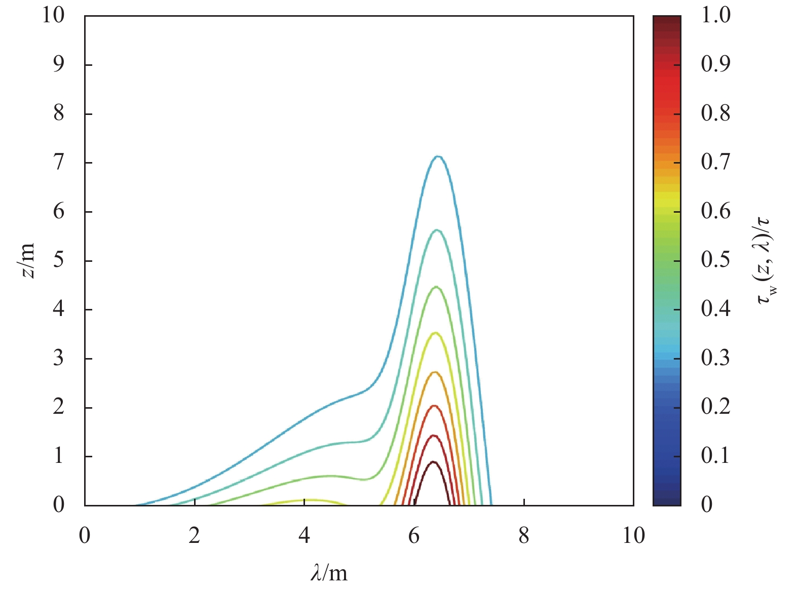
Figure 6 shows the dependence of wave stress on wave length and vertical coordinates. The results show that the wave length ranging from 5 to 7 m is effective in influencing the atmosphere. The wave boundary layer is always limited in 8 m.

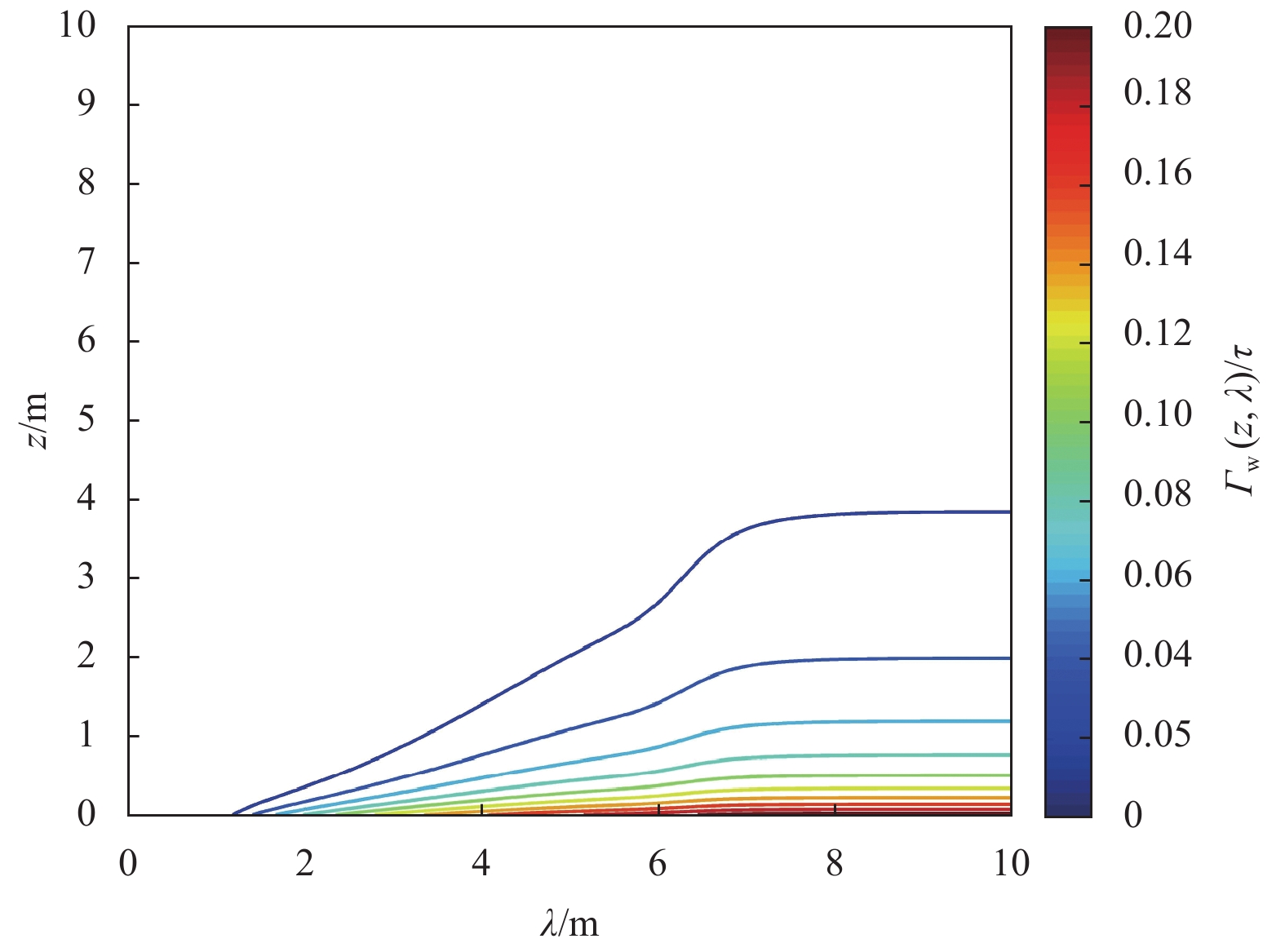
The contribution of waves to wave stress as a function of wave length and height is defined as
| $$ {\varGamma _{\rm{w}}}(z,\lambda) = \int_0^\lambda {{t_{\rm{w}}}} (z,\lambda){\rm{d}}\lambda, $$ | (16) |
and the results are shown in Fig. 7. For wave lengths smaller than approximately 7 m, Γw increases monotonically with λ, and when the wave length is greater than approximately 7 m, Γw appears to be constant, suggesting that wave length in this range contributes little to the total stress.

Figure 8 shows the drag coefficient changing with wind speed and wave age, andthe observational data are also shown. It can be seen that the influence of wave age on drag coefficient is significant and covers the range of observational drag coefficients. For low wind speed (U10N ≤ ~ 5 m/s), sea waves are too small to support large wave stress so that the total stress is almost provided by Eq. (9). Equation (9) shows that ocean roughness will increase with wind decrease because of friction velocity in the denominator. At this time, the sea surface is almost aerodynamically smooth; thus, the drag coefficient increases with a decrease in wind.

With the increase of wind speed (U10N≥~ 5 m/s), the wave dominates the ocean surface, and the drag coefficient begins to increase, but the slope of the drag coefficient depends on wave age. In the condition of larger cp/U10, which is larger than approximately 0.6, the result is similar to our observations in 6–11 m/s wind speed, which tend to be almost constant. When cp/U10 is below 0.6, the drag coefficient CDN is very sensitive to the U10N. CDN increases sharply with wind speed, which corresponds to our observation data for U10N>11 m/s.
As the viscous stress is negligible above the wave sublayer, it is very important to clarify the other two stresses in different conditions of wind speed. Smedman et al. (2003) proposed a wave boundary layer where the wave stress contributes to the total stress significantly. In pure wind conditions, the thickness of the wave boundary layer is only approximately 1 m (Janssen, 1989). However, it becomes much higher when the swell dominates in the field (Smedman et al., 1994; Grachev et al., 2003). Belcher and Hunt (1998) found that the wave-induced momentum flux from the ocean to the atmosphere is strongly related to the wave age cp/U10, where cp is the phase speed of the wave at the spectral peak. When cp/U10<1, the wind speed is greater than wave speed; therefore, the developing wind wave extracts momentum from the atmosphere. In this condition, the wind profiles above the surface follow logarithmic law. For cp/U10>1, the swells play a dominant role in the observational field. This may lead to the wave stress becoming negative and even the transfer of momentum from the ocean to the atmosphere. This hypothesis illuminates that a jet-like wind profile is obtained with a maximum at the height of the wave boundary layer.
The footprints of waves on wind stress are evidenced in the present study. These developing wind waves, which are characterized by steeper slopes and younger wave ages, provide a rougher surface that leads to greater CDN. The waves from the open sea are usually related to a long fetch and feature a smaller steepness, resulting in a smaller drag efficient.
We investigate the characteristics of air-sea momentum flux in the coastal ocean. The tower-based wind measurements are deployed at 20 m above the mean sea surface, and the sampling frequency is as high as 10 Hz. The time period starts from September 2010 and ends in August 2012. The eddy-correlation method is used to calculate the momentum flux. The tower is located 6.5 km distance to the coast, and the water depth is 14 m.
The influence of surface waves on air-sea momentum flux is evident in the present dataset. When we divided the wind conditions into an onshore case (corresponding to large wave fetch) and an offshore case (corresponding to small wave fetch), the momentum flux was significantly different. Our results underpin the wind-wave interaction theory that the air-sea momentum flux is correlated to the surface wave.
A parameterization scheme is examined for the wave-affected air-sea momentum flux. The scheme takes into account the wave effects in terms of wave spectrum. The differences between fetch-limited waves and saturated waves are consistent with the observations.
The results emphasize the dependence of air-sea momentum flux on wave age. Benefiting from the wave spectrum, other than the dominant wave parameters as shown in previous studies (Taylor and Yelland, 2001), the parameterization scheme is supposed to contain more information on the surface wave. The new scheme is capable of characterizing the air-sea momentum flux for low-to-moderate wind; however, because the wave spectrum used here is adopted from the JONSWAP spectrum, the scheme calls for further quantitative validation in the future.
| [1] |
Babanin A V, Makin V K. 2008. Effects of wind trend and gustiness on the sea drag: Lake George study. Journal of Geophysical Research: Oceans, 113(C2): C02015
|
| [2] |
Belcher S E, Hunt J C R. 1998. Turbulent flow over hills and waves. Annual Review of Fluid Mechanics, 30: 507–538. doi: 10.1146/annurev.fluid.30.1.507
|
| [3] |
Bumke K, Schlundt M, Kalisch J, et al. 2014. Measured and parameterized energy fluxes estimated for Atlantic transects of R/V Polarstern. Journal of Physical OceanographyJ Phys Oceanogr, 44(2): 482–491. doi: 10.1175/JPO-D-13-0152.1
|
| [4] |
Bye J A T, Jenkins A D. 2006. Drag coefficient reduction at very high wind speeds. Journal of Geophysical Research: Oceans, 111(C3): C03024
|
| [5] |
Charnock H. 1955. Wind stress on a water surface. Quarterly Journal of the Royal Meteorological Society, 81(350): 639–640
|
| [6] |
Chen Sheng, Qiao Fangli, Huang Chuanjiang, et al. 2018. Deviation of wind stress from wind direction under low wind conditions. Journal of Geophysical Research: Oceans, 123(12): 9357–9368. doi: 10.1029/2018JC014137
|
| [7] |
Desjardins R L, MacPherson J I, Schuepp P H, et al. 1989. An evaluation of aircraft flux measurements of CO2, water vapor and sensible heat. Boundary-Layer Meteorology, 47(1–4): 55–69
|
| [8] |
Donelan M A, Babanin A V, Young I R, et al. 2006. Wave-follower field measurements of the wind-input spectral function. Part II: parameterization of the wind input. Journal of Physical Oceanography, 36(8): 1672–1689. doi: 10.1175/JPO2933.1
|
| [9] |
Donelan M A, Haus B K, Reul N, et al. 2004. On the limiting aerodynamic roughness of the ocean in very strong winds. Geophysical Research Letters, 31(18): L18306. doi: 10.1029/2004GL019460
|
| [10] |
Drennan W M, Graber H C, Hauser D, et al. 2003. On the wave age dependence of wind stress over pure wind seas. Journal of Geophysical Research: Oceans, 108(C3): 8062. doi: 10.1029/2000JC000715
|
| [11] |
Edson J, Crawford T, Crescenti J, et al. 2007. The coupled boundary layers and air-sea transfer experiment in low winds. Bulletin of the American Meteorological Society, 88(3): 341–356. doi: 10.1175/BAMS-88-3-341
|
| [12] |
Edson J B, Jampana V, Weller R A, et al. 2013. On the exchange of momentum over the open ocean. Journal of Physical Oceanography, 43(8): 1589–1610. doi: 10.1175/JPO-D-12-0173.1
|
| [13] |
Fairall C W, Bradley E F, Hare J E, et al. 2003. Bulk parameterization of air–sea fluxes: updates and verification for the COARE algorithm. Journal of Climate, 16(4): 571–591. doi: 10.1175/1520-0442(2003)016<0571:BPOASF>2.0.CO;2
|
| [14] |
Frederickson P A, and Davidson K L. 2003. Observational buoy studies of coastal air-sea fluxes. Journal of Climate, 16(4): 593–599. doi: 10.1175/1520-0442(2003)016<0593:OBSOCA>2.0.CO;2
|
| [15] |
Garratt J R. 1977. Review of drag coefficients over oceans and continents. Monthly Weather Review, 105(7): 915–929. doi: 10.1175/1520-0493(1977)105<0915:RODCOO>2.0.CO;2
|
| [16] |
Geernaert G L. 1988. Measurements of the angle between the wind vector and wind stress vector in the surface layer over the North Sea. Journal of Geophysical Research: Oceans, 93(C7): 8215–8220. doi: 10.1029/JC093iC07p08215
|
| [17] |
Grachev A A, Fairall C W, Hare J E, et al. 2003. Wind stress vector over ocean waves. Journal of Physical Oceanography, 33(11): 2408–2429. doi: 10.1175/1520-0485(2003)033<2408:WSVOOW>2.0.CO;2
|
| [18] |
Grare L, Lenain L, Melville W K. 2013. Wave-coherent airflow and critical layers over ocean waves. Journal of Physical Oceanography, 43(10): 2156–2172. doi: 10.1175/JPO-D-13-056.1
|
| [19] |
Greenhut G K, Khalsa S J S. 1995. Bulk transfer coefficients and dissipation-derived fluxes in low wind speed conditions over the western equatorial Pacific Ocean. Journal of Geophysical Research: Oceans, 100(C1): 857–863. doi: 10.1029/94JC02256
|
| [20] |
Hanley K E, Belcher S E. 2008. Wave-driven wind jets in the marine atmospheric boundary layer. Journal of the Atmospheric Sciences, 65(8): 2646–2660. doi: 10.1175/2007JAS2562.1
|
| [21] |
Hanley K E, Belcher S E, Sullivan P P. 2010. A global climatology of wind–wave interaction. Journal of Physical Oceanography, 40(6): 1263–1282. doi: 10.1175/2010JPO4377.1
|
| [22] |
He Hailun, Song Jinbao, Bai Yefei, et al. 2018a. Climate and extrema of ocean waves in the East China Sea. Science China Earth Sciences, 61(7): 980–994. doi: 10.1007/s11430-017-9156-7
|
| [23] |
He Hailun, Wu Qiaoyan, Chen Dake, et al. 2018b. Effects of surface waves and sea spray on air-sea fluxes during the passage of typhoon Hagupit. Acta Oceanologica Sinica, 37(5): 1–7. doi: 10.1007/s13131-018-1208-2
|
| [24] |
He Hailun, Xu Yao. 2016. Wind-wave hindcast in the Yellow Sea and the Bohai Sea from the year 1988 to 2002. Acta Oceanologica Sinica, 35(3): 46–53. doi: 10.1007/s13131-015-0786-5
|
| [25] |
Huang Yansong, Song Jinbao, Fan Conghui. 2013. A motion correction on direct estimations of air-sea fluxes from a buoy. Acta Oceanologica Sinica, 32(3): 63–70. doi: 10.1007/s13131-013-0290-8
|
| [26] |
Janssen P A E M. 1989. Wave-induced stress and the drag of air flow over sea waves. Journal of Physical Oceanography, 19(6): 745–754. doi: 10.1175/1520-0485(1989)019<0745:WISATD>2.0.CO;2
|
| [27] |
Kudryavtsev V N. 2006. On the effect of sea drops on the atmospheric boundary layer. Journal of Geophysical Research: Oceans, 111(C7): C07020
|
| [28] |
Kudryavtsev V N, Makin V K. 2007. Aerodynamic roughness of the sea surface at high winds. Boundary-Layer Meteorology, 125(2): 289–303. doi: 10.1007/s10546-007-9184-7
|
| [29] |
Large W G, Pond S. 1981. Open ocean momentum flux measurements in moderate to strong winds. Journal of Physical Oceanography, 11(3): 324–336. doi: 10.1175/1520-0485(1981)011<0324:OOMFMI>2.0.CO;2
|
| [30] |
Mahrt L, Vickers D., Howell J, et al. 1996. Sea surface drag coefficients in the Risø Air Sea Experiment. Journal of Geophysical Research: Oceans, C(6): 14327–14335
|
| [31] |
Makin V K. 2005. A note on the drag of the sea surface at hurricane winds. Boundary-Layer Meteorology, 115(1): 169–176. doi: 10.1007/s10546-004-3647-x
|
| [32] |
Makin V K, Kudryavtsev V N. 1999. Coupled sea surface-atmosphere model: 1. Wind over waves coupling. Journal of Geophysical Research: Oceans, 104(C4): 7613–7623
|
| [33] |
Makin V K, Kudryavtsev V N, Mastenbroek C. 1995. Drag of the sea surface. Boundary-Layer Meteorology, 73(1–2): 159–182
|
| [34] |
Moncrieff J, Clement R, Finnigan J, et al. 2004. Averaging, detrending, and filtering of eddy covariance time series. In: Lee X, Massman W, Law B, eds. Handbook of Micrometeorology: A Guide for Surface Flux Measurement and Analysis. Dordrecht: Springer, 7–31
|
| [35] |
Monin A S, Yaglom A M. 1971. Statistical Fluid Mechanics. Cambridge, MA: MIT Press, 417–526
|
| [36] |
Oncley S P, Friehe C A, Larue J C, et al. 1996. Surface-layer fluxes, profiles, and turbulence measurements over uniform terrain under near-neutral conditions. Journal of the Atmospheric Sciences, 53(7): 1029–1044. doi: 10.1175/1520-0469(1996)053<1029:SLFPAT>2.0.CO;2
|
| [37] |
Paulson C A, Leavitt E, Fleagle R G. 1972. Air-sea transfer of momentum, heat and water determined from profile measurements during BOMEX. Journal of Physical Oceanography, 2(4): 487–497. doi: 10.1175/1520-0485(1972)002<0487:ASTOMH>2.0.CO;2
|
| [38] |
Pedlosky J. 1964. The stability of currents in the atmosphere and the ocean: part I. Journal of the Atmospheric Sciences, 21(2): 201–219. doi: 10.1175/1520-0469(1964)021<0201:TSOCIT>2.0.CO;2
|
| [39] |
Pedreros R, Dardier G, Dupuis H, et al. 2003. Momentum and heat fluxes via the eddy correlation method on the R/V L’Atalante and an ASIS buoy. Journal of Geophysical Research: Oceans, 108(C11): 3339. doi: 10.1029/2002JC001449
|
| [40] |
Peng S Q, Xie L, Pietrafesa L J. 2007. Correcting the errors in the initial conditions and wind stress in storm surge simulation using an adjoint optimal technique. Ocean Modelling, 18(3–4): 175–193
|
| [41] |
Powell M D, Vickery P J, Reinhold T A. 2003. Reduced drag coefficient for high wind speeds in tropical cyclones. Nature, 422(6929): 279–283. doi: 10.1038/nature01481
|
| [42] |
Price J F. 1981. Upper ocean response to a hurricane. Journal of Physical Oceanography, 11(2): 153–175. doi: 10.1175/1520-0485(1981)011<0153:UORTAH>2.0.CO;2
|
| [43] |
Semedo A, Saetra Ø, Rutgersson A, et al. 2009. Wave-induced wind in the marine boundary layer. Journal of the Atmospheric Sciences, 66(8): 2256–2271. doi: 10.1175/2009JAS3018.1
|
| [44] |
Sjöblom A, Smedman A S. 2004. Comparison between eddy-correlation and inertial dissipation methods in the marine atmospheric surface layer. Boundary-Layer Meteorology, 110(2): 141–164. doi: 10.1023/A:1026006402060
|
| [45] |
Smedman A S, Guo Larsén X, Högström U, et al. 2003. Effect of sea state on the momentum exchange over the sea during neutral conditions. Journal of Geophysical Research: Oceans, 108(C11): 3367. doi: 10.1029/2002JC001526
|
| [46] |
Smedman A S, Tjernström M, Högström U. 1994. The near-neutral marine atmospheric boundary layer with no surface shearing stress: a case study. Journal of the Atmospheric Sciences, 51(23): 3399–3411. doi: 10.1175/1520-0469(1994)051<3399:TNNMAB>2.0.CO;2
|
| [47] |
Smith S D. 1980. Wind stress and heat flux over the ocean in gale force wind. Journal of Physical Oceanography, 10(5): 709–726. doi: 10.1175/1520-0485(1980)010<0709:WSAHFO>2.0.CO;2
|
| [48] |
Smith S D, Anderson R J, Oost W A, et al. 1992. Sea surface wind stress and drag coefficients: the HEXOS results. Boundary-Layer Meteorology, 60(1–2): 109–142
|
| [49] |
Song Jinbao, Fan Wei, Li Shuang, et al. 2015. Impact of surface waves on the steady near-surface wind profiles over the ocean. Boundary-Layer Meteorology, 155(1): 111–127. doi: 10.1007/s10546-014-9983-6
|
| [50] |
Song Jinbao, Huang Yansong. 2011. An approximate solution of wave-modified Ekman current for gradually varying eddy viscosity. Deep Sea Research Part I: Oceanographic Research Papers, 58(6): 668–676. doi: 10.1016/j.dsr.2011.04.001
|
| [51] |
Sullivan P P, Edson J B, Hristov T, et al. 2008. Large-eddy simulations and observations of atmospheric marine boundary layers above nonequilibrium surface waves. Journal of the Atmospheric Sciences, 65(4): 1225–1245. doi: 10.1175/2007JAS2427.1
|
| [52] |
Sun Jielun, Nappo C J, Mahrt L, et al. 2015. Review of wave-turbulence interactions in the stable atmospheric boundary layer. Reviews of Geophysics, 53(3): 956–993. doi: 10.1002/2015RG000487
|
| [53] |
Tamura H, Drennan W M, Sahlée E, et al. 2014. Spectral form and source term balance of short gravity wind waves. Journal of Geophysical Research: Oceans, 119(11): 7406–7419. doi: 10.1002/2014JC009869
|
| [54] |
Taylor P K, Yelland M J. 2001. The dependence of sea surface roughness on the height and steepness of the waves. Journal of Physical Oceanography, 31(2): 572–590. doi: 10.1175/1520-0485(2001)031<0572:TDOSSR>2.0.CO;2
|
| [55] |
Vickers D, Mahrt L, Andreas E L. 2013. Estimates of the 10-m neutral sea surface drag coefficient from aircraft eddy-covariance measurements. Journal of Physical Oceanography, 43(2): 301–310. doi: 10.1175/JPO-D-12-0101.1
|
| [56] |
Wang Shihong, Liu Zhiliang, Pang Chongguang, et al. 2016. The decadally modulating eddy field in the upstream Kuroshio Extension and its related mechanisms. Acta Oceanologica Sinica, 35(5): 9–17. doi: 10.1007/s13131-015-0741-5
|
| [57] |
Wang Juanjuan J, Song Jinbao, Huang Yansong, et al. 2013. Application of the Hilbert-Huang Transform to the estimation of air-sea turbulent fluxes. Boundary-Layer Meteorology, 147(3): 553–568. doi: 10.1007/s10546-012-9784-8
|
| [58] |
Weill A, Eymard L, Caniaux G, et al. 2003. Toward a better determination of turbulent air-sea fluxes from several experiments. Journal of Climate, 16(4): 600–618. doi: 10.1175/1520-0442(2003)016<0600:TABDOT>2.0.CO;2
|
| [59] |
Wu Jin. 1980. Wind-stress coefficients over sea surface near neutral conditions—A revisit. Journal of Physical Oceanography, 10(5): 727–740. doi: 10.1175/1520-0485(1980)010<0727:WSCOSS>2.0.CO;2
|
| [60] |
Xu Yao, He Hailun, Song Jinbao, et al. 2017. Observations and modeling of typhoon waves in the South China Sea. Journal of Physical Oceanography, 47(6): 1307–1324. doi: 10.1175/JPO-D-16-0174.1
|
| [61] |
Yelland M, Taylor P K. 1996. Wind stress measurements from the open ocean. Journal of Physical Oceanography, 26(4): 541–558. doi: 10.1175/1520-0485(1996)026<0541:WSMFTO>2.0.CO;2
|
| [62] |
Young I R. 1999. Wind Generated Ocean Waves. Amsterdam: Elsevier, 45–62
|
| [63] |
Zhang Ting, Song Jinbao. 2018. Effects of sea-surface waves and ocean spray on air-sea momentum fluxes. Advances in Atmospheric Sciences, 35(4): 469–478. doi: 10.1007/s00376-017-7101-7
|
| [64] |
Zhang Ting, Song Jinbao, Li Shuang, et al. 2016. The effects of wind-driven waves and ocean spray on the drag coefficient and near-surface wind profiles over the ocean. Acta Oceanologica Sinica, 35(11): 79–85. doi: 10.1007/s13131-016-0950-6
|
| [65] |
Zou Zhongshui, Zhao Dongliang, Huang Jian, et al. 2014. The analysis and application of estimation methods for air-sea interface momentum flux. Haiyang Xuebao (in Chinese), 36(9): 75–83
|
| [66] |
Zou Zhongshui, Zhao Dongliang, Liu Bin, et al. 2017. Observation-based parameterization of air-sea fluxes in terms of wind speed and atmospheric stability under low-to-moderate wind conditions. Journal of Geophysical Research: Oceans, 122(5): 4123–4142. doi: 10.1002/2016JC012399
|
| [67] |
Zou Zhongshui, Zhao Dongliang, Zhang Juna, et al. 2018. The influence of swell on the atmospheric boundary layer under nonneutral conditions. Journal of Physical Oceanography, 48(4): 925–936. doi: 10.1175/JPO-D-17-0195.1
|


Figures(8)

Supported by:
Beijing Renhe Information Technology Co. Ltd


 DownLoad:


 DownLoad: