
Figure
1.
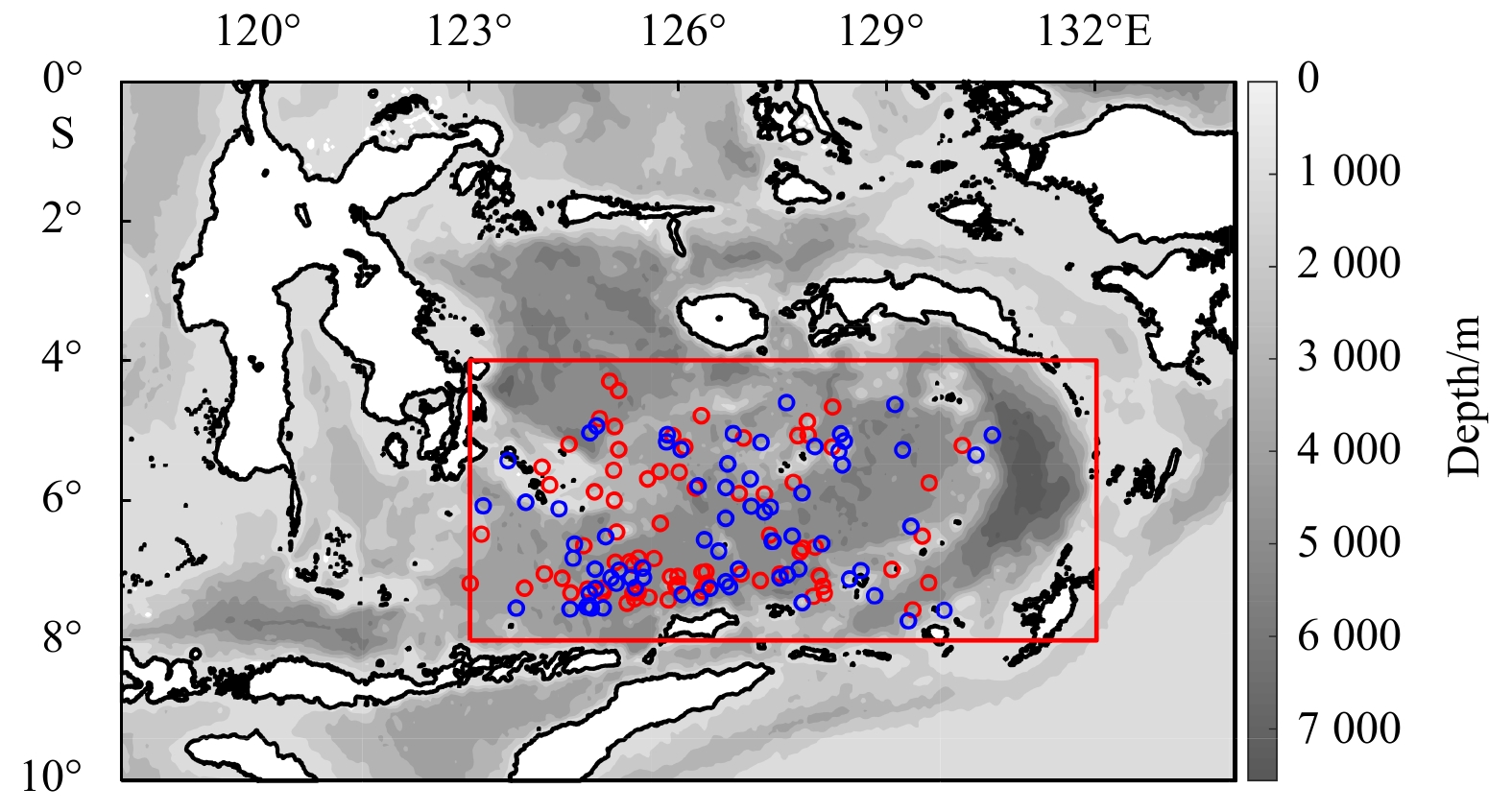
Map of the Banda Sea and adjacent Indonesian seas. Green, red and yellow arrow lines represent the west, central and east pathways of the ITF, respectively.
| Citation: | Baiyang Chen, Lingling Xie, Quanan Zheng, Lei Zhou, Lei Wang, Baoxin Feng, Zipeng Yu. Seasonal variability of mesoscale eddies in the Banda Sea inferred from altimeter data[J]. Acta Oceanologica Sinica, 2020, 39(12): 11-20. doi: 10.1007/s13131-020-1665-2

|
Mesoscale eddies with typical horizontal scales of O(100) km are broadly distributed in the global oceans (McDowell and Rossby, 1978; Zheng and Yuan, 1989; Chelton et al., 2011; Shi et al., 2018). They carry 90% of kinetic energy of the ocean and play an important role in mass and energy transports, biogeochemistry and climate change (Chen et al., 2012; Zhang et al., 2013; Xu et al., 2016; Frenger et al., 2018). Thus, mesoscale eddies have become a research hotspot in ocean dynamics, ocean ecology and marine environmental sciences (Benitez-Nelson et al., 2007; Zhang et al., 2014; McGillicuddy, 2016; Yang et al., 2019).
In recent years, mesoscale eddies in the northwest Pacific (NWP) and the South China Sea (SCS) have attracted much attention (Wang et al., 2005; Wu and Chiang, 2007; Qiu and Chen, 2010; Hu et al., 2012; Lin et al., 2012; Yang et al., 2013; Xie et al., 2016, 2018; Zheng et al., 2017, 2019). Previous investigators have analyzed statistical characteristics of mesoscale eddies using satellite data, in-situ observations and numerical simulations (Wang et al., 2003; Xiu et al., 2010; Chen et al., 2011; Hu et al., 2011; Li et al., 2011; Zhang et al., 2016; Qiu et al., 2019). Lin (2005) analyzed the seasonal variability of number, lifespan, radius and speed of mesoscale eddies in the NWP and the SCS using satellite altimeter sea level anomaly (SLA) data from 1993 to 2001. Zheng et al. (2014) analyzed statistical features of mesoscale eddies in the North Pacific. Zheng et al. (2017) reviewed progress in the research of mesoscale eddies in the SCS over past 60 a. In addition to the surface-intensified ones, subsurface (or subthermocline) eddies that have cores and transports in the subsurface layer have also been recognized (e.g., Zhang et al., 2015, 2019; Li et al., 2017; Nan et al., 2019; Xu et al., 2019).
The Indonesian seas are an important channel for water exchange between the Pacific and the Indian Ocean (Wang et al., 2016b; Wang et al., 2018). The Indonesian Throughflow (ITF) flowing through this channel is a key link in the thermohaline circulation (Broecker, 1991; Gordon, 2005) and plays an important role in the global climate change (Du and Fang, 2011; Sprintall et al., 2014). The Banda Sea located at 4°–8°S, 123°–132°E in the southeastern Indonesian seas is an important channel for the ITF as shown in Fig. 1. It is a deep basin with a total area of 470 000 km2, an average depth of 3 064 m and the deepest depth of 7 440 m. It connects to the Molukka Sea and is a key ocean area for the eastern pathway of the ITF, where the larger uncertainty of transport exists (Talley and Sprintall, 2005; Van Aken et al., 2009; Wang et al., 2019).
The circulation and mesoscale eddies in the Banda Sea are important for understanding the variability of the mass and heat transports of the ITF (Gordon and Susanto, 2001; Feng and Wijffels, 2002; Wang et al., 2019). Previous studies have investigated the basin circulation in the Banda Sea through numerical simulation and found that the climatological circulation is clockwise in the surface and bottom layers and counterclockwise in the middle layer (Liang et al., 2019). Gordon and Susanto (2001) investigated the seasonal variability of the sea surface temperature (SST) in the Banda Sea and found SST is lower in boreal summer than that in boreal winter. The sea level also has a great seasonal variability, higher in winter and spring and lower in summer and autumn, with an annual variation range reaching 16.5 cm (Wang et al., 2016a). However, the characteristics of mesoscale eddies and their seasonal variability remain unclear.
This study aims to exploring the statistical characteristics of surface-intensified mesoscale eddies (mesoscale eddies for short, hereafter) in the Banda Sea using 24 a global mesoscale eddy trajectory product derived from the satellite altimeter data. Meanwhile, the mechanisms for seasonal polarity distribution reversal (PDR) phenomenon of mesoscale eddies are examined with reanalysis data of ocean currents and winds. It is expected that the results of this study can help understanding the dynamic processes of the ITF and the biogeochemical processes in the Banda Sea.
The global mesoscale eddy trajectory atlas product derived from satellite altimeter absolute dynamic topography (ADT) and sea level anomaly (SLA) data are used as a baseline for this study. The dataset is provided by Archiving, Validation and Interpretation of Satellite Oceanography Data (AVISO) (
(1) The number of connected pixels n≤nmax (a specified maximum number);
(2) n≥2, a minimum of two interior pixels in an eddy;
(3) no pixel in an eddy can have a neighbor pixel that belongs to another eddy;
(4) the pixels in the eddy are simply connects, i.e., there is no “holes” in the eddy;
(5) the distance between the extremum pixel and pixels in the eddy has a maximum value dmax.
The five criteria were chosen to yield eddies that are statistically similar to those using the method of Chelton et al. (2011). For the AVISO SSH field, nmax is chosen to be 2 000. dmax is 400 km at mid latitudes and 700 km in equator. An additional constrain that eddies must have amplitude A≥1 cm was also imposed. Details on the detection algorithm can be found in Schlax and Chelton (2016).
Previous investigators have used similar satellite altimeter data products for studies of dynamic processes in the Banda Sea. For examples, Gordon and Susanto (2001) used the altimeter data derived from combined TOPEX Poseidon (T/P) and European Research Satellite (ERS) sea-level anomaly (SLA) products to analyze the Banda Sea surface-layer divergence. Wang et al. (2016a) analyzed the seasonal and interannual variations of the sea level height in the Banda Sea based on combined T/P, Janson-1/2 and ERS-1/2 satellite altimeter absolute dynamic topography (ADT) products. Thus, the validated global mesoscale eddy trajectory atlas product should be suitable or even better for analyzing mesoscale eddies in the Banda Sea.
The ocean current data sets used are the Simple Ocean Data Assimilation (SODA v3.3.1) reanalysis monthly average data (
This study also uses the ERA-Interim numerical forecast reanalyzed monthly average 10 m winds downloaded from the European Centre for Medium-Range Weather Forecasts (ECMWF) (
From global mesoscale eddy dataset, eddies in the Banda Sea from 1 January 1993 to 31 December 2016 are selected. For the statistical analysis, eddies are grouped into four boreal seasons, i.e., winter (December–February), spring (March–May), summer (June–August) and autumn (September–November). The average position of eddy is defined as the average latitude and longitude during its survival time. The propagation speed of eddy is calculated by the distance that eddy moves per day.
The seasonal mean ocean currents are calculated from the monthly average ocean current data of SODA from 1993 to 2015. The seasonal mean vorticity is calculated from the seasonal mean ocean current velocity as
The seasonal mean winds are calculated using the same methods. The seasonal wind stress curl is calculated by
Figure 2 shows the average positions of mesoscale eddies in the Banda Sea from 1993 to 2016. During the 24 years, there were 147 mesoscale eddies occurred, of which 137 eddies were locally generated and 10 originated from outside. The total number of cyclonic eddies (CEs, clockwise in the southern hemisphere), 76, is close to 71 of anticyclonic eddies (AEs, anticlockwise in the southern hemisphere). Figure 2 indicates that eddies are concentrated gradually from the northern to the southern Banda Sea. CEs and AEs have similar distribution patterns.

Table 1 lists statistics of kinematic parameters of eddies in the Banda Sea. One can see that the average survival time of AEs is 40 d and that of CEs is 41 d. The average radius is 116 km. The average SLA amplitude (magnitude of the height difference between the extremum of SLA within the eddy and the SLA around the contour defining the eddy perimeter) is 4.1 cm. The average rotation speed is 40.8 cm/s. CEs with the average amplitude of 4.5 cm and the average rotation speed of 43.5 cm/s are stronger than 3.7 cm and 38.0 cm/s of AEs. The average propagation speeds are 16.8 cm/s for the total, 16.0 cm/s for CEs and 17.5 cm/s for AEs. The total AEs and CEs generally have similar properties except that the amplitude and rotating speed of the CEs are 20% stronger and the propagation speed is 9% slower.
| Number | Survival time/d | Amplitude/cm | Radius/km | Propagation speed/cm·s–1 | Rotation speed/cm·s–1 | |
| CEs (clockwise) | 76 | 41 | 4.5 | 116 | 16.0 | 43.5 |
| AEs (anticlockwise) | 71 | 40 | 3.7 | 116 | 17.5 | 38.0 |
| Total | 147 | 40 | 4.1 | 116 | 16.8 | 40.8 |
 DownLoad:
CSV
DownLoad:
CSV
Tables 2 and 3 list the seasonal variability of eddy parameters in the Banda Sea, show that the total number of mesoscale eddies in the Banda Sea is 56 in winter and 60 in spring and decreases to 42 in summer and autumn. In winter, the number of CEs is 39, about 2.3 times 17 of AEs. In contrast, in summer, the number of AEs is 30, about 2.5 times 12 of CEs. Though the total numbers of AEs and CEs are similar (Table 1), the seasonal distribution of AEs and CEs are completely reversal.
| Number | Seasonal survival time/d | Amplitude/cm | Radius/km | Propagation speed/cm·s–1 | Rotation speed/cm·s–1 | |
| Winter | 56 | 31 | 4.6 | 115 | 15.4 | 44.2 |
| Spring | 60 | 30 | 4.3 | 120 | 16.3 | 41.4 |
| Summer | 42 | 28 | 3.6 | 112 | 17.5 | 38.8 |
| Autumn | 42 | 27 | 3.5 | 114 | 18.3 | 36.3 |
| Average | 50 | 29 | 4.0 | 115 | 16.9 | 40.2 |
| STD | ±10 | ±2 | ±0.5 | ±3 | ±1.3 | ±3.4 |
| ±20% | ±7% | ±12% | ±3% | 8% | 8% |
DownLoad:
CSV
| Number | Seasonal survival time/d | Amplitude/cm | Radius/km | Propagation speed/cm·s–1 | Rotation speed/cm·s–1 | |
| Winter | 17 (39) | 29 (32) | 3.2 (5.2) | 103 (120) | 15.6 (15.3) | 41.3 (45.7) |
| Spring | 33 (27) | 29 (32) | 3.9 (4.8) | 124 (115) | 19.0 (14.0) | 39.6 (43.3) |
| Summer | 30 (12) | 26 (32) | 3.9 (3.1) | 113 (112) | 16.7 (19.0) | 36.9 (42.8) |
| Autumn | 20 (22) | 28 (25) | 3.5 (3.5) | 117 (110) | 17.9 (18.9) | 33.5 (39.4) |
| Average | 25 (25) | 28 (30) | 3.6 (4.2) | 114 (114) | 17.3 (16.8) | 37.8 (42.8) |
| STD | ±8 (±11) | ±1 (±4) | ±0.3 (±1.0) | ±9 (±4) | ±1.5 (±2.5) | ±3.4 (±2.6) |
| 32% (44%) | 4% (13%) | 8% (24%) | 8% (4%) | 9% (15%) | 9% (6%) |
DownLoad:
CSV
The seasonal average survival time of mesoscale eddies reaches a maximum of 31 d in winter, and gradually reduces to 27 d in autumn. It is 32 d in winter, spring, and summer, and reduces to 25 d in autumn for CEs. The value of AEs is 29 d in winter and spring, 28 d in autumn, and 26 d in summer, respectively. The seasonal average survival time of CEs is 2 d longer than that of AEs. The seasonal average survival time is 10 d shorter than the total survival time, indicating that some eddies are generated in one season but dissipated in another season.
The total mean radius of mesoscale eddies in the Banda Sea is 115 km and the seasonal variation is small with standard deviation (STD) less than 3%. The radius of the AEs has a relatively lager STD of 8%. The average SLA amplitude of eddies is the largest 4.6 cm in winter, and gradually decreases to 3.5 cm in autumn. The average SLA amplitude of CEs reaches the maximum 5.2 cm in winter, while that of AEs reaches the minimum 3.2 cm. In summer, the average SLA amplitude of AEs reaches the highest 3.9 cm, while that CEs is the minimum 3.1 cm. The CEs are the strongest in winter and the weakest in summer, while the situation is reversal for the AEs.
The average propagation speed of eddies in the Banda Sea increases from 15.4 cm/s in winter to 18.3 cm/s in autumn, and the maximum propagation speed of AEs and CEs, 19.0 cm/s appear in spring and summer, respectively. The propagation speeds in summer for both the CEs and AEs are higher than that in winter. In contrast to the propagation speed, the average rotation speed of eddies in the Banda Sea is 40.2 cm/s with a decrease trend from winter to autumn. The average rotation speed of CEs is 42.8 cm/s, 13% greater than 37.8 cm/s of AEs.
In summary, the number of mesoscale eddies in the Banda Sea has remarkable seasonal variability with a STD of 20%, especially that the number of CEs has STD of 44%. The average survival time of about one month varies little in all seasons. The total average SLA amplitude is 4.0 cm with STD of 12%, and the STD of the average SLA amplitude of CEs reaches 24%. The average radius is 115 km with little change in all seasons. The average propagation speed of AEs is 17.3 cm/s, 3% faster than 16.8 cm/s of CEs, while the average rotation speed of CEs is 42.8 cm/s, 13% faster than 37.8 cm/s of the AEs. Most characteristics of the CEs have larger seasonal variation than that of the AEs.
Figure 3 shows the spatial distribution of mesoscale eddies and the sketch of ocean currents in different seasons in the Banda Sea. One can see that in winter 90% of CEs are distributed in the southern basin south of 6°S, and 76% of AEs in the central and northern basin. In summer, the reversed patterns happen, i.e., 83% of AEs are distributed in the southern basin and 90% of CEs in the northern basin. Spring and summer show transition distribution patterns. This is the PDR phenomenon of AEs and CEs in the Banda Sea. The sketches of ocean currents show the opposite directions, i.e., eastward in winter and westward in summer. The currents in spring and autumn are both westward and weaker than that in winter and summer. The seasonally reversed ocean currents may be a reason responsible for the PDR.

In order to show the seasonal PDR phenomenon of mesoscale eddies in the Banda Sea more clearly, we further show the spatial distribution patterns of the daily positions of mesoscale eddies in four seasons in Fig. 4. One can see that concentration of CEs and AEs alternate north-southward with changes in seasons, i.e., CEs in the south and AEs in the north in winter and spring, while CEs are in the north and the AEs are in the south in summer and autumn. This shows that the eddy polarities at the same location are reversed.

Figure 5 shows climatologically seasonal distribution of the upper ocean (5 m) currents and the relative vorticity of the horizontal current in the Banda Sea derived from the SODA data. One can see that in winter the ocean currents, especially in the south of 6°S, are dominated by the eastward flows, and the relative vorticity of the horizontal current shows north-south distribution patterns, i.e., negative in the south and positive in the north. The vorticity distribution patterns are generally consistent with the CE (negative vorticity) and AE (positive vorticity) distribution patterns as shown in Fig. 4. In spring, the currents in the south are still eastward, while that in the north of 5°S change to westward flows. In summer, the currents completely reverse from that in winter and the relative vorticity of the horizontal current distribution patterns in the south and the north also show an opposite situation, i.e., positive in the south and negative in the north. The vorticity distribution patterns are also closely related to the distribution patterns of CEs and AEs as shown in Fig. 4. In autumn, the currents are generally westward and the velocity in the central basin is weakened. In summary, the circulation patterns and flow directions in the Banda Sea reverse with the season, as well as the relative vorticity distribution patterns.

Figure 6 further shows the seasonal variability of the wind vectors and the wind stress curl in the Banda Sea derived from the ECMWF wind data. One can see that the wind vectors are mainly westerly in winter, and the wind stress curl shows north-south distribution patterns, i.e., negative in the south and positive in the north. The distribution patterns of the wind stress curl are consistent with that of CEs in the south and AEs in the north in winter as shown in Fig. 4. In summer, the easterly wind vectors prevail, and the wind stress curl distribution patterns in the south and north also show an opposite situation, i.e., positive in the south and negative in the north. One can see that the wind stress curl distribution patterns show a close relation to that of mesoscale eddies in summer as shown in Fig. 4. The intensity of wind stress curl in winter and summer is greater than that in spring and autumn, meanwhile that in summer is greater than that in winter. The westerly wind vectors are the strongest in winter. The wind stress curl in the southern basin becomes positive in spring and gradually develops to the patterns in summer. In autumn, the wind stress curl in the whole basin begins to decrease, and transforms into the patterns in winter, forming an annual cycle. One can see that the wind vectors and the variability of the wind stress curl are similar to the ocean current vectors and the relative vorticity of the horizontal current. Probably, it is the seasonal-reversal wind stress curl drives the seasonal-reversal basin-scale circulation, and then generates the PDR of mesoscale eddies in the Banda Sea.

As shown in Fig. 5, the Banda Sea currents have three distinctive features: (1) zonal flows are dominant in all seasons; (2) the direction of the zonal flow reverses with the season; (3) the relative vorticity (dominated by the meridional shear of zonal flow as described later) in the northern and southern basin reverse with the seasons.
Shi et al. (2018) proposed a solitary (eddy) solution based on an asymptotic expansion of the nonlinear potential vorticity equation with a constant meridional shear of zonal current. The used nondimensional potential vorticity equation is:
| $$ \frac{\partial }{\partial t}\left({\nabla }^{2}\psi -F\psi \right)+J\left(\psi,{\nabla }^{2}\psi \right)+\beta \frac{\partial \psi }{\partial x}=0, $$ | (1) |
where F= L2/R2 d, L is a characteristic length scale of the motion, Rd is the Rossby deformation radius,
| $$ \omega \approx \frac{3m\left|\beta +F{u}_{0}\right|}{\left({n}^{2}{\rm{{ π}}}^{2}+F\right)\sqrt{\varepsilon }}\frac{1}{\sqrt{\left[1-{\left(-1\right)}^{n}\right]n{\rm{{ π}}}}\sqrt{{A}_{0}\text{δ}}}, $$ | (2) |
where m represents the modulus of Jacobi elliptic function, n is the mode number of Rossby wave, u0 is the mean of zonal flow, δ represents the flow shear strength, and A0 is the amplitude of the solitary waves (i.e., eddies). This implies the width of the solitary wave is inversely proportional to the flow shear strength |δ|, and that (A0δ) must be positive to keep this width physical meaningful. In other words, if the background flow shear is positive (δ>0), A0 must be positive too. Positive A0 means there are anticyclonic (cyclonic) solitary Rossby waves (A0>0, n=1) in the Northern (Southern) Hemisphere. On the other hand, if it is negative (δ<0), there are cyclonic (anticyclonic) solitary Rossby waves (A0<0, n=1) in the Northern (Southern) Hemisphere.
According to the above analysis, cyclonic (anticyclonic) eddies can be generated by the positive (negative) shear of the zonal current in the Banda Sea. For zonal current v=0, the meridional shear just equals the minus of the vorticity
Furthermore, the distribution patterns of the ocean current vorticity (Fig. 5) and wind stress curl (Fig. 6) are consistent with that of CEs in the south and AEs in the north in winter as shown in Fig. 4, while there is an opposite situation in summer. One can see that the reversed wind stress curl and the corresponding reversal of basin-scale ocean current vorticity and meridional shear are possible mechanisms affecting the PDR.
Previous studies have shown that barotropic instability, baroclinic instability, and wind forcing are the main mechanisms for generating mesoscale eddies in the ocean (Gill et al., 1974; Frankignoul and Müller, 1979; Richardson, 1983; Pedlosky, 1987; Qiu et al., 2009; Zhang, 2014).
To clarify the dominant energy source for eddies in the Banda Sea, we investigate the composite baroclinic (BC) and barotropic (BT) eddy energy conversion rates and rate of wind stress work (WW). Here, BC, BT, and WW are defined, following that by Zhang et al. (2017)
| $$ {\rm{B}}{\rm{C}}=-\int\!\!\frac{{g}^{2}}{{\rho }_{0}{N}^{2}}v'\rho' \cdot {\nabla }_{\rm{{h}}}\stackrel{-}{\rho }{\rm{d}}z, $$ | (3) |
| $$ {\rm{B}}{\rm{T}}=-\int \!\!{\rho }_{0}\frac{\partial \stackrel{-}{{u}_{i}}}{\partial {x}_{i}}{u}_{i}'{u}_{j}'{\rm{d}}z, $$ | (4) |
and
| $$ {\rm{W}}{\rm{W}}={\tau }_{\rm{w}}{v'}_{0}, $$ | (5) |
where overbars and prime' denote time mean (12 months) and monthly anomalies from the climatologically time mean, g is the gravitational acceleration, N is the buoyancy frequency,
Figure 7 shows the time series of the spatial averaged BC, BT and WW in the south (6°–8°S) and north (4°–6°S) of the basin. One can see that in the southern basin, positive BCs are larger than BTs in winter and summer months, while BTs are greater than BCs in spring and autumn. In the northern basin, however, BCs are negative in most months except for summer. BTs dominate the eddy energy in the northern basin in winter, and also have at least half contribution in summer. The variability of WW in the southern and the northern basins are essentially the same, i.e., in most months are positive and the values in winter and summer are greater than that in spring and autumn, except the values in the southern basin are greater than that in the northern basin. The results in Fig. 7 suggest that in winter and summer, the energy sources for eddies are from wind forcing, barotropic instability and baroclinic instability of the mean flow in the southern basin, and mainly from wind forcing. In the northern basin, the energy sources in winter are from wind forcing and barotropic instability of the mean flow, while in summer from wind forcing, barotropic instability and baroclinic instability of the mean flow and primarily from wind forcing.

Previous studies have shown that the eddies in the South China Sea (SCS) are affected by ENSO (Chu et al., 2014, 2017). Both the Banda Sea and the SCS are important sea areas through which ITF flows, and ENSO is closely related to ITF. Thus, eddies in the Banda Sea may be affected by ENSO. To test this scenario, we compare ocean currents and daily eddy positions in the Banda Sea during the El Niño event from May 1997 to May 1998, and the La Niña from July 1998 to July 1999. The results are shown in Fig. 8. One can see that during the El Niño event the ocean currents flowed anticlockwise in the western basin and most eddies were distributed on the south and the east sides of the circulation, while during the La Niña event, the ocean currents flowed anticlockwise in the western basin, but clockwise in the eastern basin and eddies were distributed along the circulation. This indicates that the eddy distribution patterns are remarkable different during the El Niño and the La Niña events. This phenomenon is worth pursuing for the future efforts.

Using the global mesoscale eddy trajectory product derived from satellite altimeter data from 1993 to 2016, this study analyzes statistical characteristics and the seasonal PDR phenomenon of mesoscale eddies in the Banda Sea. The major conclusions are summarized as follows:
(1) During the 24 years, there were 147 mesoscale eddies (76 CEs and 71 AEs) observed. Among them 137 mesoscale eddies (93%) were generated inside the sea, and 10 of them (7%) originated outside the sea. The statistical means of eddies are as follows: the survival time of 40 d, the radius of 116 km, the SLA amplitude of 4.1 cm, the propagation speed of 16.8 cm/s, and the rotation speed of 40.8 cm/s. The survival time, amplitude and rotation speed of CEs are slightly greater than that of AEs, and the other properties are generally the same.
(2) There is the seasonal variability of mesoscale eddy properties. The number of eddies changes 20%, the average survival time, amplitude, and rotation speed gradually decrease from 7% to 12% from winter to autumn, and the propagation speed increases by 7%. There are significant differences between CE and AE characteristics in winter and summer. In winter, the number of CEs is 2.3 times that of AEs and the SLA amplitude is 1.6 times higher, while in summer, the number of AEs is 2.5 times that of CEs and the amplitude is 1.3 times. In winter and summer, the polarities of mesoscale eddies at the same location reverse. Similar phenomenon occurs in spring and autumn, but not as remarkable as in winter and summer.
(3) The analysis of background ocean currents and the winds reveals that the ocean currents of the Banda Sea may be driven by the wind stress curl. The ocean currents are dominated by the zonal currents. The directions of upper ocean currents and the vorticity polarities reverse in winter and summer. The wind vectors reverse in winter and summer, and the wind stress curl in the northern and the southern basins also reverse.
(4) The dynamic analysis indicates that wind forcing is the main mechanism for the eddy generation in the Banda Sea, while barotropic instability and baroclinic instability are also exist. The seasonal reversal of the meridional shear, basin-scale vorticity, and wind stress curl are possible mechanisms affecting the PDR.
The mesoscale eddy trajectory atlas product is downloaded from Archiving Validation and Interpretation of Satellite Data in Oceanography (AVISO), the Centre National d’Ettudes Spatiales (CNES) of France (
| [1] |
Benitez-Nelson C R, Bidigare R R, Dickey T D, et al. 2007. Mesoscale eddies drive increased silica export in the Subtropical Pacific Ocean. Science, 316(5827): 1017–1021. doi: 10.1126/science.1136221
|
| [2] |
Broecker W S. 1991. The great ocean conveyor. Oceanography, 4(2): 79–89. doi: 10.5670/oceanog.1991.07
|
| [3] |
Chelton D B, Schlax M G, Samelson R M. 2011. Global observations of nonlinear mesoscale eddies. Progress in Oceanography, 91(2): 167–216. doi: 10.1016/j.pocean.2011.01.002
|
| [4] |
Chen Gengxin, Gan Jianping, Xie Qiang, et al. 2012. Eddy heat and salt transports in the South China Sea and their seasonal modulations. Journal of Geophysical Research: Oceans, 117(C5): C05021
|
| [5] |
Chen Gengxin, Hou Yijun, Chu Xiaoqing. 2011. Mesoscale eddies in the South China Sea: Mean properties, spatiotemporal variability, and impact on thermohaline structure. Journal of Geophysical Research: Oceans, 116(C6): C06018
|
| [6] |
Chu Xiaoqing, Dong Changming, Qi Yiquan. 2017. The influence of ENSO on an oceanic eddy pair in the South China Sea. Journal of Geophysical Research: Oceans, 122(3): 1643–1652. doi: 10.1002/2016JC012642
|
| [7] |
Chu Xiaoqing, Xue Huijie, Qi Yiquan, et al. 2014. An exceptional anticyclonic eddy in the South China Sea in 2010. Journal of Geophysical Research: Oceans, 119(2): 881–897. doi: 10.1002/2013JC009314
|
| [8] |
Du Yan, Fang Guohong. 2011. Progress on the study of the Indonesian seas and Indonesian Throughflow (in Chinese). Advances in Earth Sciences, 26(11): 1131–1142
|
| [9] |
Feng Meng, Wijffels S. 2002. Intraseasonal variability in the South Equatorial Current of the East Indian Ocean. Journal of Physical Oceanography, 32(1): 265–277. doi: 10.1175/1520-0485(2002)032<0265:IVITSE>2.0.CO;2
|
| [10] |
Frankignoul C, Müller P. 1979. Quasi-geostrophic response of an infinite β-plane ocean to stochastic forcing by the atmosphere. Journal of Physical Oceanography, 9(1): 104–127. doi: 10.1175/1520-0485(1979)009<0104:QGROAI>2.0.CO;2
|
| [11] |
Frenger L, Münnich M, Gruber N. 2018. Imprint of Southern Ocean mesoscale eddies on chlorophyll. Biogeosciences, 15(15): 4781–4798. doi: 10.5194/bg-15-4781-2018
|
| [12] |
Gill A E, Green J S A, Simmons A J. 1974. Energy partition in the large-scale ocean circulation and the production of mid-ocean eddies. Deep Sea Research and Oceanographic Abstracts, 21(7): 499–528. doi: 10.1016/0011-7471(74)90010-2
|
| [13] |
Gordon A L. 2005. Oceanography of the Indonesian seas and their throughflow. Oceanography, 18(4): 14–27. doi: 10.5670/oceanog.2005.01
|
| [14] |
Gordon A L, Susanto R D. 2001. Banda Sea surface-layer divergence. Ocean Dynamics, 52(1): 2–10. doi: 10.1007/s10236-001-8172-6
|
| [15] |
Hu Jianyu, Gan Jianping, Sun Zhenyu, et al. 2011. Observed three-dimensional structure of a cold eddy in the southwestern South China Sea. Journal of Geophysical Research: Oceans, 116(C5): C05016
|
| [16] |
Hu Jianyu, Zheng Quanan, Sun Zhenyu, et al. 2012. Penetration of nonlinear Rossby eddies into South China Sea evidenced by cruise data. Journal of Geophysical Research: Oceans, 117(C3): C03010
|
| [17] |
Li Jiaxun, Zhang Ren, Jin Baogang, et al. 2011. Eddy characteristics in the northern South China Sea as inferred from Lagrangian drifter data. Ocean Science, 7(5): 661–669. doi: 10.5194/os-7-661-2011
|
| [18] |
Li Cheng, Zhang Zhiwei, Zhao Wei, et al. 2017. A statistical study on the subthermocline submesoscale eddies in the northwestern Pacific Ocean based on Argo data. Journal of Geophysical Research: Oceans, 122(5): 3586–3598. doi: 10.1002/2016JC012561
|
| [19] |
Liang Linlin, Xue Huijie, Shu Yeqiang. 2019. The Indonesian Throughflow and the circulation in the Banda Sea: A modeling study. Journal of Geophysical Research: Oceans, 124(5): 3089–3106. doi: 10.1029/2018JC014926
|
| [20] |
Lin Pengfei. 2005. Statistical analyses on mesoscale eddies in the South China Sea and the northwest Pacific (in Chinese)[dissertation]. Qingdao: Institute of Oceanology, Chinese Academy of Sciences
|
| [21] |
Lin Hongyang, Hu Jianyu, Zheng Quanan. 2012. Satellite altimeter data analysis of the South China Sea and the northwest Pacific Ocean: Statistical features of oceanic mesoscale eddies. Journal of Oceanography in Taiwan Strait (in Chinese), 31(1): 105–113
|
| [22] |
McDowell S E, Rossby H T. 1978. Mediterranean water: An intense mesoscale eddy off the Bahamas. Science, 202(4372): 1085–1087. doi: 10.1126/science.202.4372.1085
|
| [23] |
McGillicuddy D J Jr. 2016. Mechanisms of physical-biological-biogeochemical interaction at the oceanic mesoscale. Annual Review of Marine Science, 8: 125–159. doi: 10.1146/annurev-marine-010814-015606
|
| [24] |
Nan Feng, Yu Fei, Ren Qiang, et al. 2019. Isopycnal mixing of interhemispheric intermediate waters by subthermocline eddies east of the philippines. Scientific Reports, 9: 2957. doi: 10.1038/s41598-019-39596-2
|
| [25] |
Pedlosky J. 1987. Geophysical Fluid Dynamics. 2nd ed. New York: Springer-Verlag, 490–623
|
| [26] |
Qiu Bo, Chen Shuiming. 2010. Interannual variability of the North Pacific subtropical countercurrent and its associated mesoscale eddy field. Journal of Physical Oceanography, 40(1): 213–225. doi: 10.1175/2009JPO4285.1
|
| [27] |
Qiu Bo, Chen Shuiming, Kessler W S. 2009. Source of the 70-day mesoscale eddy variability in the Coral Sea and the North Fiji Basin. Journal of Physical Oceanography, 39(2): 404–420. doi: 10.1175/2008JPO3988.1
|
| [28] |
Qiu Chunhua, Mao Huabin, Liu Hailong, et al. 2019. Deformation of a warm eddy in the northern South China Sea. Journal of Geophysical Research: Oceans, 124(8): 5551–5564. doi: 10.1029/2019JC015288
|
| [29] |
Richardson P L. 1983. Eddy kinetic energy in the North Atlantic from surface drifters. Journal of Geophysical Research: Oceans, 88(C7): 4355–4367. doi: 10.1029/JC088iC07p04355
|
| [30] |
Schlax M G, Chelton D B. 2016. The “growing method” of eddy identification and tracking in two and three dimensions. Oregon: College of Earth, Ocean and Atmospheric Sciences, Oregon State University, Corvallis, Oregon, 1: 8
|
| [31] |
Shi Yunlong, Yang Dezhou, Feng Xingru, et al. 2018. One possible mechanism for eddy distribution in zonal current with meridional shear. Scientific Reports, 8: 10106. doi: 10.1038/s41598-018-28465-z
|
| [32] |
Sprintall J, Gordon A L, Koch-Larrouy A, et al. 2014. The Indonesian seas and their role in the coupled ocean-climate system. Nature Geoscience, 7(7): 487–492. doi: 10.1038/ngeo2188
|
| [33] |
Talley L D, Sprintall J. 2005. Deep expression of the Indonesian Throughflow: Indonesian intermediate water in the South Equatorial Current. Journal of Geophysical Research: Oceans, 110(C10): C10009. doi: 10.1029/2004JC002826
|
| [34] |
Van Aken H M, Brodjonegoro I S, Jaya I. 2009. The deep-water motion through the Lifamatola Passage and its contribution to the Indonesian throughflow. Deep Sea Research Part I: Oceanographic Research Papers, 56(8): 1203–1216. doi: 10.1016/j.dsr.2009.02.001
|
| [35] |
Wang Guihua, Su Jilan, Chu P C. 2003. Mesoscale eddies in the South China Sea observed with altimeter data. Geophysical Research Letters, 30(21): 2121. doi: 10.1029/2003GL018532
|
| [36] |
Wang Guihua, Su Jilan, Qi Yiquan. 2005. Advances in studying mesoscale eddies in South China Sea. Advances in Earth Sciences (in Chinese), 20(8): 882–886
|
| [37] |
Wang Liwei, Wang Yonggang, Xu Tengfei, et al. 2016a. Seasonal and interannual variation in sea level height in the Banda Sea based on satellite altimeter data. Oceanologia et Limnologia Sinica (in Chinese), 47(4): 719–729
|
| [38] |
Wang Xin, Wang Dongxiao, Zhang Chidong, et al. 2016b. Introduction to maritime continent observation plan and progress in China. Acta Meteorologica Sinica (in Chinese), 74(4): 653–654
|
| [39] |
Wang Lu, Xie Lingling, Zhou Lei, et al. 2018. Climatological analysis of water mass sources of Indonesia Throughflow in the Molukka Sea and Halmahera Sea. Haiyang Xuebao (in Chinese), 40(3): 1–15
|
| [40] |
Wang Lu, Zhou Lei, Xie Lingling, et al. 2019. Seasonal and interannual variability of water mass sources of Indonesian Throughflow in the Maluku Sea and the Halmahera Sea. Acta Oceanologica Sinica, 38(4): 58–71. doi: 10.1007/s13131-019-1413-7
|
| [41] |
Wu C R, Chiang T L. 2007. Mesoscale eddies in the northern South China Sea. Deep Sea Research Part II: Topical Studies in Oceanography, 54(14–15): 1557–1588
|
| [42] |
Xie Lingling, Zheng Quanan, Tian Jiwei, et al. 2016. Cruise observation of Rossby waves with finite wavelengths propagating from the Pacific to the South China Sea. Journal of Physical Oceanography, 46(10): 2897–2913. doi: 10.1175/JPO-D-16-0071.1
|
| [43] |
Xie Lingling, Zheng Quanan, Zhang Shuwen, et al. 2018. The Rossby normal modes in the South China Sea deep basin evidenced by satellite altimetry. International Journal of Remote Sensing, 39(2): 399–417. doi: 10.1080/01431161.2017.1384591
|
| [44] |
Xiu Peng, Chai Fei, Shi Lei, et al. 2010. A census of eddy activities in the South China Sea during 1993–2007. Journal of Geophysical Research: Oceans, 115(C3): C03012
|
| [45] |
Xu Lixiao, Li Peiliang, Xie Shangping, et al. 2016. Observing mesoscale eddy effects on mode-water subduction and transport in the North Pacific. Nature Communications, 7: 10505. doi: 10.1038/ncomms10505
|
| [46] |
Xu Anqi, Yu Fei, Nan Feng. 2019. Study of subsurface eddy properties in northwestern Pacific Ocean based on an eddy-resolving OGCM. Ocean Dynamics, 69(4): 463–474. doi: 10.1007/s10236-019-01255-5
|
| [47] |
Yang Qingxuan, Nikurashin M, Sasaki H, et al. 2019. Dissipation of mesoscale eddies and its contribution to mixing in the northern South China Sea. Scientific Reports, 9: 556. doi: 10.1038/s41598-018-36610-x
|
| [48] |
Yang Guang, Wang Fan, Li Yuanlong, et al. 2013. Mesoscale eddies in the northwestern subtropical Pacific Ocean: Statistical characteristics and three-dimensional structures. Journal of Geophysical Research: Oceans, 118(4): 1906–1925. doi: 10.1002/jgrc.20164
|
| [49] |
Zhang Zhengguang. 2014. Mesoscale eddy (in Chinese)[dissertation]. Qingdao: Ocean University of China
|
| [50] |
Zhang Zhengguang, Wang Wei, Qiu Bo. 2014. Oceanic mass transport by mesoscale eddies. Science, 345(6194): 322–324. doi: 10.1126/science.1252418
|
| [51] |
Zhang Zhiwei, Li Peiliang, Xu Lixiao, et al. 2015. Subthermocline eddies observed by rapid-sampling Argo floats in the subtropical northwestern Pacific Ocean in Spring 2014. Geophysical Research Letters, 42(15): 6438–6445. doi: 10.1002/2015GL064601
|
| [52] |
Zhang Zhiwei, Liu Zhiyu, Richards K, et al. 2019. Elevated diapycnal mixing by a subthermocline eddy in the western equatorial Pacific. Geophysical Research Letters, 46(5): 2628–2636. doi: 10.1029/2018GL081512
|
| [53] |
Zhang Zhiwei, Tian Jiwei, Qiu Bo, et al. 2016. Observed 3D structure, generation, and dissipation of oceanic mesoscale eddies in the South China Sea. Scientific Reports, 6: 24349. doi: 10.1038/srep24349
|
| [54] |
Zhang Zhiwei, Zhao Wei, Qiu Bo, et al. 2017. Anticyclonic eddy sheddings from Kuroshio Loop and the accompanying cyclonic eddy in the northeastern South China Sea. Journal of Physical Oceanography, 47(6): 1243–1259. doi: 10.1175/JPO-D-16-0185.1
|
| [55] |
Zhang Zhiwei, Zhao Wei, Tian Jiwei, et al. 2013. A mesoscale eddy pair southwest of Taiwan and its influence on deep circulation. Journal of Geophysical Research: Oceans, 118(12): 6479–6494. doi: 10.1002/2013JC008994
|
| [56] |
Zheng Quanan, Ho C R, Xie Lingling, et al. 2019. A case study of a Kuroshio main path cut-off event and impacts on the South China Sea in fall-winter 2013–2014. Acta Oceanologica Sinica, 38(4): 12–19. doi: 10.1007/s13131-019-1411-9
|
| [57] |
Zheng Quanan, Xie Lingling, Zheng Zhiwen, et al. 2017. Progress in research of mesoscale eddies in the South China Sea. Advances in Marine Science (in Chinese), 35(2): 131–158
|
| [58] |
Zheng Congcong, Yang Yuxing, Wang Faming. 2014. Spatial-temporal features of eddies in the North Pacific. Marine Sciences (in Chinese), 38(10): 105–112
|
| [59] |
Zheng Quanan, Yuan Yeli. 1989. Study on the analytical model of decay of mesoscale eddy on the continental shelf. Science China, 32(9): 1135–1143
|
| 1. | Faisal Amri, Ahmed Eladawy, Joko Prihantono, et al. Disentangling mechanisms behind emerged sea surface temperature anomalies in Indonesian seas during El Niño years: insights from closed heat budget analysis. Journal of Oceanography, 2024. doi:10.1007/s10872-024-00728-6 | |
| 2. | Zhanjiu Hao, Zhenhua Xu, Ming Feng, et al. Seasonal variability of eddy kinetic energy in the Banda Sea revealed by an ocean model: An energy budget perspective. Deep Sea Research Part II: Topical Studies in Oceanography, 2023, 211: 105320. doi:10.1016/j.dsr2.2023.105320 | |
| 3. | F Hamzah. Nitrate and phosphate profiles in the Banda Sea during the northwest monsoon. IOP Conference Series: Earth and Environmental Science, 2023, 1163(1): 012002. doi:10.1088/1755-1315/1163/1/012002 | |
| 4. | Juana López Martínez, Edgardo Basilio Farach Espinoza, Hugo Herrera Cervantes, et al. Long-Term Variability in Sea Surface Temperature and Chlorophyll a Concentration in the Gulf of California. Remote Sensing, 2023, 15(16): 4088. doi:10.3390/rs15164088 | |
| 5. | Fangjie Yu, Meiyu Wang, Sijia Qian, et al. Multisatellite observations of smaller mesoscale eddy generation in the Kuroshio Extension. Acta Oceanologica Sinica, 2022, 41(9): 137. doi:10.1007/s13131-022-1996-2 |


Figures(8) / Tables(3)

Supported by:
Beijing Renhe Information Technology Co. Ltd

Baiyang Chen, Lingling Xie, Quanan Zheng, Lei Zhou, Lei Wang, Baoxin Feng, Zipeng Yu. Seasonal variability of mesoscale eddies in the Banda Sea inferred from altimeter data[J]. Acta Oceanologica Sinica, 2020, 39(12): 11-20. doi: 10.1007/s13131-020-1665-2

| Number | Survival time/d | Amplitude/cm | Radius/km | Propagation speed/cm·s–1 | Rotation speed/cm·s–1 | |
| CEs (clockwise) | 76 | 41 | 4.5 | 116 | 16.0 | 43.5 |
| AEs (anticlockwise) | 71 | 40 | 3.7 | 116 | 17.5 | 38.0 |
| Total | 147 | 40 | 4.1 | 116 | 16.8 | 40.8 |
DownLoad:
CSV
| Number | Seasonal survival time/d | Amplitude/cm | Radius/km | Propagation speed/cm·s–1 | Rotation speed/cm·s–1 | |
| Winter | 56 | 31 | 4.6 | 115 | 15.4 | 44.2 |
| Spring | 60 | 30 | 4.3 | 120 | 16.3 | 41.4 |
| Summer | 42 | 28 | 3.6 | 112 | 17.5 | 38.8 |
| Autumn | 42 | 27 | 3.5 | 114 | 18.3 | 36.3 |
| Average | 50 | 29 | 4.0 | 115 | 16.9 | 40.2 |
| STD | ±10 | ±2 | ±0.5 | ±3 | ±1.3 | ±3.4 |
| ±20% | ±7% | ±12% | ±3% | 8% | 8% |
DownLoad:
CSV
| Number | Seasonal survival time/d | Amplitude/cm | Radius/km | Propagation speed/cm·s–1 | Rotation speed/cm·s–1 | |
| Winter | 17 (39) | 29 (32) | 3.2 (5.2) | 103 (120) | 15.6 (15.3) | 41.3 (45.7) |
| Spring | 33 (27) | 29 (32) | 3.9 (4.8) | 124 (115) | 19.0 (14.0) | 39.6 (43.3) |
| Summer | 30 (12) | 26 (32) | 3.9 (3.1) | 113 (112) | 16.7 (19.0) | 36.9 (42.8) |
| Autumn | 20 (22) | 28 (25) | 3.5 (3.5) | 117 (110) | 17.9 (18.9) | 33.5 (39.4) |
| Average | 25 (25) | 28 (30) | 3.6 (4.2) | 114 (114) | 17.3 (16.8) | 37.8 (42.8) |
| STD | ±8 (±11) | ±1 (±4) | ±0.3 (±1.0) | ±9 (±4) | ±1.5 (±2.5) | ±3.4 (±2.6) |
| 32% (44%) | 4% (13%) | 8% (24%) | 8% (4%) | 9% (15%) | 9% (6%) |
DownLoad:
CSV
| Number | Survival time/d | Amplitude/cm | Radius/km | Propagation speed/cm·s–1 | Rotation speed/cm·s–1 | |
| CEs (clockwise) | 76 | 41 | 4.5 | 116 | 16.0 | 43.5 |
| AEs (anticlockwise) | 71 | 40 | 3.7 | 116 | 17.5 | 38.0 |
| Total | 147 | 40 | 4.1 | 116 | 16.8 | 40.8 |
| Number | Seasonal survival time/d | Amplitude/cm | Radius/km | Propagation speed/cm·s–1 | Rotation speed/cm·s–1 | |
| Winter | 56 | 31 | 4.6 | 115 | 15.4 | 44.2 |
| Spring | 60 | 30 | 4.3 | 120 | 16.3 | 41.4 |
| Summer | 42 | 28 | 3.6 | 112 | 17.5 | 38.8 |
| Autumn | 42 | 27 | 3.5 | 114 | 18.3 | 36.3 |
| Average | 50 | 29 | 4.0 | 115 | 16.9 | 40.2 |
| STD | ±10 | ±2 | ±0.5 | ±3 | ±1.3 | ±3.4 |
| ±20% | ±7% | ±12% | ±3% | 8% | 8% |
| Number | Seasonal survival time/d | Amplitude/cm | Radius/km | Propagation speed/cm·s–1 | Rotation speed/cm·s–1 | |
| Winter | 17 (39) | 29 (32) | 3.2 (5.2) | 103 (120) | 15.6 (15.3) | 41.3 (45.7) |
| Spring | 33 (27) | 29 (32) | 3.9 (4.8) | 124 (115) | 19.0 (14.0) | 39.6 (43.3) |
| Summer | 30 (12) | 26 (32) | 3.9 (3.1) | 113 (112) | 16.7 (19.0) | 36.9 (42.8) |
| Autumn | 20 (22) | 28 (25) | 3.5 (3.5) | 117 (110) | 17.9 (18.9) | 33.5 (39.4) |
| Average | 25 (25) | 28 (30) | 3.6 (4.2) | 114 (114) | 17.3 (16.8) | 37.8 (42.8) |
| STD | ±8 (±11) | ±1 (±4) | ±0.3 (±1.0) | ±9 (±4) | ±1.5 (±2.5) | ±3.4 (±2.6) |
| 32% (44%) | 4% (13%) | 8% (24%) | 8% (4%) | 9% (15%) | 9% (6%) |
 DownLoad:


 DownLoad: