Nitrogen fixation driven by mesoscale eddies and the Kuroshio Current in the northern South China Sea and the East China Sea

1. Introduction

Nitrogen is an essential macronutrient for marine phytoplankton growth, yet most of the world ocean is deficient in dissolved inorganic nitrogen (DIN) (Canfield et al., 2010). In the oligotrophic ecosystems, biological nitrogen fixation, a process participates by a selected group of microorganisms termed as diazotrophs, becomes the major source of new nitrogen to sustain marine primary production (Church and Böttjer, 2013; Benavides and Voss, 2015). Unlike other nitrogen sources, such as upwelling and diffusional flux of DIN, biological nitrogen fixation provides a pathway that input “new” nitrogen to upper waters dispense with CO₂ backflow from the deep ocean, and it is propitious to achieve net sequestration of atmospheric CO₂ (Eppley and Peterson, 1979). From a global perspective, the dynamics of marine nitrogen inventory depend on the difference between gains and losses of bioavailable nitrogen.

The South China Sea (SCS) and the East China Sea (ECS) are primary marginal seas in the western Pacific. As one of the largest marginal sea, the SCS occupies an important position that connects the Pacific Ocean and the India Ocean through the Bashi Channel, Sulu Sea, Malacca Strait (Wong et al., 2007). The SCS displays a complicated eco-hydrological conditions due to the interaction of monsoonal winds and eddies (Liu et al., 2002). Oligotrophic water, high sea surface temperature and persistent stratification make the SCS an ideal habitat to support the growth of diazotrophs (Kong et al., 2011). Indeed, it has been estimated that N₂ fixation rates (NFR) from diazotrophs contributed about 10% of total primary production (PP, in terms of C) and up to 20% of nitrogen inventory in the SCS (Voss et al., 2006; Gaye et al., 2009). The ECS is another China marginal sea affected by the Kuroshio intrusion, which transports large amounts of heat from south to north (Liu et al., 2002). The abundances of phytoplankton and zooplankton communities in the SCS and ECS are distinct with the difference in water temperatures (Shiozaki et al., 2015b). Trichodesmium spp. blooms were frequently observed in the Kuroshio Current (KC) in the summer while rarely occurred in the SCS basin (Lee Chen et al., 2008; Shiozaki et al., 2015b). In addition to temperature, the nitracline depth is another factor that impacts the abundance of diazotrophs in the Kuroshio (Shiozaki et al., 2014). Nitracline is usually shallower in the SCS than that in the Kuroshio, thereby nitrate is not easily accessible for non-diazotrophs, but for diazotrophs, especially Trichodesmium spp., they have a natural advantage in the Kuroshio (Shiozaki et al., 2014). Nevertheless, the high abundance of Trichodesmium spp. in the Kuroshio is still a subject of research and additional research approaches are needed to resolve this question.

Given the distinct and related biogeographic conditions within the SCS and ECS, we hypothesize that mesoscale processes and the Kuroshio intrusion were of vital importance to biogeochemical pathways in these adjacent areas. However, compared with the North Atlantic Ocean (Falcón et al., 2002; Luo et al., 2012; Agawin et al., 2013, 2014; Benavides and Voss, 2015) and the North Pacific Ocean (Montoya et al., 2004; Needoba et al., 2007; White et al., 2013), studies of the relationship between N₂ fixation and the driven force of mesoscale eddies as well as the Kuroshio intrusion were not sufficient (Voss et al., 2006; Lee Chen et al., 2008, 2014; Liu et al., 2013; Shiozaki et al., 2015a, 2018; Cheung et al., 2017). In the present study, we investigated the NFR in the summer and winter, as well as the PP in the same sampling stations. Our aims are (1) to study the spatiotemporal distributions of NFR in the northern South China Sea (nSCS) and the ECS under distinct mesoscale conditions; and (2) to estimate the contributions of NFR to PP varied with physical forces in two different seasons.

2. Materials and methods

2.1 Station locations, sampling and physicochemical analysis

The present study was conducted during two cruises in the nSCS and the ECS (15°–35°N, 105°–130°E), including a summer cruise from July 19 to August 16, 2009 and a winter cruise from December 23, 2009 to February 5, 2010. Occupied in 11 and 15 stations during the summer and winter cruise, samples for NFR measurement were classified into four categories according to their bottom depths and locations (Fig. 1): the nSCS shelf (Stations S209, D503, D104, E502a, A4 and S501a), the nSCS basin (Stations E607, A10, SEATS and LE09), the Luzon Strait (Stations S412, E401, E404 and E406), and ECS (Stations DH54, DH27b, PN04, DH11, PN05, DH37 and DH53).

Figure  1.  Sampling stations of N₂ fixation rates (NFR) in the northern South China Sea (nSCS) and the East China Sea (ECS) during the summer (a) and winter (b) cruises. Arrows indicate the Kuroshio intrusion path along the ECS and the nSCS. Solid line and dash line represent the degree of Kuroshio intrusion into the SCS in the two seasons (solid, winter; dash, summer). KMC, Kuroshio Main Current; KBC, Kuroshio Branch Current.

DownLoad: Full-Size Img PowerPoint

The vertical profiles of temperature and salinity were recorded by a Seabird CTD (Conductivity, Temperature and Depth; Sea-Bird Electronics, Washington, USA). The water samples for biochemical analysis were collected from 3–5 depths using a rosette water sampler (12 L Go-Flo bottles). Water samples for nutrient analysis were pre-filtered using 0.45 μm pore-size acetate fiber membranes. The filtrates were subsampled in 100 mL HCl-rinsed polyethylene (PE) bottles, and refrigerated at –20°C until further analysis. Nutrient analysis including nitrate (${\rm {NO}}_3^- $), nitrite (${\rm {NO}}_2^- $), phosphate (${\rm {PO}}_4^{3-} $) and silicate (${\rm {SiO}}_3^{2-} $) were estimated using Technicon AA3 Auto-Analyzer (Bran+ Luebbe, Germany) onboard according to colorimetric methods (Armstrong et al., 1967; Bernhardt and Wilhelms, 1967). The detection limits of ${\rm {NO}}_2^- $, ${\rm {NO}}_3^- $+${\rm {NO}}_2^- $, ${\rm {PO}}_4^{3-} $ and ${\rm {PO}}_4^{3-} $ concentrations were 0.04 µmol/L, 0.1 µmol/L, 0.08 µmol/L and 0.6 µmol/L, respectively.

Samples for chlorophyll a (Chl a) concentrations analysis were collected in 1 L PE bottles and gently filtered onto 25 mm GF/F filters (Waterman, USA). The filters were packed in aluminum foil and kept at –20°C during the cruise and detected immediately when came back to the laboratory. Pigments were extracted in the dark by adding 90% acetone for 24 h in a freezer. Further, Chl a concentrations were measured using Turner-Designs Trilogy^TM laboratory fluorometer (Turner Designs, USA).

2.2 Nitrogen fixation rates measurement

Estimation of NFR was carried out using acetylene reduction assay (ARA) described in Capone (1993). All cultivating experiments were run in triplicate, and GF/F filtered seawater was also incubated in triplicate as blank groups in each depth. Finally, NFR were corrected by its respective blank values. In each station, acetylene used in the experiments was generated from calcium carbide by adding Milli-Q water in a reaction flask. The generated gas was transferred into 1 L air tight belt through polypropylene valves.

In the summer cruise, 500 mL of seawater sample was introduced into a 600 mL HCl-rinsed polycarbonate bottle and sealed with a butyl rubber stopper. After sealing, 20 mL of acetylene was injected into the bottle by replacing the same volume of headspace. All bottles were subsequently incubated for 24 h in an on-deck incubator with running circulating waters pumped up from 5 m depth to maintain ambient temperature. After incubation, 0.2 mL saturated HgCl₂ was injected into each vial to end the N₂ fixation activities. Due to the logistical constraints, only in the South East Asia time-series study (SEATS) site, N₂ fixation incubations were conducted in different layers. While in the winter cruise, we conducted the cultivating experiments at all the sampling stations including different layers. The muti-layers sampling was based on different photosynthetically active radiation (PAR) at various depths, which accounted for 100%, 50%, 10%, 3% and 1% of the surface PAR, respectively. While several stations (Station A10 and stations in the ECS) only experimented at 100%, 10% and 1% layers due to logistical restriction. Incubation bottles were covered with distinct neutral density filters to simulate corresponding in-situ light intensity. Meanwhile, a modified method was used in the winter cruise experiment. About 180–750 mL samples were collected from different depths and filtrate concentrated to 12.5–50 times by Whatman^TM GF/F filters. The filters were placed in 25 mL glass vials and humidified with 15 mL GF/F filtered seawater. The vials were sealed with rubber stopper and aluminum caps by a crimper. Then, 2 mL of acetylene was injected into the bottle by a syringe. All the incubation experiments were performed on deck as described above.

The content of gas phase in the container was determined in the laboratory by a gas chromatograph (GC6890N, Agilent, USA) equipped with a flame ionization detector (FID). The column was wide–bore fused silica (20 m length, 0.53 mm inner diameter, 0.70 mm outside diameter) packed with Porapak U (Agilent, USA). The carrier gas was helium, and the flow rate was maintained at 9 mL/min, whereas the supply of hydrogen and air for the FID were maintained at 30 mL/min and 300 mL/min, respectively. The temperatures of the injector, detector and oven were set at 250°C, 200°C and 60°C, respectively. The quantity of sampling was 100 μL extracted from containers by a gastight syringe (Agilent, USA). The produced ethylene was converted to NFR by a theoretical converting factor of 4:1 that derived from equations as mentioned in Stal (1988):

2.3 Sea surface mesoscale features

Based on satellite datasets, the distribution pattern of mesoscale eddies and the Kuroshio were characterized to explain the distinct spatial-temporal allocation of nitrogen fixation activities in the SCS and ECS. Geostrophic sea water velocity was used to depict the distribution pattern of mesoscale-eddies or the Kuroshio Current in the summer nSCS, the winter nSCS, the summer ECS and the winter ECS. The geostrophic currents for the specific periods of mesoscale features were retrieved from the Copernicus Marine Environment Monitoring Service database (CMEMS) (http://marine.copernicus.eu/). Indicating the geographical positions of sampling station and the values of surface NFR, proportional white solid circle were overlaid on the merged images of the geostrophic currents. Given the uncertain variation of mesoscale features in daily scales, we select proper days which were mostly closed to survey schedule to represent the actual overall characters.

2.4 Primary production

The surface PP in the summer was measured by ¹⁴C method and calculated according to Parsons et al. (1984). Surface seawater samples were filled into 250 mL HCl-rinsed polycarbonate bottles (Nalgene, USA), and then 10 μCi NaH¹⁴CO₃ was added into each bottle. Each sample was incubated for 4 h in an on-deck incubator with running circulating water to maintain ambient temperature. At the end of the incubations, samples were filtered through pre-combusted 25 mm GF/F filters. The filters were packed in aluminum foil and kept at –20°C until further analysis. In the laboratory, the filters were transferred into the scintillation vials and acidified with 0.2 mL of 1 mol/L HCl to remove inorganic carbon. After 24 h in the fume hood, 5 mL scintillation cocktail (Ultima Gold, PerkinElmer, USA) were added, and the scintillation counter (Tri-Carb 2800TR, PerkinElmer, USA) were used to determine the total amount of added NaH¹⁴CO₃ (100%).

The vertically generalized production model (VGPM) was introduced in our study to calculate the depth-integrated primary production (IPP) in both seasons. Behrenfeld and Falkowski (1997) discovered a consistent trend in the vertical distribution of primary productivity through analyzing thousands of in suit ¹⁴C-based measured dates. The simplified equation of VGPM shows as follows:

where ${P^{\rm{B}}_{{\rm{opt}}}}$ and $Z_{{\rm{eu}}}$ are defined as a function of surface temperature and Chl a concentration, respectively.

Detailed information of symbols are shown in the Table 1.

Table  1.  Description of symbols in vertically generalized production model (VGPM)

Symbol	Data range	Description
$PP_{{\rm{eu}}}$/mg·m–2·d–1	−	depth-integrated primary productivity in terms of C
${P^{\rm{B}}_{{\rm{opt}}}}$/mg·mg–1·h–1	2.798−6.627	maximum optimum biomass-specific photosynthesis rate
$E_{\rm{o}}$/mol·m–2·d–1	3.396−57.412	surface daily photosynthetically available radiation (PAR) in terms of photons
$Z_{{\rm{eu}}}$/m	11.399−119.85	euphotic zone depth
$C_{{\rm{opt}}}$/mg·m–3	0.026−43.412	the sea surface chlorophyll a concentration
$D_{{\rm{irr}}}$/h	9.98−13.22	length of the day time
T/°C	9.2−30	the seawater temperature at each depth
Note: ${P^{\rm{B}}_{{\rm{opt}}}} $, the carbon content was produced by per milligram chlorophyll a per hour during photosynthesis.

 | Show Table

DownLoad: CSV

2.5 Statistical analysis

A normality test was performed before the significance test. We found that most of our data did not fit a normal distribution. So the significance tests in this study were calculated using nonparametric Mann-Whitney U test according to SPSS Statistics for Windows v.25.0 (IBM, USA). We performed significance tests between the value of NFR and the existences of physical process (anticyclonic eddies (AE), cyclonic eddies or no-eddy (CEONE) or KC) near our sampling station to reveal the relationship between NFR and physical process. The significance tests were also calculated to depict the seasonal pattern of physicochemical conditions.

3. Results

3.1 Physicochemical conditions

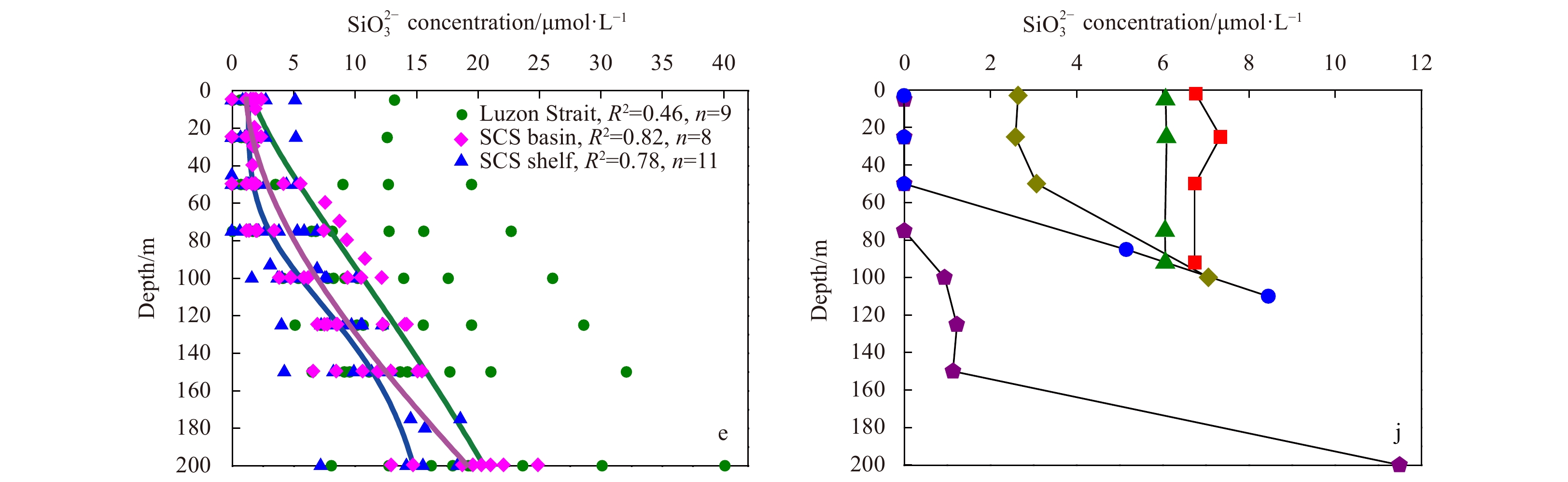
The horizontal distributions of temperature, salinity,${\rm {NO}}_3^- $+${\rm {NO}}_2^- $ concentration, ${\rm {PO}}_4^{3-} $ concentration, and ${\rm {SiO}}_3^{2-} $ concentration in the two seasons are shown in Table 2 and the vertical distributions are shown in Fig. 2. Surface temperature ranged from 28.63°C to 29.89°C (SCS: mean= (29.30±0.39)°C; ECS: mean= (29.13±0.54)°C) in the summer and 18.54°C to 25.83°C (SCS: mean= (24.37±0.94)°C; ECS: mean= (20.62±2.12)°C) in the winter. Surface salinity varied between 33.57 and 34.61, and was higher in winter, but lower in summer (32.79–34.05). The surface ${\rm {NO}}_3^- $+${\rm {NO}}_2^- $ and Chl a concentrations in the summer nSCS were significantly lower than that in the winter nSCS (P<0.05). While ${\rm {PO}}_4^{3-} $ concentration presented a converse trend in the two season (P<0.05). The average ${\rm {SiO}}_3^{2-} $concentration in the summer nSCS and winter nSCS were 2.22 µmol/L and 1.28 µmol/L, respectively.

Table  2.  Sea surface temperature (T), salinity (S), ${\rm {NO}}_3^- $+${\rm {NO}}_2^- $ (N+N, detection limit: 0.1 µmol/L), ${\rm {SiO}}_3^{2-} $ (detection limit: 0.16 µmol/L, ${\rm {PO}}_4^{3-} $(detection limit: 0.08 µmol/L), and chlorophyll a (Chl a, detection limit: 0.02 µg/L) in the northern South China Sea (nSCS) and the East China Sea (ECS) during the summer cruise and the winter cruise

Station	Date (day/ month/year)	T/°C	S	N+N concentration/ µmol·L–1	${\rm{SiO}}_3^{2-}$ concentration/ µmol·L–1	${\rm {PO}}_4^{3-} $ concentration/ µmol·L–1	Chl a concentration/ μg·L–1
S209	30/07/2009	29.50	33.56	0.1	0.72	0	0.08
D503	24/07/2009	29.69	33.55	0	8.70	0	0.09
D104	21/07/2009	29.63	33.49	0	0.41	0	0.03
E406	13/08/2009	29.24	32.79	0.1	2.56	0.09	0.37
LE09	13/08/2009	28.81	33.42	0	1.17	0.09	0.36
E607	26/07/2009	29.53	33.45	0	1.61	0	0.04
E404	14/08/2009	29.33	33.32	0	0.98	0.09	0.51
SEATS	11/08/2009	28.63	33.25	0.1	1.62	0.08	0.38
PN04	26/08/2009	29.89	33.62	0	1.95	0	0.70
DH54	19/08/2009	28.74	34.05	0.1	0.83	0.09	0.26
DH27b	21/08/2009	28.77	33.62	0.1	0.73	0	0.30
PN05	27/12/2009	18.83	34.02	4.2	6.06	0.33	0.34
DH37	30/12/2009	22.49	34.61	0.4	0	0	0.35
DH27b	30/12/2009	23.20	34.58	0.6	0	0	0.28
DH53	03/01/2010	20.04	34.53	2.3	2.64	0.16	0.81
E607	11/01/2010	24.50	33.87	0.2	1.39	0	0.44
SEATS	12/01/2010	24.66	33.72	0	2.41	0	0.19
A10	16/01/2010	24.09	33.80	0.2	1.71	0	0.53
A4	19/01/2010	22.78	34.49	0.6	1.10	0	0.43
S501a	21/01/2010	23.24	34.13	0.3	0.88	0	0.67
S412	27/01/2010	24.27	33.80	0	1.75	0	0.51
E406	27/01/2010	25.83	33.57	0.3	1.58	0	0.26
E404	28/01/2010	25.26	33.57	0.2	0.72	0	0.61
E401	30/01/2010	24.72	34.47	0.1	0	0	0.43
DH11	25/12/2009	18.54	34.11	4.1	6.78	0.12	0.30
E502a	11/01/2010	NA	NA	NA	NA	NA	NA
Note: 0 means the value is lower than the detection limit. NA indicates environmental parameters data at Station E502a were missed.

 | Show Table

DownLoad: CSV

Figure  2.  Vertical distribution of temperature, salinity, ${\rm {NO}}_3^- $+${\rm {NO}}_2^- $ concentration (detection limit: 0.100 µmol/L), ${\rm {PO}}_4^{3-} $concentration (detection limit: 0.080 µmol/L) and ${\rm {SiO}}_3^{2-}$ concentration (detection limit: 0.160 µmol/L) in the northern South China Sea (nSCS) (a, b, c, d, e, respectively) and the East China Sea (ECS) (f, g, h, i, j, respectively) during the winter cruise.

DownLoad: Full-Size Img PowerPoint

3.2 Horizontal distribution of nitrogen fixation rates

NFR in surface seawater ranged from 1.14 nmol/(L·d) to 10.40 nmol/(L·d) with an average of (4.89±3.46) nmol/(L·d) in the summer. However, in the winter, NFR in surface seawater performed a wider range, varying between 0.74 nmol/(L·d) to 29.45 nmol/(L·d) with an average of (7.81±8.50) nmol/(L·d). The maximum NFR in the summer and in the winter were recorded at Station D104 (anticyclonic eddy) and DH11 (eutrophic waters affected by runoffs, RW), respectively.

Given the dramatic variation of NFR in different area, a specific functional regional division based on different physical control were constructed to analyze the seasonal variation of NFR. As shown in Fig. 3a, in the summer nSCS, three stations (D104, S209, SEATS) were located at the edge of the AE, and one station (E404) was affected by the Kuroshion branch, while other three stations were not characterized with obvious physical features. On the contrary, in the winter nSCS (Fig. 3b), five stations were distributed around cyclonic eddies or with no obvious mesoscale features (CEONE), and stations (E401, E404, S412) located at the Luzon Strait were principally affected by Kuroshio intrusion. Notably, Station E406 was mainly controlled by Philippine offshore current in both seasons, and Station A10 located at a transition area reflected the combination of Kuroshio intrusion and oligotrophic SCS water. Compared with nSCS, the physical features in another marginal sea ECS were extraordinarily distinct. With rarely occurred mesoscale eddies, Kuroshio intrusion, as well as runoff effect, were the major physical forces in the study area. In detail, DH54 which was affected by Kuroshio Branch Current (KBC), DH27b which was affected by Kuroshio Main Current area (KMC), and PN04, a station representing the RW, were three stations corresponding to typical physical features in the summer ECS. Similarly, stations in the winter ECS were divided into KMC (DH27b, DH37) and RW (DH11, PN05, DH53).

Figure  3.  The surface N₂ fixation rates (NFR) and geostrophic sea water velocity (m/s) are merged to depict the impact of physical features on N₂ fixation in the northern South China Sea (nSCS) and the East China Sea (ECS): the summer nSCS (a, 1 August 2009), the winter nSCS (b, 23 January 2010), the summer ECS (c, 1 August 2009), and the winter ECS (d, 25 December 2009). The anticyclonic eddies are marked with red circles, while cyclonic eddies are marked with orange circles. The sizes of white dots are proportional to the values of NFR.

DownLoad: Full-Size Img PowerPoint

Significant correlations between the distribution patterns of mesoscale eddies and NFR were observed that the AE performed significantly higher NFR than that in the CEONE (P<0.01) (Figs 3a, b). Meanwhile, significantly higher NFR were also observed in the KBC or the KMC than that in the CEONE (P<0.05). However, no obvious discrepancy were observed between the AE and the KC. In the summer ECS, high NFR were recorded at DH54 which was affected by KBC, while NFR in the KMC (DH27b) were quite low compared to DH54 (Fig. 3c). The ECS recorded higher surface NFR than the SCS in the winter (P<0.05) (Fig. 3d). Both the KMC (DH27b and DH37) and RW (DH11, DH53) performed considerably high NFR.

3.3 Vertical distribution of nitrogen fixation rates

In the winter, the depth-integrated N₂ fixation rates (INF, in terms of N) ranged from 52.4 μmol/(m²·d) to 905.2 μmol/(m²·d), and the mean value was (428.9±305.5) μmol/(m²·d). Depth profiles of NFR in the winter are shown in Fig. 4. The vertical profiles of NFR were more fluctuate in the ECS and the Luzon Strait, implying dramatic variations of NFR in different layers. Meanwhile, the maximum value of NFR were observed frequently in the shallow water above 30 m. At Station DH11, the vertical profile of NFR were distinctly higher than ambient stations. While the trend changed along the nSCS basin and shelf, where high NFR were observed in deeper layer (30–80 m) at several stations (Stations E502a, A4 and A10), corresponding the gradually weakenKuroshio intrusion.

Figure  4.  Vertical distribution of the N₂ fixation rates (NFR) in the winter (a–d) and summer (b, SEATS). nSCS, northern South China Sea; ECS, East China Sea.

DownLoad: Full-Size Img PowerPoint

At Station SEATS in the nSCS basin, NFR in different layers were measured in the two distinct seasons to reflect the seasonal variation of dinitrogen fixation. As shown in Fig. 4b, the rates ranged from 0.76 nmol/(L·d) to 5.55 nmol/(L·d) in the summer. The 65 m depths recorded the highest NFR. While in the winter, the rates at Station SEATS ranged from 0.74 nmol/(L·d) to 7.12 nmol/(L·d), and the maximum NFR was observed at 50 m depth. Notably, two maximum NFR were observed at similar depth (50 m and 65 m). Calculated INF at Station SEATS experienced little difference in the two seasons, with 277.3 μmol/(m²·d) in the summer and 269.0 μmol/(m²·d) in the winter, respectively.

3.4 Primary production

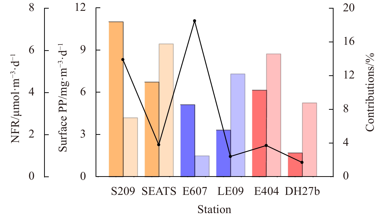
In the summer, the PP of six stations were measured in the surface water by ¹⁴C method. The surface PP ranged between 1.47 mg/(m³·d) and 9.44 mg/(m³·d) with an average of (6.06±3.01) mg/(m³·d). The maximum and minimum surface PP values were observed at Station SEATS and Station E607, respectively. Regretfully, due to the limitation of experiment, the ¹⁴C method was not used in the winter cruise to measure the surface PP. Based on VGPM model, IPP was calculated in the two seasons (Fig. 5). From a temporal perspective, the IPP was higher in the winter than that in the summer.

Figure  5.  Depth-integrated primary production (IPP) in the summer (a) and winter (b). Note that the sizes and colors of different circles corresponding to the values of IPP at different stations.

DownLoad: Full-Size Img PowerPoint

4. Discussion

4.1 The relationship between mesoscale eddies and nitrogen fixation rates

Given the significant consistence of NFR and mesoscale eddies as well as the Kuroshio intrusion path (P<0.01) (Figs 3a, b), we hypothesized that NFR in our study were mainly controlled by physical-biological force. Our NFR allocation results were equivalent to the distribution pattern of mesoscale eddies in the SCS that AE frequently occurred in summer while cyclonic eddies occurred continually in winter (Xue et al., 2004; Wang et al., 2008). We presumed that AE were probably responsible for the high NFR in the summer. Accompanying with anticyclonic eddy, warm oligotrophic surface water was transported downward where Trichodesmium spp. were not inhibited by light intensity (Jyothibabu et al., 2017). In addition, the downward vertical water mass movement may further weaken the upward transport of nutrients from the deep sea (Fong et al., 2008). Thus, warm-core eddy could provide a more favorable environment (suitable temperature, PAR and nutrient) for the growth of Trichodesmium spp. (Jyothibabu et al., 2015). On the contrary, Zhang et al. (2011) observed the low abundance of diazotrophic cyanobacteria under the disturbance of cyclonic eddies, which was consistent with our low NFR results in the winter. Furthermore, although the surface NFR of Station SEATS exhibited a temporal difference that NFR in the summer (4.5 nmol/(L·d)) were higher than that in the winter (0.74 nmol/(L·d)); the INF were very close (277.3 nmol/(m²·d) and 267.2 nmol/(m²·d) in the summer and winter, respectively). Meanwhile, the layers corresponding to maximum NFR were similar in different seasons (summer, 65 m; winter, 50 m), suggesting that anticyclonic eddy might mainly strengthen the nitrogen fixation of surface water, while the total euphotic zone was changed slightly.

4.2 The effects of Kuroshio intrusion on nitrogen fixation rates

Kuroshio intrusion was conspicuously responsible for the NFR allocation results in this study. In winter cruise, mean INF in the KMC and KBC ((570.9±392.8) μmol/(m²·d)) was higher than that in the nSCS shelf and nSCS basin ((305.5±135.7) μmol/(m²·d)) (Fig. 6). This result was similar with the previous report by Lee Chen et al. (2014), who observed that INF in the SCS averaged 1/3 of that in the upstream Kuroshio. The Kuroshio, characterized with high temperature, high salinity, low nutrients and relatively stable environment, played a significant role in strengthening nitrogen fixation by delivering oceanic diazotrophs in the photic zone (Tang et al., 2000; Lie and Cho, 2002; Xue et al., 2004; Du et al., 2013; Lee Chen et al., 2014). Compared with the KMC and KBC, the surface NFR in the nSCS shelf and the nSCS basin were quite low (Fig. 4). Lee Chen (2005) suggested that the shallow nitracline was the cause linking to the low NFR in the SCS. The upward transport of nutrients in the shallower nutricline is generally higher than that in the regions with deeper nutricline, thus NFR are inhibited by these continuous supply of nutrients (Lee Chen et al., 2008). However, we have not observed shallower nutricline in the nSCS (Fig. 2c), which was defined as the first depth where nitrate concentrations exceeded 1 μmol/L (Chen et al., 2011). Interestingly, NFR in the shallow water above 30 m depth in the KMC and the KBC were higher than other layers, while in the nSCS shelf and nSCS basin, high NFR were observed in the near-bottom of the euphotic zone, and the bottom NFR even exceeded that in the upper water in some stations (Fig. 4). This special distribution pattern of NFR might be explained by the distinct niches of different diazotrophs. Kuroshio intrusion might transport abundant Trichodesmium spp. to the local environment (Lee Chen et al., 2014), while Trichodesmium spp. were typically living in shallow warm water (<50 m) (Jiang et al., 2015). Moisander et al. (2010) reported that unicellular cyanobacterium Candidatus Atelocyanobacterium thalassa (UCYN-A) preferred to live in lower temperature and deeper water (50–75 m) than Trichodesmium spp. and Crocosphaera watsonii (UCYN-B).

Figure  6.  Depth-integrated N₂ fixation rates (INF) and its contribution to depth-integrated primary production (IPP) in the winter. The columns with dark color represent INF; the columns with light color represent IPP; and the line presents a trend for the contributions of INF to IPP. Red, the Kuroshio intrusion; green, the eutrophic waters affected by runoffs; blue, the cyclonic eddies or no-eddy.

DownLoad: Full-Size Img PowerPoint

4.3 The effects of runoff on nitrogen fixation rates

Runoff impact may also be an important physical-biological driven force. For instance, Zhang et al. (2012) reported relative higher NFR at similar site (31°N, 126°E) as our study presented (DH11). They attributed high NFR of these mesohaline (surface salinity 30 to 34) stations to the vertical density (σ_t) gradient. In which case, enhanced water column stratification may promote N₂ fixation. As a fact, iron is an indispensable element which plays a fundamental role in sustaining the synthesis and expression of nitrogenase for diazotrophs (Sohm et al., 2011). We cannot detect the dissolved Fe (dFe) concentrations in this study due to experimental limitation, yet we could assume that dFe were essential in our study. Affected by the southwest monsoon rainfall, dFe probably concentrated into offshore waters through riverine runoff (Wright and Nittrouer, 1995). Although some investigations demonstrated that the winter monsoon carried high amount of iron-rich dust from Gobi Desert to the SCS, lacking iron-binding organic ligands made dFe concentration still low in the winter (Duce et al., 1991; Wu et al., 2003). Meanwhile, NFR in this study were not significantly correlated with environmental parameters, which may be caused by complex as well as variable environmental conditions, and high detection limits of nutrients. Interestingly, based on the Redfield ratio (N:P=16:1), most of our stations performed less than 16 conditions of N:P ratio, indicating typical N limitation conditions, which were similar with previous study (Lee Chen et al., 2004; Wu et al., 2003). Thus, N₂ fixation is constantly strengthened here and is not likely inhibited by fixed N sources (e.g., nitrate) (van Raalte et al., 1974). We suggested a suitable distance offshore where dFe were available for the bloom of diazotrophs and nutrients were not exorbitantly eutrophic to inhibit the NFR. In such an area, for instance, Station DH11, dFe input was an essential factor that contributed to the high NFR, thus causing the seasonal difference at Station E406 according to the distribution pattern of the rainy season and dry season near the Luzon Island. Hence, Kuroshio intrusion, together with mesoscale eddies and runoff impact, were conspicuously responsible for the NFR allocation results in this study, indicating a strong physical-biological driven force on diazotrophs. Furthermore, other physical processes consisting of seasonal monsoon, atmospheric deposition or upwelling, may also play an important role in nitrogen fixation. Due to the experimental limitation and unapparent correlation, these indirect or potential physical processes were not included in the NFR allocation pattern in this study.

4.4 Uncertainties analysis

Our NFR results were higher than those of previous estimates generated in the SCS and Kuroshio-influenced area of the ECS, as well as the contribution of NFR to the total phytoplankton production (0.84%–17.44%) (Table 3). For example, by ¹⁵N₂ assimilation assay, Zhang et al. (2012) reported that the INF ranged from 2 μmol/(m²·d) to 221 μmol/(m²·d) in the ECS and southern Yellow Sea, and the maximum contribution of INF to IPP was 4.6%. Lee Chen et al. (2014) reported that the mean NFR in the SCS and the Kuroshio were 51.7 μmol/(m²·d) and 142 μmol/(m²·d), respectively. Considering that we adopted a different method for measuring the NFR rates, we hypothesized that the discrepancy observed was probably introduced by different methods employed. Firstly, a theoretical converting factor of 4:1 to calculated NFR may introduce an original error. If the actual converting ratio was higher than 4:1, we would overestimate the NFR. Secondly, during nitrogen fixation process, not only were particulate organic nitrogen (PON) fixed by diazotrophs, but also a fraction of dissolved organic nitrogen (DON) and/or ammonium (NH₄⁺) were released to the seawater (Capone, 1993; Bronk and Ward, 1999; Glibert et al., 2004). ¹⁵N₂ assimilation assay measures the PON fraction representing the net NFR directly, while ARA can indirectly measure the gross NFR including PON, NH₄⁺ and DON (Mulholland et al., 2004, 2006). Thus, the ARA method recorded higher values than the ¹⁵N₂ assimilation assay. Also, recent studies increasingly suggested that ¹⁵N₂ assimilation assay significantly underestimated the NFR because ¹⁵N₂ bubbles could hardly attain equilibrium with the surrounding water (Mohr et al., 2010; Großkopf et al., 2012). This implied that most of the existing values of NFR were lower than the real values (Mohr et al., 2010; Wilson et al., 2012; Böttjer et al., 2017).

Table  3.  Depth-integrated nitrogen fixation (INF) and depth-integrated primary productivity (IPP) in the China marginal sea with literature reports

Location	Size-fraction	Season	Method	INF /μmol·m–2·d–1	IPP /mg·m–2·d–1	Contributions /%	Reference
Kuroshio	Trichodesmium spp.	spring, summer and winter	15N2	2.4 to 168.1	510–540	0.04–3.06	Lee Chen et al. (2008)
SCS	Trichodesmium spp.	at all seasons	15N2	1.2 to 12.6	360–620	0.02–0.32	Lee Chen et al. (2008)
Sanya Bay	Trichodesmium spp.	at all seasons	ARA	0 to 229.3	0–2 458	0–1.63	Dong et al. (2008)
ECS Kuroshio	whole-water	summer and early autumn	15N2	232 ± 54.8	—	—	Shiozaki et al. (2010)
ECS and SYS	whole-water	summer	15N2	2 to 221	384–6 408	0.01–4.6	Zhang et al. (2012)
nSCS and Kuroshio	Trichodesmium spp.	summer	ARA	0.013 to 7	94.2–445.1	0.001–0.14	Wu et al. (2018)
nSCS coastal upwelling	whole-water	summer	15N2	7.5 to 163.1	106.8–1 056	0.01–2.52	Zhang et al. (2015)
SCS and ECS	whole-water	winter	ARA	394 to 1 288	56–1 089	0.84–17.44	present study
Note: SCS, South China Sea; ECS, East China Sea; SYS, South Yellow Sea; 15N2, 15N2 assimilation assay; ARA, acetylene reduction assay; — represents no data.

 | Show Table

DownLoad: CSV

Furthermore, NFR of heterotrophic diazotrophs were neglected because the GF/F filters cannot collect the bacteria effectively. More recently, numerous studies demonstrated that heterotrophic diazotrophs were ubiquitous in the global marine ecosystems, and tended to be more widely distributed than diazotrophic cyanobacteria (Chen et al., 2019a, b). Kong et al. (2011) found that heterotrophic diazotrophs were dominant in the diazotrophic communities at the oceanic sampling stations in the SCS. Moreover, Zhang et al. (2011) reported that the putative N₂-fixing phylotypes of Alphaproteobacterium (α-HQ586648) were detected down to 1 500 m depth, and Gammaproteobacterium (γ-HQ586273) were detected down to 450 m depth. Further investigation proved that the isolated strain of Sagittula castanea (100% similarity with α-HQ586648) had the ability to fix nitrogen in the laboratory (Martínez-Pérez et al., 2018).

4.5 The contributions of nitrogen fixation rates to primary production

To evaluate the contributions of NFR to PP, the Redfield ratio (C:N = 6.6:1) was used to convert the N₂ fixation to carbon production. The surface NFR contributed 1.7%–18.5% of the PP in the summer (Fig. 7). In the winter, the INF contributed to 0.8%–16.9% of the IPP (Fig. 6). The mean contribution of INF to IPP in the KMC and KBC (7.53%, n=5) were observed to be higher than that in the RW (6.31%, n=4) and the CEONE (4.78%, n=6) (Fig. 6). If we adopt the f-ratio 0.47 (SCS), 0.27 (Mid-shelf of ECS), 0.18 (Kuroshio) in the winter (Lee Chen and Chen, 2003; Lee Chen, 2005), the mean contribution of INF to new primary production (NPP) in the SCS and ECS were estimated to be 11.0% and 36.7%, respectively. At Station DH27b in the KMC, the contribution could be up to 93.9%, while in the eutrophic Stations S501a and PN05, INF only accounted for 3.0% of the NPP, suggesting that nitrogen fixation process played an important role in fueling the marine primary production, especially in the oligotrophic sea. Compared with previous ¹⁵N₂-based calculation, we got higher ratios of INF:IPP based on ARA in the present study, and the contributions differed considerably in-between regions. Though the mean ratio of INF:IPP was not large (6.1%, n=15), this could not eliminate the disproportionally important role of nitrogen fixation in maintaining the primary production in the SCS and ECS.

Figure  7.  N₂ fixation rates (NFR) and its contribution to primary production (PP) in the surface water during the summer cruise. The columns with dark color represent NFR, the columns with light color represent PP, and the line represents contributions of NFR to PP. Orange, the anticyclonic eddies; blue, oligotrophic sea; red, the Kuroshio intrusion.

DownLoad: Full-Size Img PowerPoint

Further research should focus on the roles of mesoscale processes on nitrogen fixation in marginal seas of China: how mesoscale processes change local abiotic conditions, thus affecting biological nitrogen fixation (physiological features); diazotrophic community structure and abundance under mesoscale environment (molecular ecology); using multiple methods or more accurate methods to measure size-fractioned NFR combined with PP (biogeochemistry).

5. Conclusions

In conclusion, distinct spatialtemporal heterogeneity of surface NFR were observed in the ECS and SCS. Complex mesoscale eddies, the Kuroshio intrusion, and riverine runoff were probably responsible for the particular spatiotemporal distribution characters of surface NFR in the study area. Future studies should focus on the roles of mesoscale processes on nitrogen fixation in the marginal sea. At present study, the contributions of NFR to PP were higher than previous estimates, indicating that N₂ fixation in SCS and ECS cannot be neglected due to its provision of new N for phytoplankton.

Acknowledgements

We greatly acknowledge the help on GC operation by Qingyun Nan and Qing He, Minhan Dai from Xiamen University for providing nutrient data, Jianyu Hu from Xiamen University for providing temperature and salinity data, and Tiegang Li from Institute of Oceanology of Chinese Academy of Sciences for sharing the GC. We gratefully acknowledge the crew of the R/V Dongfanghong II for their assistance, all the participants for their input and contributions at sea, and the use of merged satellite datasets from Copernicus Marine Environment Monitoring Service database.