Application of deep learning technique to the sea surface height prediction in the South China Sea

1. Introduction

Sea surface heights (SSHs) are one of the key factors affecting algae growth, fish distribution and coastal city flooding. It is also vital to marine engineering such as offshore oil production and offshore aquaculture. The change of SSHs is associated with various dynamical processes in the ocean, including mesoscale eddies, waves, currents, tides, etc. As such, the prediction of SSHs has always been a challenge for the oceanographers. Currently, numerical models based on physical equations are usually used to predict SSHs; although the prediction skills are acceptable, considerable uncertainties still exist. On the other hand, the prediction using numerical models requires large computational resources and thus it time consuming, which may not satisfy the need of some emergency situations.

In the last several decades, oceanic data (including in situ observations and reanalysis data) are rapidly accumulated, which makes it feasible to use artificial intelligence (AI) for marine environmental prediction. As a boosting technique, it has been found that deep learning can both track spatial features and temporal changing of the marine environment factors from large amount of data through convolutional operations (e.g., convolutional neural network, CNN; Ji et al., 2013; Shin et al., 2016; Zhang et al., 2016; Huang et al., 2017) and recurrent patterns (e.g., recurrent neural network, RNN; Cho et al., 2014), respectively. For instance, CNN was applied to predict the SST or SSH changes by inputting continuous time series of SST or SSH images (Braakmann-Folgmann et al., 2017; De Bézenac E et al., 2019), while a multi-layer fully connected neural network was used to predict short-term SSHs in the Gulf of Mexico (Zeng et al., 2015). It is also worthwhile to note that Kumar et al. (2017) tried to predict the daily wave heights in different geographical regions using sequential learning algorithms by Minimal Resource Allocation Network, and meanwhile Zhang et al. (2017) used long short term memory (LSTM) (Hochreiter and Schmidhuber, 1997; Ma et al. 2015) to make prediction for sea surface temperatures (SSTs). More recently, Yang et al. (2020) developed mask R-CNN method for water-body segmentation, and Song et al. (2020) proposed a deep-learning-based dual path gated recurrent unit model for sea surface salinity prediction. All these attempts to make prediction of marine environmental variables using AI-based methods achieve encouraging results with acceptable prediction skills.

The combination of convolution operations with LSTM model, called ConvLSTM models, had been proposed and applied to predict continuous radar images (Shi et al., 2015). Similar to SSTs, the changes of SSHs are associated with both temporal evolution and spatial variation; therefore, it is appropriate to employ LSTM to track the SSH temporal evolution as what Zhang et al. (2017) did for SSTs, while the spatial variation features of SSHs among neighboring girds are “learned” by using convolutional operations on SSH values of the grids. As such, a variant of ConvLSTM, named ConvLSTMP3, is proposed in this study, which has multiple parallel sub-network structures similar to those of some previous studies (Szegedy et al., 2015, 2016). In ConvLSTMP3, the convolution operation is embedded inside the LSTM model for tracking changes of spatial information in time series data. Through multiple parallel sub-network structures, the proposed ConvLSTMP3 can fully extract the spatial-temporal features of SSHs in a region and then merge them into a one-dimensional vector. It is worth noting that, the SSH values rather than SSH images are used in training the ConvLSTMP3, which facilitates a more efficient prediction of the SSH values in the coming days.

A region of the South China Sea (SCS), which is located east off Vietnam coast and featured with mesoscale eddies and offshore currents in summer, is chosen for the experiment of SSH prediction by our ConvLSTMP3 model. Mesoscale eddies refer to cyclonic or anticyclonic vortexes in the ocean with a diameter of 100–300 km and a life span of 2–10 months, which are heavily related with dynamical and biochemical processes and play an important role in the mass and energy transport as well as the chlorophyll and fishery distribution (McWilliams, 1985; Seki et al., 2001; Reckinger et al., 2014; Zhang et al., 2014a) in the ocean. The cyclonic (anticyclonic) mesoscale eddies with cold (warm) cores correspond to low (high) SSHs (Mason et al., 2014; Zhang et al., 2014b). The daily SSHs from the reanalysis dataset of South China Sea (REDOS) (Zeng et al., 2014) from 1 January 1992 to 31 December 2011 with a resolution of (1/10)°×(1/10)° are used for the deep learning, which count to a sample number of 7 305 (days) in time. To our best knowledge (Morrow et al., 1994; Soong et al., 1995; Iudicone et al., 1998; Jacobs et al., 1999; Wang et al., 2000; Zeng et al., 2014; Weiss and Grooms, 2017), this is the first attempt of using ConvLSTM model to predict SSHs in mesoscale areas.

The rest of the paper is organized as follows. Section 2 descripts different prediction models based on deep learning techniques and the experimental design. Section 3 presents the results. The conclusions are given in the final section.

2. Methods

2.1 ConvLSTM

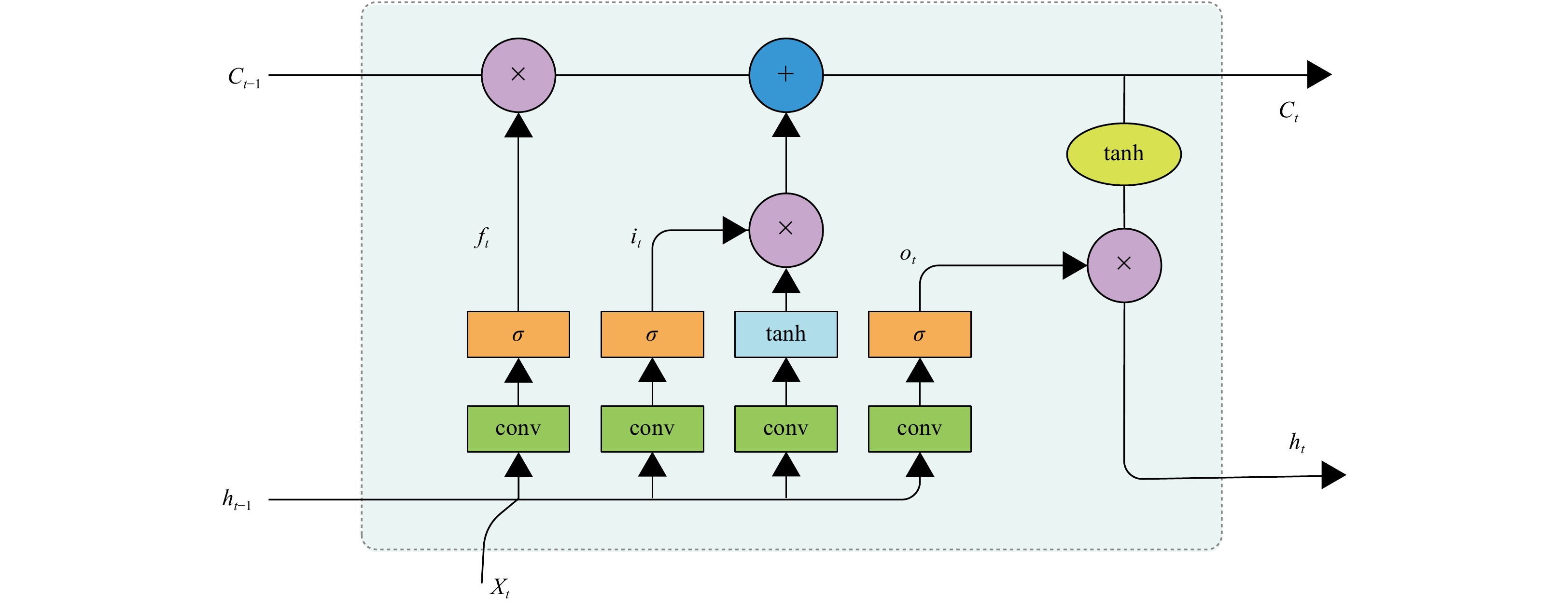
Before introducing ConvLSTM (Fig. 1), it is necessary to recall basic notions of LSTM. It is an improved RNN having a number of memory cells ${C_t}$ (Eq. (1)), each of which has an input gate ${i_t}$ (Eq. (2)), forgetting gate $\,{f_t}$ (Eq. (3)), output gate ${o_t}$ (Eq. (4)) and ${h_t}$ (Eq. (5)). LSTM can preserve meaningful information and remove useless information through the three gates. The input and output of the memory cells are one-dimensional vectors, and LSTM may have multiple memory units named fully connected LSTM. The key equations of LSTM are shown as follows:

Figure  1.  A schematic flow chart of ConvLSTM. “Conv” represents the convolution operation. Spatial information is coded as input in LSTM for tracking temporal evolution. The size of convolutional kenel can be 3×3, 5×5 and 7×7. Multiple kennels are denoted by allows.

DownLoad: Full-Size Img PowerPoint

where “°” denotes the Hadamard product, W and b are the weight matrices of the neural network, $x$ is the input vector, and $\sigma $ is the sigmoid activation function.

ConvLSTM is a variant of LSTM, which embeds convolution operations inside LSTM cells, and it is designed to deal with the problem of spatial-temporal sequence (Shi et al., 2015). ConvLSTM can extract spatial-temporal information through the convolution multiplication. Since convolution kernel has the feature of weight sharing, ConvLSTM network has fewer parameters compared with LSTM network. ConvLSTM equations can be written as follows, where “*” denotes the convolution operator:

2.2 ConvLSTMP3

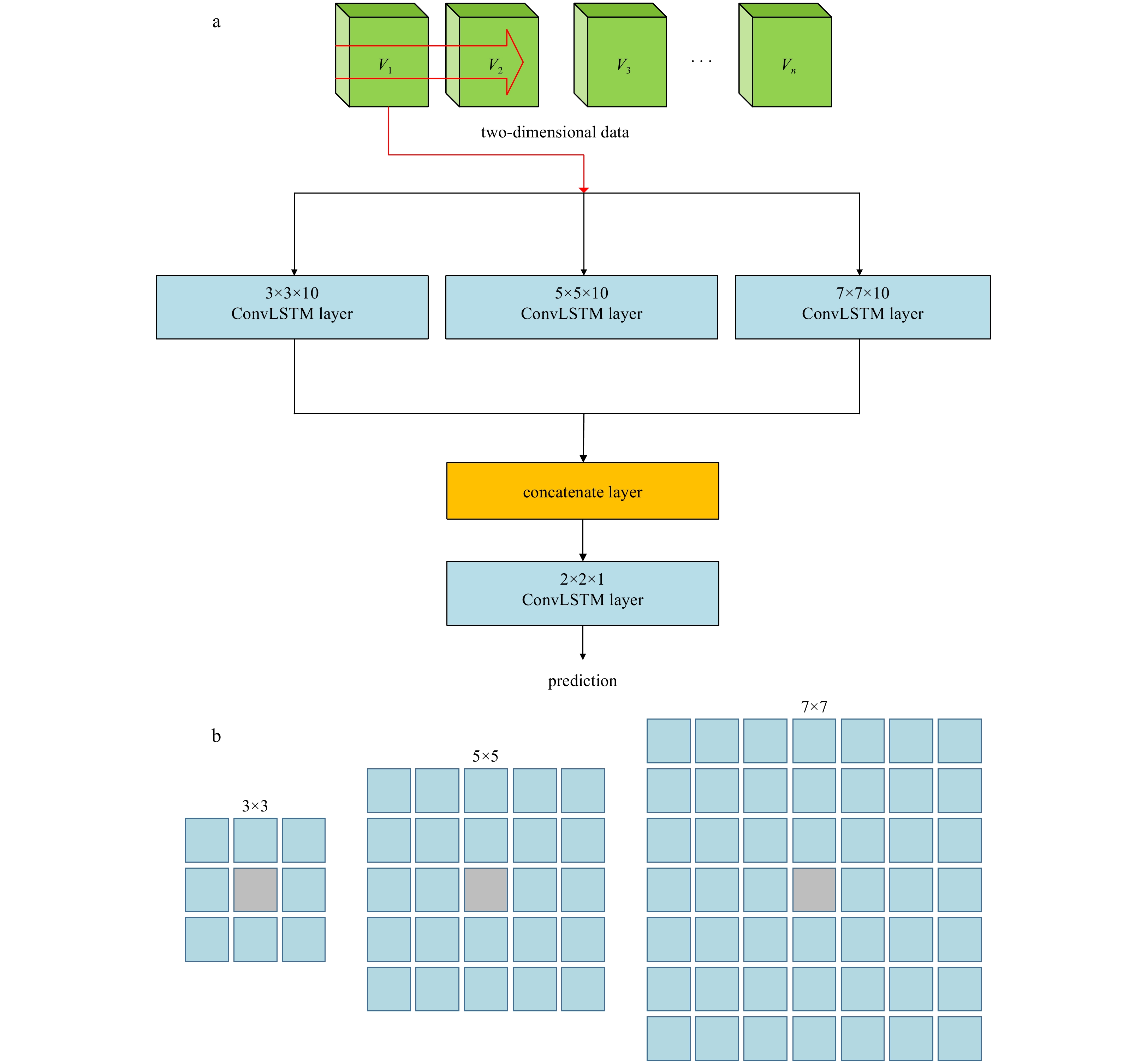
In this study, an improved version of ConvLSTM, named ConvLSTMP3, is developed by parallelizing ConvLSTM model with three sub-network structures. Figure 2a shows the general topological structure of ConvLSTMP3, in which the leftmost, middle and rightmost sub-networks with 10 convolution kennels of size 3×3, 5×5, and 7×7 aim to take the spatial information of the target grid as well as its 8, 24, and 48 adjacent grids (Fig. 2b), respectively. Here the grid is referred to the geographical cell that is formed by the intersection of latitude and longitude. Each sub-network can output 10 feature maps and the information from three subnetworks can be combined from the concatenate layer to produce 30 feature maps. The final 2×2×1 ConvLSTM reduces 30 feature maps of the concatenate layer to one feature map.

Figure  2.  The topologic structure of ConvLSTMP3 (a) and the adjacent grids (blue) of a target grid (gray) corresponding to the convolution kennelsof size 3×3, 5×5, and 7×7 (b). V_i (i=1, 2, …, n) represents datasets that are used to make the i-th-d SSH prediction for a target grid.

DownLoad: Full-Size Img PowerPoint

2.3 ConvLSTM models for comparison

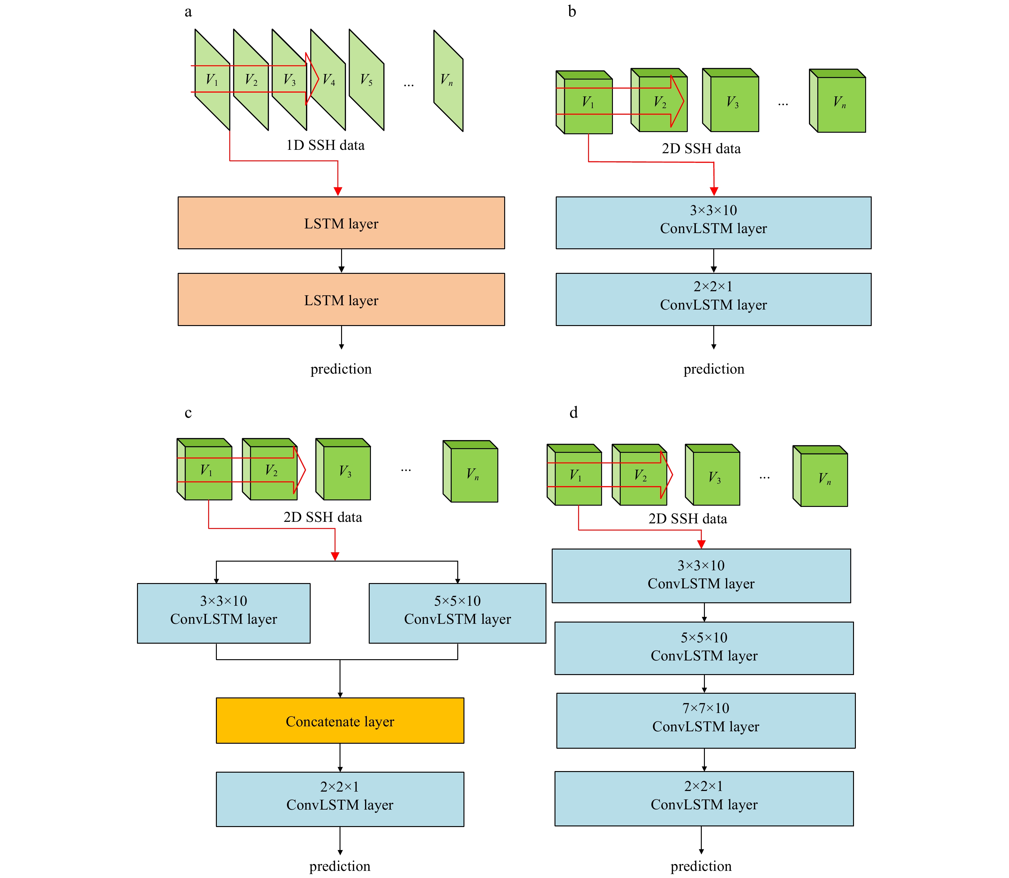
We design extra four ConvLSTM models for comparison with our ConvLSTMP3, denoted as ConvLSTMS1, ConvLSTMP1, ConvLSTMP2 and ConvLSTMS4, respectively, as shown in Figs 3a–d. ConvLSTM is a classical LSTM model with two stacks, which only considers the temporal relationship of data without considering the spatial relationship. With only one path designed, ConvLSTMP1 considers the spatial-temporal relationship of 9 adjacent grids of each grid, while with two sub-networks, ConvLSTMP2 consider both the spatial-temporal relationship between 9 and 25 adjacent grids of each grid. ConvLSTMS4 has the same convolution kernels as ConvLSTMP3 except that the convolution kernels are serially connected.

Figure  3.  The topologic structures of four models: LSTMS1 (a), ConvLSTMP1 (b), ConvLSTMP2 (c) and ConvLSTMS4 (d). V_i (i=1, 2, …, n) represents datasets that are used to make the i-th-d SSH prediction for a target grid. 1D here means only a time series of SSH data on the target grid, while 2D means multiple time series of SSH data on the target grid as well as its adjacent grids.

DownLoad: Full-Size Img PowerPoint

2.4 15-d consecutive prediction

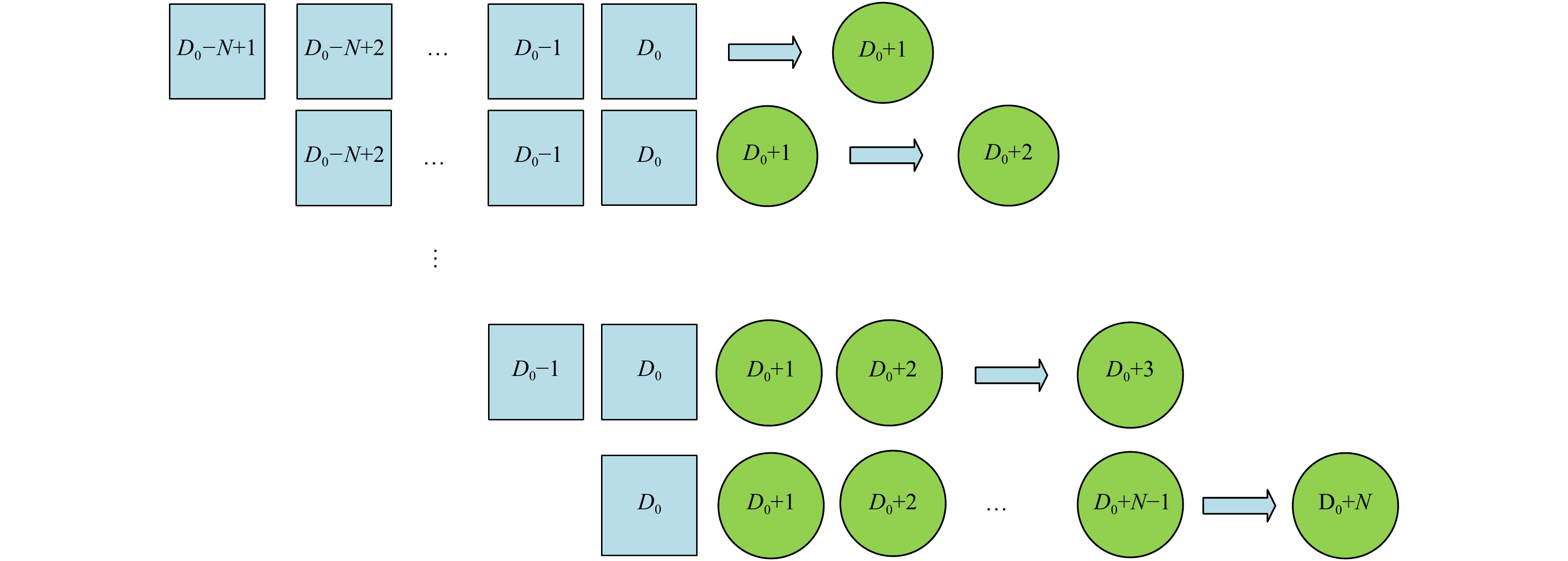
The 15-d consecutive prediction is made by adopting the predicted values as historical values for the input of ConvLSTMP3, as shown in Fig. 4. For a certain grid and a 15-d prediction cycle, the prediction begins with the use of historical SSHs of the last 15 d (i.e., D₀–N+1, D₀–N+2, …, D₀, here N=15 and D₀ denotes the current day) as the input of ConvLSTMP3 to predict the SSHs on the next day (D₀+1). After that, the historical SSHs of the last 14 d (i.e., D₀–N+2, …, D₀, here N=15) and the predicted SSHs on the day (D₀+1) are taken as input of ConvLSTMP3 to predict the SSHs on the day (D₀+2). By repeating this procedure, we can obtain the 15-d SSH prediction on each grid from day (D₀+1) to day (D₀+15). After the 15-d prediction cycle is done, we move to the next prediction cycle by taking (D₀+1) as the current day; as such, we finally obtain the consecutive 15-d SSH prediction for a period from 6 January 2011 to 31 December 2012.

Figure  4.  A schematic diagram illustrating a 15-d prediction cycle. The squares and circles represent the historical SSHs and predicted SSHs, respectively. The squares or circles behind the arrows represent the input of ConvLSTMP3 and the circles ahead the arrows represent the output (prediction). D₀ denotes the current day of the prediction cycle, and N is the length of prediction cycle which is set to 15 (days).

DownLoad: Full-Size Img PowerPoint

2.5 Experimental design

A 5.5°×5.5° region (10.0°–15.5°N, 109.6°–115.1°E, denoted by A) of the SCS located east off Vietnam, is chosen for the deep learning experiments for SSH prediction, as shown in Fig. 5. This region is featured with mesoscale eddies and offshore currents driven by summer monsoon. The daily SSHs in the selected region from the reanalysis dataset of South China Sea (REDOS) (Zeng et al., 2014) from 1 January 1992 to 31 December 2011 with a resolution of (1/10)°×(1/10)° is used for the deep learning, which counts to a sample number of 7 305 (days) in time. With the same resolution as REDOS, the selected region A has a total grid number of 55×56=3 080. Since the baseline of the deep-learning-based SSH prediction method is to deal with the SSH prediction problem as the spatial-temporal series prediction problem, we treat the SSH data of Region A as 7 305 two-dimensional (55×56) matrices or images arranged in temporal order. The SSH data of about 80% days from 1 January 1992 to 1 January 2008 are used to train ConvLSTMP3, 10% days from 2 January 2008 to 1 January 2010 are used for evaluation, and the remaining data of about 10% days from 2 January 2010 to 31 December 2011 are used for testing. In the training process, ConvLSTMP3 is trained by inputting the historical or predicted SSHs of the 15 d to predict the SSHs of the next 15 d. The input data length of 15 d for training ConvLSTMP3, which is the only parameter that LSTM needs to set, is chosen after a set of experiments with different input data lengths, considering the accuracy, efficiency and computation resources. The optimization algorithm of the ConvLSTMP3 employs the Adam algorithm, with the size of each mini-batch being 200. The Adam algorithm is an optimization algorithm commonly used in deep learning, which is able to make the neural network adjust the parameters to the global optimal solution fast. The learning rate is set to 0.001 to control the update ratio of the model. All the experiments are performed on a PC with an I7-8750H processor and 32 GB memory.

Figure  5.  The 5.5°×5.5° region (denoted by A) of the SCS for the deep learning experiments for SSH prediction.

DownLoad: Full-Size Img PowerPoint

3. Results

The root mean squared error (RMSE) and prediction accuracy (ACC) are used to evaluate the prediction skill of different models, which are defined as follows:

where $h_i^{\rm{p}}$ and $h_i^{\rm{t}}$ are the predicted and ground truth values at i-th grid point, respectively, and n is the total number of grid points.

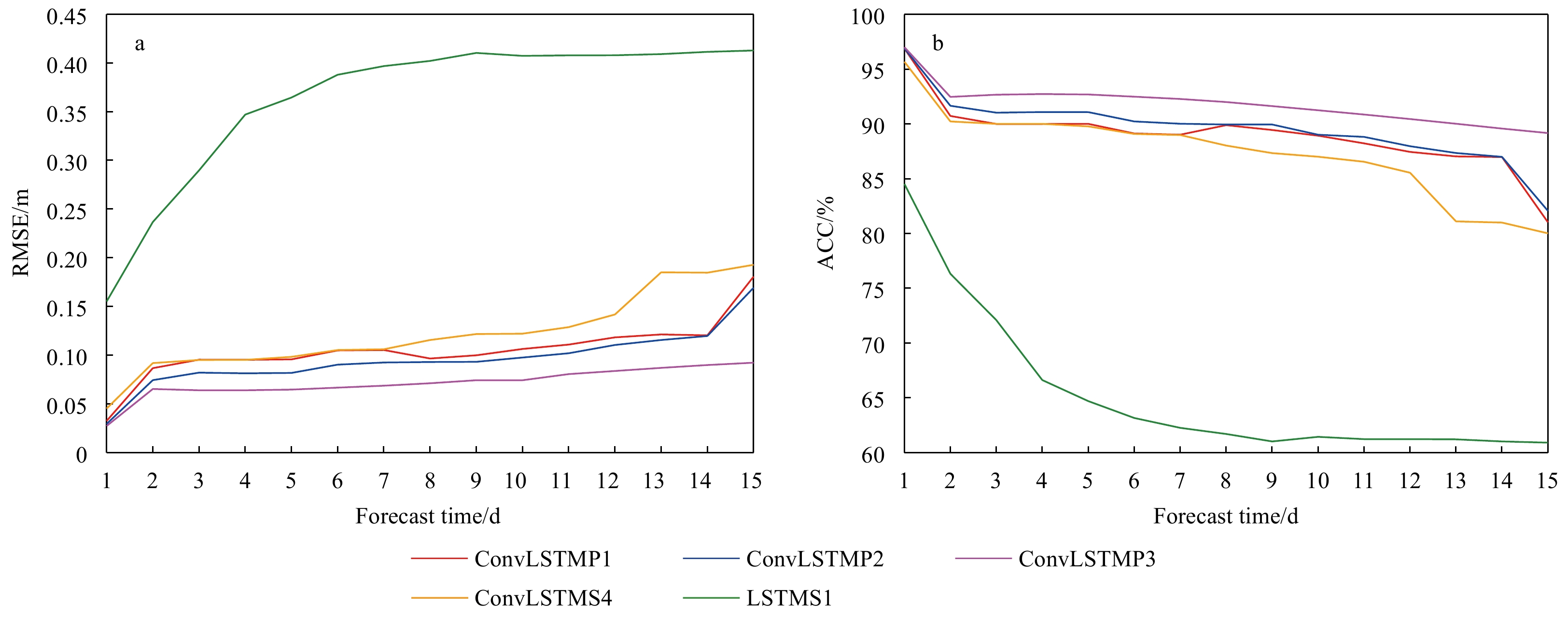
Figure 6 shows the RMSE and ACC of the consecutive 15-d prediction averaged over the testing period from 6 January 2010 to 31 December 2011 from different schemes for Region A. It is obvious that ConvLSTMP3 gives the best performance of the 15-d SSH prediction in comparison with other schemes, with a mean RMSE of 0.057 m and ACC of 93.4% averaged over the 15-d prediction period.

Figure  6.  The RMSE and ACC of the 15-d consecutive prediction averaged over the testing period from 6 January 2010 to 31 December 2011 from different schemes.

DownLoad: Full-Size Img PowerPoint

As an example, we select a summertime period of 1–15 August 2011 to see the performance of ConvLSTMP3 in the prediction of mesoscale eddies and offshore currents in Region A by a comparison with a state-of-the-art dynamical ocean model, i.e., the regional ocean model system (ROMS). ROMS is based on the Navier-Stokes equations and was used to generate the ground truth dataset REDOS by assimilating various observations. To compare the prediction skill of ConvLSTMP3 with that of ROMS, we run ROMS without data assimilation for 15 d starting on 1 August 2011. To be fair, the prediction by ROMS uses the same initial conditions from REDOS as those for ConvLSTMP3 and the same model configuration as those for producing REDOS (Zeng et al., 2015) which covers the entire SCS, while the lateral boundary conditions and the surface forcings (including winds, sensible heat fluxes and latent heat fluxes) are from the same data sources as those for producing REDOS but are climatological mean of August. Figure 7 presents the SSHs from the ground truth and the predictions by ConvLSTMP3 and ROMS, superimposed by the SSH-derived geostrophic currents. The ground truth SSHs show that there is an anticyclonic eddy in the east of Region A which weakened and diminished gradually, whereas a cyclonic eddy developed and intensified in the west of Region A. ConvLSTMP3 well predicts the location and temporal evolution of the two eddies, but slightly underestimates their intensity; ROMS seems to well predict the location and intensity of the two eddies but is not able to predict their temporal evolution. Besides the eddy-related SSHs, ConvLSTMP3 also well predicts the SSH pattern associated with the northeastward offshore currents east off Vietnam coast, but with weaker SSH gradient compared to that from the ground truth and ROMS, which leads to weaker offshore currents. Table 1 gives the RMSE and ACC of the SSH predictions by ConvLSTMP3 and ROMS for the period of 1–15 August 2011. The 15-d-mean RMSE (ACC) of the SSH prediction by ConvLSTMP3 is 0.057 m (93.4%), while that by ROMS is 0.072 m (89.7%), suggesting that ConvLSTMP3 achieves an encouraging prediction skill which is comparable to or even slightly better than that of ROMS. It is worthwhile noting that the computation resource needed for ConvLSTMP3 to make the 15-d prediction is about 100 times less than that for ROMS (Table 2, the CPU cores used for ConvLSTMP3 and ROMS are 1 and 112, respectively), although considerable time (about 32-h CPU time) is needed for the training of ConvLSTMP3 which is similar to the process of building up a full-dynamics ocean model. Therefore, ConvLSTMP3 has great advantage in terms of fast prediction for emergency requirement given that the training is done in advance.

Figure  7.  The ground truth (a–h) and the predicted SSHs by ConvLSTMP3 (i–p) and ROMS (q–x) obtained from August 1 to 15, 2011 in every other day. The black arrows represent the SSH-derived geostrophic currents.

DownLoad: Full-Size Img PowerPoint

Table  1.  The RMSE and ACC of the SSH predictions by ConvLSTMP3 and ROMS during the period of 1–15 August 2011

Period	Item
	RMSE/m			ACC/%
	ConvLSTMP3	ROMS		ConvLSTMP3	ROMS
Day 1	0.028	0.048		96.4	93.4
Day 2	0.017	0.073		98.0	88.6
Day 3	0.027	0.069		96.2	89.5
Day 4	0.033	0.064		96.3	90.2
Day 5	0.039	0.069		95.0	89.5
Day 6	0.051	0.055		93.0	92.3
Day 7	0.049	0.064		93.9	91.1
Day 8	0.049	0.067		93.8	90.4
Day 9	0.067	0.069		91.6	90.4
Day 10	0.055	0.079		93.5	88.4
Day 11	0.066	0.082		92.2	87.7
Day 12	0.083	0.073		89.4	89.8
Day 13	0.076	0.078		90.3	89.0
Day 14	0.085	0.076		89.5	89.6
Day 15	0.077	0.099		91.3	86.0
15-d mean	0.057	0.072		93.4	89.7

 | Show Table

DownLoad: CSV

Table  2.  The configurations of the hardware and software as well as the corresponding CPU time used for the 15-d prediction by ConvLSTMP3 and ROMS

	Hardware configuration	Software configuration	CPU time/s
ConvLSTMP3	Intel (R) Core (TM) I7-8750H (2.2 GHz) processor, 32 GB memory (total number used: 1)	Python 3.6.0	3.695
ROMS	Intel (R) Xeon (R) Gold 6132 (2.60 GHz) processor, 125 GB memory (total number used: 112)	Mvapich2 2.2b	5.451

 | Show Table

DownLoad: CSV

Besides the comparison with ROMS, it is also interesting to compare the performance of ConvLSTM with that of CNN, LSTM and gated recurrent unit (GRU). While LSTM has three gates, GRU has only two gates with fewer parameters and thus requires less computing resource. Considering that the data of spatio-temporal series are three-dimensional, 3D CNN is used for the comparison. As shown in Table 3, LSTM and AGU have similar ACC scores in the SSH prediction that are much lower than those of ConLSTM or CNN, probably due to the fact that both LSTM and GRU consider only one-dimensional time series data in either training or prediction; the performance of 3D CNN is comparable to that of ConvLSTM, but ConvLSTM has slightly higher ACC scores. Given that 3D CNN requires much more computing resources than ConvLSTM, we conclude that ConvLSTM performs the best among these algorithms in the SSH prediction.

Table  3.  The ACC of the SSH predictions by LSTM, GRU, CNN and ConvLSTMP3 during the period of 1–15 August 2011

Periods	Item
	ACC/% (LSTM)	ACC/% (GRU)	ACC/% (3D CNN)	ACC/% (ConvLSTM)
Day 1	84.53	84.77	94.8	96.4
Day 2	76.33	77.33	95.0	98.0
Day 3	72.10	72.20	94.2	96.2
Day 4	66.63	66.67	95.3	96.3
Day 5	64.71	64.71	94.0	95.0
Day 6	63.17	63.23	93.0	93.0
Day 7	62.27	63.01	93.0	93.9
Day 8	61.71	62.00	92.8	93.8
Day 9	61.03	61.07	90.6	91.6
Day 10	61.45	61.55	91.5	93.5
Day 11	61.24	61.43	92.0	92.2
Day 12	61.24	61.24	89.0	89.4
Day 13	61.22	61.21	89.0	90.3
Day 14	61.03	61.05	89.1	89.5
Day 15	60.92	61.00	88.6	91.3
15-d mean	65.30	65.50	92.1	93.4

 | Show Table

DownLoad: CSV

4. Conclusions

A SSH prediction model, called ConvLSTMP3, is developed based on deep learning techniques. The ConvLSTMP3 model can extract spatial information of non-image two-dimensional SSHs by convolution operation and make use of SSH correlation in different spatial extents through three parallel sub-network. The application of ConvLSTMP3 in a region of the SCS using a reanalysis dataset for training and testing indicates that ConvLSTMP3 has a promising skill in the SSH prediction with a 15-d-mean RMSE of 0.057 m and ACC of 93.4% averaged over the testing period of about two years, and it outperforms other deep-learning-based models, including LSTM, GRU and CNN. In particular, ConvLSTMP3 well predicts the spatial patterns and temporal evolution of mesoscale eddies as well as offshore currents in the region of the SCS, and its prediction skill is at least comparable to that of the full-dynamics ocean model ROMS which needs huge amount of computation for the prediction (about 100 times larger than that needed for ConvLSTMP3). Therefore, our study suggests that the deep learning techniques, here referred to as ConvLSTMP3, are very useful and effective in the SSH prediction, and could be an alternative way in the operational prediction of ocean environments in the future, particularly desirable for the emergency needs.