Influences of the Great Whirl on surface chlorophyll a concentration off the Somali Coast in 2017

1. Introduction

The seasonal winds force a seasonal circulation pattern in the Indian Ocean, with a special emphasis on the annual reversals of the Somali Current system (Schott and McCreary, 2001; Schott et al., 2009). During boreal summer, the alongshore southwest winds drive the northward Somali Current and cause coastal upwellings. In the upwelling regions, nutrients enter into the euphotic zone via vertical transport, and boost phytoplankton blooms (Wiggert et al., 2005; Liao et al., 2014). Especially, the cold wedge between 10°N and 12°N off the Somali Coast contributes considerably to the summertime phytoplankton blooms. A large clockwise eddy, Great Whirl (GW), develops near the upwelling wedge with a maximum radius over 200 km, and swirls between 4°N and 10°N for several months (Schott and McCreary, 2001). As a quasi-stationary eddy that survives throughout the Indian summer monsoon, GW continuously transports nutrients brought up by the upwellings to the Arabian Sea, causing a wider range of blooms (Young and Kindle, 1994; Lee et al., 2000; Kawamiya, 2001; Lévy et al., 2007), which make the western Indian Ocean one of the most productive areas in the world’s oceans (Wiggert et al., 2005; McCreary et al., 2009).

GW influences the distribution of sea surface chlorophyll a (Chl a) concentration off the Somali Coast. The Chl a concentration in the ocean surface indicates the quantity and carbon fixation capacity of the main primary producers (Garçon et al., 2001). The characteristics and physical mechanisms of phytoplankton blooms in the Western Indian Ocean were documented in previous studies (Brock et al., 1991; Wiggert et al., 2005). The development of GW has been observed in field (Fischer et al., 1996; Schott et al., 1997), measured by satellites (Beal and Donohue, 2013), and simulated in models (McCreary and Kundu, 1988; Jensen, 1991; Wirth et al., 2002). However, less attention was paid to the ecological effect of GW. Here we focus on the influences of GW on surface Chl a concentration in 2017, a typical case well captured by the satellite ocean color observations. The development of GW in 2017 is a typical case because it is close to the state of multi-year average (figure not shown). Moreover, the ocean color data in study area were less influenced by clouds thus well captured the Chl a concentration variations related with the GW in the time. Through a representative case study, we aim to understand the influences of GW on the spatial distribution of surface Chl a concentration.

Previous studies reached a consensus that mesoscale eddies dominate highly energetic features of global ocean and manifest strong and wide influences on marine biogeochemical processes (Mahadevan, 2014; McGillicuddy, 2016). A considerable part of new productivity in ocean is caused by eddy transport, with an estimate between 10% and 50% (Falkowski et al., 1991; McGillicuddy et al., 1998; Oschlies and Garçon, 1998; Siegel et al., 1999; Letelier et al., 2000; McGillicuddy et al., 2003). Mesoscale eddies regulate the distribution of Chl a concentration not only from the direct advective transport but also from the vertical flux of nutrients and subsequently the growth of phytoplankton (McGillicuddy, 2016). Four kinds of mechanisms were proposed to elucidate the surface Chl a concentration variability affected by eddies, including eddy trapping, eddy stirring, eddy pumping, and eddy-induced Ekman pumping (Siegel et al., 2011; Gaube et al., 2014; McGillicuddy, 2016). Eddy trapping describes that eddy traps fluid from the initial environments in its interiors and maintains a long period (D’Ovidio et al., 2013). Eddy stirring exerts influence where eddy propagates in a Chl a gradient and perturbs the local Chl a gradient via rotation. Eddy pumping, related to the convergence of anticyclone and the divergence of cyclone, can trigger downwelling or upwelling in the interior of eddy. However, eddy pumping is mainly presented during the formation or intensification stage of eddy. Eddy-induced Ekman pumping is attributed to a uniform wind field and applied to a swirling eddy. For anticyclones, the flank of eddy where the current and the wind are in the opposite direction holds higher stress than the other flank. The unequal stress on both flanks of eddy activates upward vertical velocity in the interior of anticyclonic eddy. This effect is opposite to that of eddy pumping.

Based on the satellite data and model outputs, this study aims to investigate the temporal evolution and spatial distribution of Chl a concentration in response to GW, which is important to understand physical-biological-biogeochemical interactions.

2. Data and methods

Multi-satellites merged sea surface height (SSH) anomaly data were obtained from the Archiving, Validation and Interpretation of Satellite Oceanographic data (AVISO) (Pujol et al., 2016). The altimeter product was produced and distributed by the Copernicus Marine and Environment Monitoring Service, based on measurements from TOPEX/Poseidon, Jason-1, Jason-2, ERS-1, ERS-2, and ENVISAT. The daily 0.25° gridded data were used to identify and characterize the GW. The Mesoscale Eddy Trajectory Atlas proposed by Chelton et al. (2011) was used to collect basic physical information of GW, including start time, end time, radius, amplitude, speed, and spatial position. According to the automated identification procedure, eddy is identified by the outermost contour line of the SSH field that meets the maximum geostrophic speed and closed contour simultaneously. Radius (R) is defined as the radius of a circle whose area is equal to that enclosed by the contour of the maximum circum-average speed. Amplitude is the height difference between the maximum of SSH in eddy centroid and that on the contour defining the eddy periphery. Speed is defined as the average speed of the contour defining the eddy radius.

The cross-calibrated multi-platform (CCMP) ocean vector wind analysis is a 0.25°, 6 h, global product created by a variational analysis method (VAM). The input data are a combination of inter-calibrated satellite data from numerous radiometers and scatterometers and in-situ data from moored buoys (Atlas et al., 2011). The relative velocity field of wind over surface current was used to calculate the vertical velocities induced by eddy-induced Ekman pumping (WEP) (Halpern, 2002; Risien and Chelton, 2008; Renault et al., 2012):

where ${\rho _{_{\rm{W}}}}$ is the sea water density, $\,f$ is the Coriolis parameter, $\,\beta $ is the Coriolis parameter gradient, $\tau $ is wind stress for the relative wind fields, and ${\tau _x}$ is the zonal wind stress.

The sea surface Chl a concentrations, which were processed using SeaDAS software (Version 7.5) from MODIS Aqua data, have a spatial resolution of 1 km and a temporal resolution of 8 days. Data for 8 d intervals were chosen because they were less masked by clouds and the Chl a blooms were well recorded by satellite in 2017.

The high-resolution operational mercator global ocean analysis and forecast product, which is produced by version 3.1 of the Nucleus for European Modelling of the Ocean (NEMO) and provided by Copernicus Marine Environment Monitoring Service (Madec, 2008), were used to explore the vertical structure of GW. NEMO 3.1 is a primitive equation, Boussinesq approximation ocean model with a configuration of tripolar ORCA12 grid type (Madec and Imbard, 1996). The global ocean output files are displayed with a 0.125° horizontal resolution with a regular longitude/latitude equirectangular projection. Fifty vertical levels are ranging from 0 m to 5 500 m at an unequally spaced scale. The product contains three-dimensional salinity, potential temperature, current from top to bottom, and two-dimensional sea surface level and mixed layer thickness. Figure 1 shows the SSH provided by the model product and the sea level anomaly provided by AVISO database at the same time from June to November. The consistent similarity between SSH from the model and the satellite observations suggests that GW could be well reproduced by the model, especially in terms of large-scale features. Therefore, this global ocean analysis and forecast product can be used to investigate the evolution of GW.

Figure  1.  Comparison of surface patterns between the sea surface height (SSH) from satellite observations (black solid contours for SSH anomaly (SSHa) > 0 and black dash contours for SSHa < 0) and the SSH from model products (colors) at different time.

DownLoad: Full-Size Img PowerPoint

In this study, composite analysis was used to analyze the mechanisms on how GW influences the local biogeochemical processes. Given that the size and shape of eddy varies every day, the eddy radius was normalized by R first. For the daily dataset, a standard circular area with a radius of 2R from the eddy center was established and projected onto a uniform square grid with a spatial scale from –2R to 2R. We then uniformly interpolated the distribution information of Chl a concentration anomaly in the eddy on a R scale. Finally, we composited all the normalized eddy snapshots of Chl a concentration anomaly to access the mean spatial distribution of Chl a concentration anomaly in different months.

3. Results and discussion

3.1 General features of GW in 2017

GW is a clockwise circulation near the Somali Coast and its surface velocity can reach approximately 1 m/s (Fig. 2). GW was originally generated at 7°N, 53°E on June 13, 2017. After the formation, GW continued to move northward (Fig. 2) in the initial development stage. From mid-July to mid-August, the amplitude of GW rapidly increased to the maximum (Fig. 3b), and the propagating speed also reached the maximum. Moreover, the spatial structure of eddy became a regular ellipse. During the decay phase, the shape of GW distorted strongly. GW finally disappeared at 9°N, 52°E on November 12 with a total duration of 153 d.

Figure  2.  Location of Great Whirl centers (colored dots) in June-November 2017 and the surface currents (vectors) on August 20, 2017. The red, brown, and blue enclosed lines represent the area of GW in June, August, and November respectively.

DownLoad: Full-Size Img PowerPoint

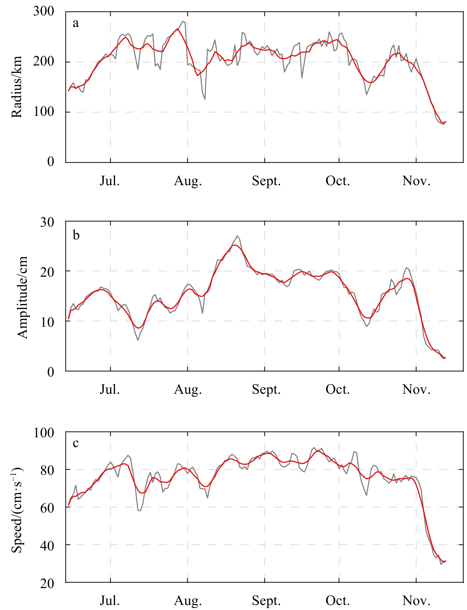
Figure  3.  Time evolution of the radius (a), amplitude (b) and speed (c) of GW in 2017. The grey lines represent the original results, and the red lines represent the results that are smoothed using a 7-point moving average filter.

DownLoad: Full-Size Img PowerPoint

Figure 3 shows the time evolution of the GW’s radius, amplitude, and speed. The evolution can be divided into three stages: growth phase, maturity phase, and decay phase. The radius, amplitude, and speed all grew from mid-June, entered plateau between late August to early September, and decayed rapidly after. The radius of GW increased dramatically after it formed on June 13, exceeding 250 km in late July after a short period of fluctuation. In the next two months, the radius remained about 200 km. Since then, the radius decreased to less than 100 km until it disappeared in November. Throughout its life cycle, the average radius is 205 km. The radius of the GW can be affected by compressing or merging with the surrounding eddies. In general, the surrounding eddies have two sources: cyclonic eddies shed from the northern upwelling region, which rotate clockwisely around GW (Melzer et al., 2019); and eddy generated as a dynamical response to internal instability, which propagate westward to approach GW (Jensen, 1991). The amplitude of the eddy represents the SSH anomaly caused by the eddy, which represents the evolution of GW intensity. The amplitude increased at a fast rate and reached the peak of 27 cm on August 20. The amplitude then decreased slowly within two months and decreased rapidly in early November. The average amplitude of GW in 2017 is 16 cm, which is larger than the average amplitude of global mesoscale eddies, 7 cm (Chelton et al., 2011). The trend of speed change is similar to the amplitude and reached the peak of 92 cm/s on September 20.

Figure 4 shows the north-south velocity along the zonal section of GW at different times. On June 20, 7 d after the formation, the depth of GW was close to 800 m consistent with a numerical study proposed by Jensen (1991), in which study anticyclonic motion could be seen at 850 m depth after 18 d of formation. From June to July, the radius of GW increased, but its vertical depth did not change considerably, because the amplitudes of GW were similar at the two periods. In mid-August, the amplitude reached the maximum, with vertical penetration to 800 m. From October, the vertical depth of GW continued to decrease, and the GW finally disappeared in November.

Figure  4.  Vertical section of north-south velocity across the center of Great Whirl at different time from model products. The white lines represent the mixed layer depth.

DownLoad: Full-Size Img PowerPoint

3.2 Impact on surface Chl a concentration

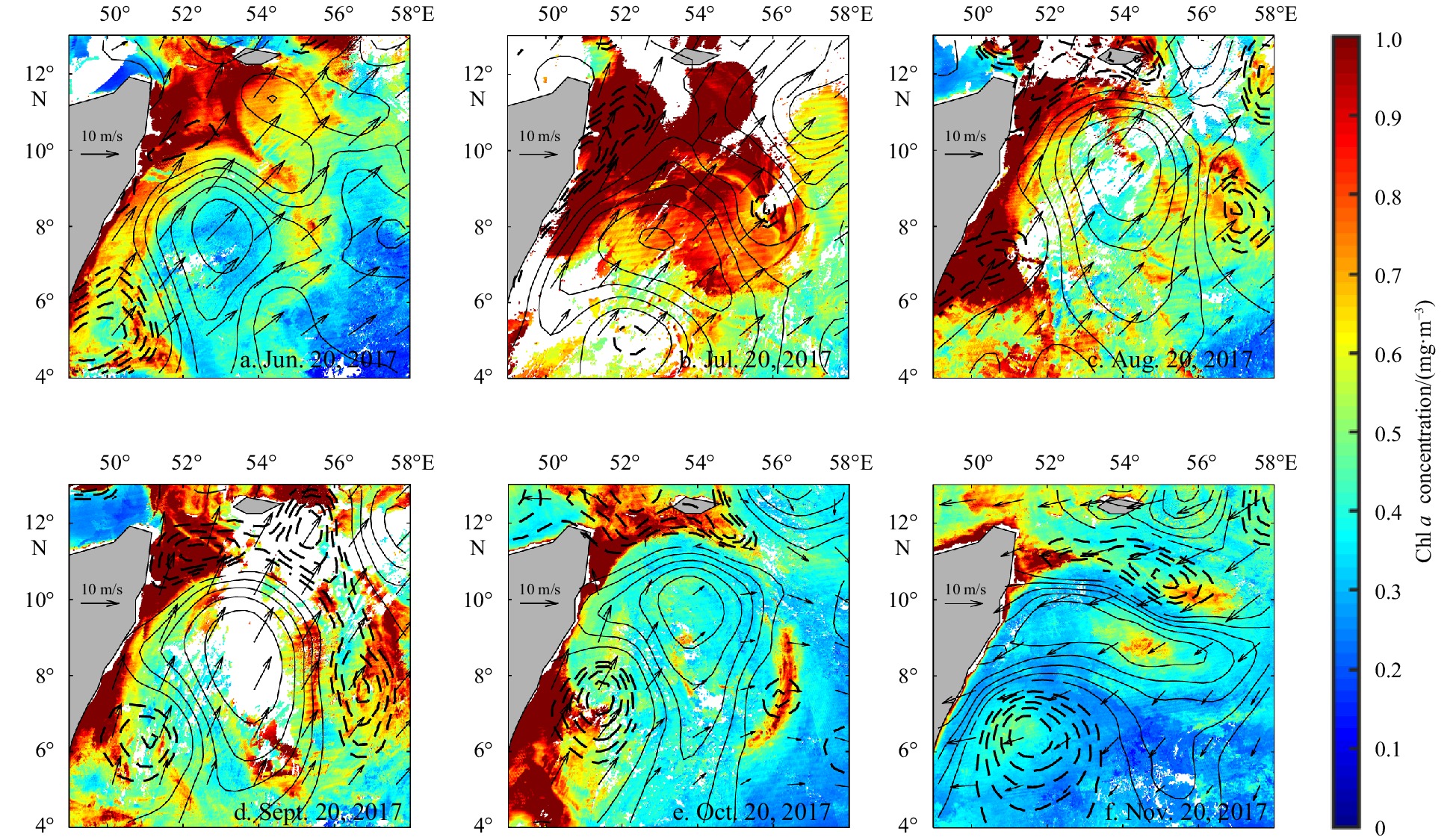
With the onset of summer monsoon, southwesterly winds induced coastal upwelling, uplifting the nutricline, causing nutrient enrichment in the upper ocean and triggering the phytoplankton blooms, as manifested in the coastal and wedge-shaped upwelling areas (Fig. 5a). Then GW transported nutrients to a wider area, spreading water containing rich phytoplankton and nutrients eastward to the Arabian Sea, and causing a wider range of phytoplankton blooms (Figs 5b-d). Water with high Chl a concentration even entered the interior of GW in July (Fig. 5b). At the end of the summer monsoon, the Somali Current started to reverse and the coastal upwelling gradually disappeared (Figs 5e-f).

Figure  5.  Chl a concentration distribution around the Great Whirl in 2017. The SSH anomaly is from satellite observations (black solid contours for SSHa>0 and black dash contours for SSHa<0). The colors represent Chl a concentration. The vectors represent the cross-calibrated multi-platform surface winds.

DownLoad: Full-Size Img PowerPoint

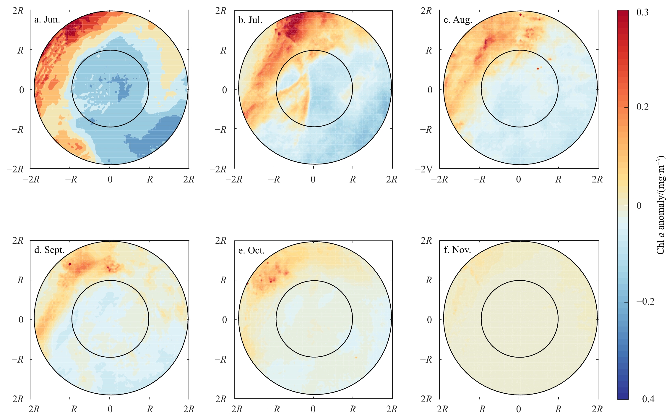
To study the response of distribution of Chl a concentration to GW, we used a composite analysis to construct the spatial structure of Chl a concentration anomalies in different months in the life cycle of GW (Fig. 6). The spatial structures of sea surface Chl a concentration varied in different months. From June to October, all the spatial structures of Chl a concentration anomaly were dipolar in the 2R region, with one positive core in the northwest of GW, due to the high background Chl a concentration gradients caused by the coastal upwelling. Eddy stirring also facilitated the formation of the dipole pattern. In November, when the summertime phytoplankton blooms came to an end, the homogeneous distributions of Chl a occupied the research area.

Figure  6.  Composite averages of Chl a concentration anomaly for every month in the life cycle of Great Whirl. Panels a to f correspond to June to November respectively.

DownLoad: Full-Size Img PowerPoint

The Chl a concentration anomaly in the anticyclonic eddy area controlled by eddy pumping is expected to be dominated by a negative core. The distribution of Chl a concentration from June to September displayed negative cores clearly in the 1R region, but rather uniform in October and November. In October, high Chl a concentration anomaly in the northwest of eddy indicated that the upwelling still existed. The non-negative core in the 1R region means that the Chl a concentration in GW was relatively high in October, which was supported by the time series of Chl a concentration (Fig. 7a). In November, with the establishment of the northeast monsoon, the costal upwellings decayed gradually, and the distribution of Chl a concentration in the sea surface tended to be uniform. Although the spatial structure of Chl a concentration anomaly in July was dominated by the negative core in the 1R region, some positive values existed. Chl a concentration in the GW also reached the maximum in July (Fig. 7a).

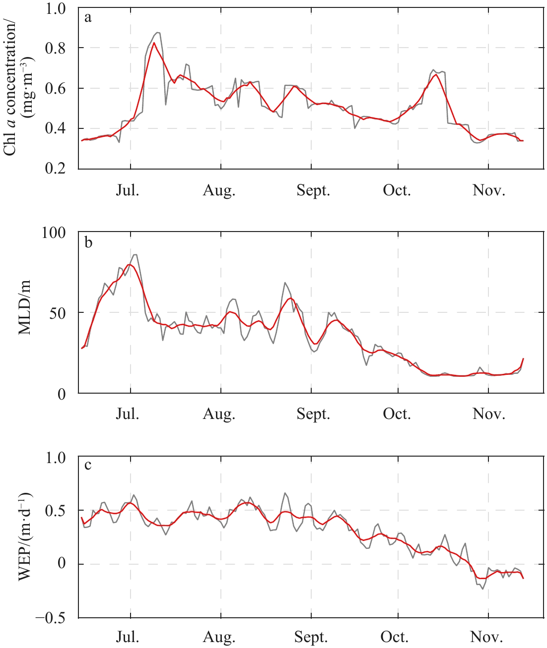
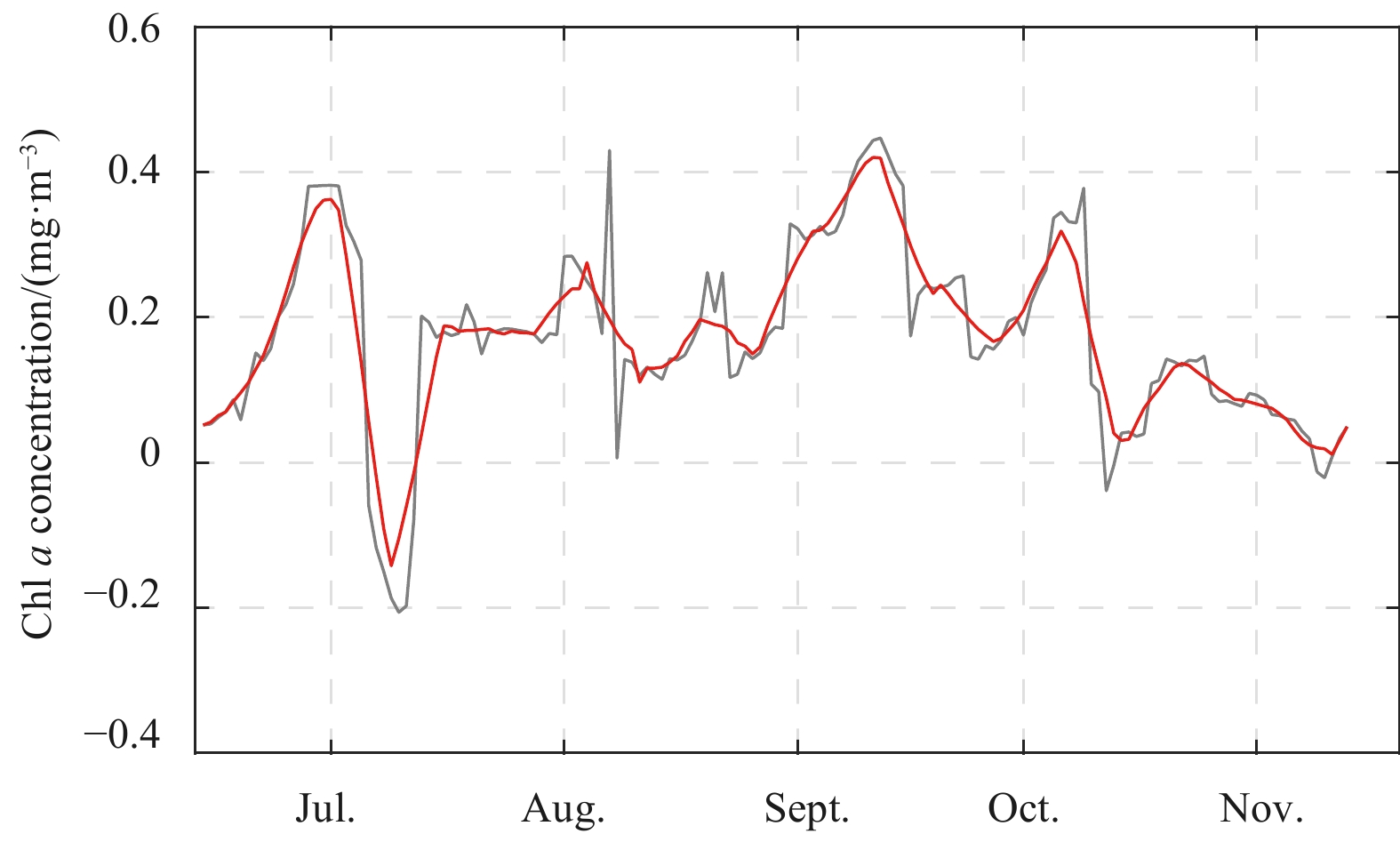
Figure  7.  Time evolution of the Chl a concentration (a), mixed layer depth (MLD) (b) and vertical velocities induced by eddy-induced Ekman pumping (WEP) (c) of Great Whirl in 2017. All the three parameters in GW are defined as the mean value within 0.5R. The grey lines represent the original results, and the red lines represent the results that are smoothed using a 7-point moving average filter.

DownLoad: Full-Size Img PowerPoint

Figure 7a shows the time evolution of the mean concentration of Chl a in the interior of GW in 2017. The Chl a concentration in the interior of eddy is defined as the mean concentration of Chl a within 0.5R. The Chl a concentration was relatively low during the GW formation stage, and then the concentration increased rapidly and reached a peak in July, and then gradually decreased (Fig. 7a). The second peak occurred in October, after which the concentration rapidly decreased (Fig. 7a).

These findings show the spatial distribution of Chl a concentration in GW and quantifies its response. Nevertheless, the main mechanism of GW in affecting the Chl a concentration distribution remains unknown. Off the Somali Coast, the growth of phytoplankton is not limited by light, but the nutrients are the main limiting factors (Brock et al., 1991; Wiggert et al., 2005; Lévy et al., 2007; Liao et al., 2016). In the interior of GW, the mixed layer depth (MLD) and the Chl a concentration decreased after July, implying potential connections between them.

The MLD in the north Indian Ocean has a semi-annual cycle. From December to February of the following year and from June to August, the MLD peaked twice (Kara et al., 2003). The tendency of the MLD in GW was basically consistent with the seasonal change of background in 2017 (Fig. 7b). The MLD in GW reached its maximum in early July and then declined. From mid-July to late August, the MLD was in a relative steady phase. From the beginning of September, the MLD decreased gradually until it disappeared. On one hand, in the anticyclone growth stage, eddy pumping can deepen the mixed layer. Under the combined effect of eddy pumping and the monsoon in July, the mixed layer reached the deepest level, enriching the nutrients in the upper ocean and causing Chl a blooms. On the other hand, eddy pumping causes a downward movement of the ocean surface, which can lead to Chl a depression in the interior of an anticyclone (McGillicuddy et al., 1998). The deepening of the mixed layer in later June facilitated the phytoplankton blooms in early July. Besides, the advection of Chl a from the cold wedge into the GW also contributed to the Chl a peak in July.

In general, uniform winds flowing over an anticyclonic eddy can produce upwelling in the interior of the eddy. Eddy-induced Ekman pumping is expected to lead to positive Chl a concentration anomalies in anticyclone eddies. It engenders relatively smaller upward vertical velocities than eddy pumping, but works in the whole lifetime of eddy (Gaube et al., 2014). During the summer monsoon, the vertical velocity caused by the eddy-induced Ekman pumping reached 0.6 m/d in June, and then it decreased from September. In particular, the upwelling persisted from June to late October, transporting nutrients from the deep layer to the upper layer, hence facilitating the increase of Chl a concentration in GW. Thus, eddy-induced Ekman pumping might be one factor to promote the Chl a blooms in early July. However, the effect is not obvious during the whole lifetime of GW. The eddy-pumping effect caused by GW possibly counteracted the effect of eddy-induced Ekman pumping.

Eddy trapping may also be a mechanism for the increase in Chl a concentration inside an anticyclone eddy. However, we noticed that the Chl a concentration inside the GW was low when the initial GW formed, so eddy trapping was not the reason to cause Chl a blooms in early July. Considering that the GW is a quasi-stationary eddy spinning in a limited area, both eddy stirring and eddy trapping are not important.

After the formation of GW, the Chl a concentration in the interior of GW had a declining trend, except for the blooms in early July and mid-October. In July, the Chl a from the cold wedge penetrated into the interior of GW by horizontal transportation. Under the monsoon forcing, the deepening of the mixed layer boosted the increase of nutrients in the upper ocean and the eddy pumping further maintained the tendency. Moreover, eddy-induced Ekman pumping transported nutrients to the upper ocean continuously. Hence, the Chl a blooms in the interior of GW might be caused by the combined effect of eddy horizontal advection, mixed layer deepening, and eddy-induced Ekman pumping in early July. When the October blooms occurred, the MLD and vertical velocity of eddy-induced Ekman pumping were at low levels. In particular, the radius, amplitude, and speed of GW decreased rapidly, indicating the reduced intensity of GW at that time. The weak eddy intensity means more frequent water exchange across the edge of eddy, so that the external nutrient-rich water is more likely to enter the interior. The blooms in October was probably attributed to the weak intensity of GW, thus, the Chl a was enriched in the interior of GW by water exchange.

To better understand the effect of GW on the distribution of Chl a concentration in the surface layer, we calculated the averaged concentration differences in Chl a between the interior and periphery of GW (Fig. 8). The averaged concentration in the interior of GW is defined as the mean concentration of Chl a within 0.5R of GW, while GW’s periphery is defined as the mean value between 1R and 2R. The concentration at the GW’s periphery is generally greater than the value in interior of GW, except in early July. The correlation coefficient between the Chl a differences and eddy amplitude is 0.44 (p<0.01), suggesting that the eddy intensity could influence the distribution of Chl a concentration on the sea surface, and then affect the local ecology (Mahadevan, 2014).

Figure  8.  Time evolution of differences between Chl a concentration in the interior and periphery of the Great Whirl. The parameter in the interior of Great Whirl is similar to that in Fig. 7. Accordingly, the parameter at the periphery is defined as the mean value of Chl a concentration between 1R and 2R. The grey lines represent the original results, and the red lines represent the results that are smoothed using a 7-point moving average filter.

DownLoad: Full-Size Img PowerPoint

4. Conclusions

The satellite observations captured the general characteristics of GW and its influence on Chl a in 2017. GW first appeared at 7°N, 53°E on June 13, 2017, moved northward and disappeared at 9°N, 52°E after 153 d. The average radius of GW is 205 km and the average SSH amplitude is 16 cm.

The influence of GW on Chl a was investigated. With the onset of summer monsoon, southwesterly winds induced coastal upwelling and triggered phytoplankton blooms in the coastal areas. Moreover, GW transported nutrients eastward to the Arabian Sea, causing a wider range of phytoplankton blooms. We used the composite analysis to study the response of distribution of Chl a concentration to GW. In the growth and mature phases of GW, the Chl a concentration anomaly in the eddy area (1R) was dominated by a negative core. The 2R region showed a dipolar pattern, which was caused by the strong coastal upwelling. The time evolution of the mean concentration of Chl a in the interior of GW was also estimated. The Chl a concentration decreased during the lifetime of GW, except in early July and mid-October. Eddy horizontal transportation, the deepening of the mixed layer caused by monsoon and eddy pumping, and the upward transportation of nutrients caused by eddy-induced Ekman pumping, all contributed to the blooms in early July (Fig. 9a). In October, the blooms in the interior of GW were probably due to the suddenly weakened intensity of eddy, which facilitated water exchange at the edge of GW. The ocean processes occurred at the edge would import phytoplankton into the interior of GW (Fig. 9b).

Figure  9.  Schematic diagram of GW and the underlying mechanisms of the Chl a bloom in July (a) and October (b). R and A are the radius and SSH amplitude of GW respectively. The spatial distribution of Chl a concentration was monthly averaged. The mixed layer depth and the vertical velocity of eddy-induced Ekman pumping were calculated by monthly averaged in 0.5R of GW.

DownLoad: Full-Size Img PowerPoint

Although we selected the year 2017 with available Chl a satellite observations as much as possible, the cloud cover was still inevitable in the ocean color remote sensing, thereby causing inaccuracies in calculating our results. More in situ observations are necessary to investigate this region in the future.

Acknowledgements

We thank the Big Earth Data Repository for the sea surface chlorophyll a concentration data (http://repository.casearth.cn/), AVISO database for the SSH anomaly and Mesoscale Eddy Trajectory Atlas (https://www.aviso.altimetry.fr/en/home.html), CCMP for the ocean vector wind (https://climatedataguide.ucar.edu/climate-data/ccmp-cross-calibrated-multi-platform-wind-vector-analysis), and CMEMS for the analysis and forecast product (https://resources.marine.copernicus.eu/).