Figure
1.
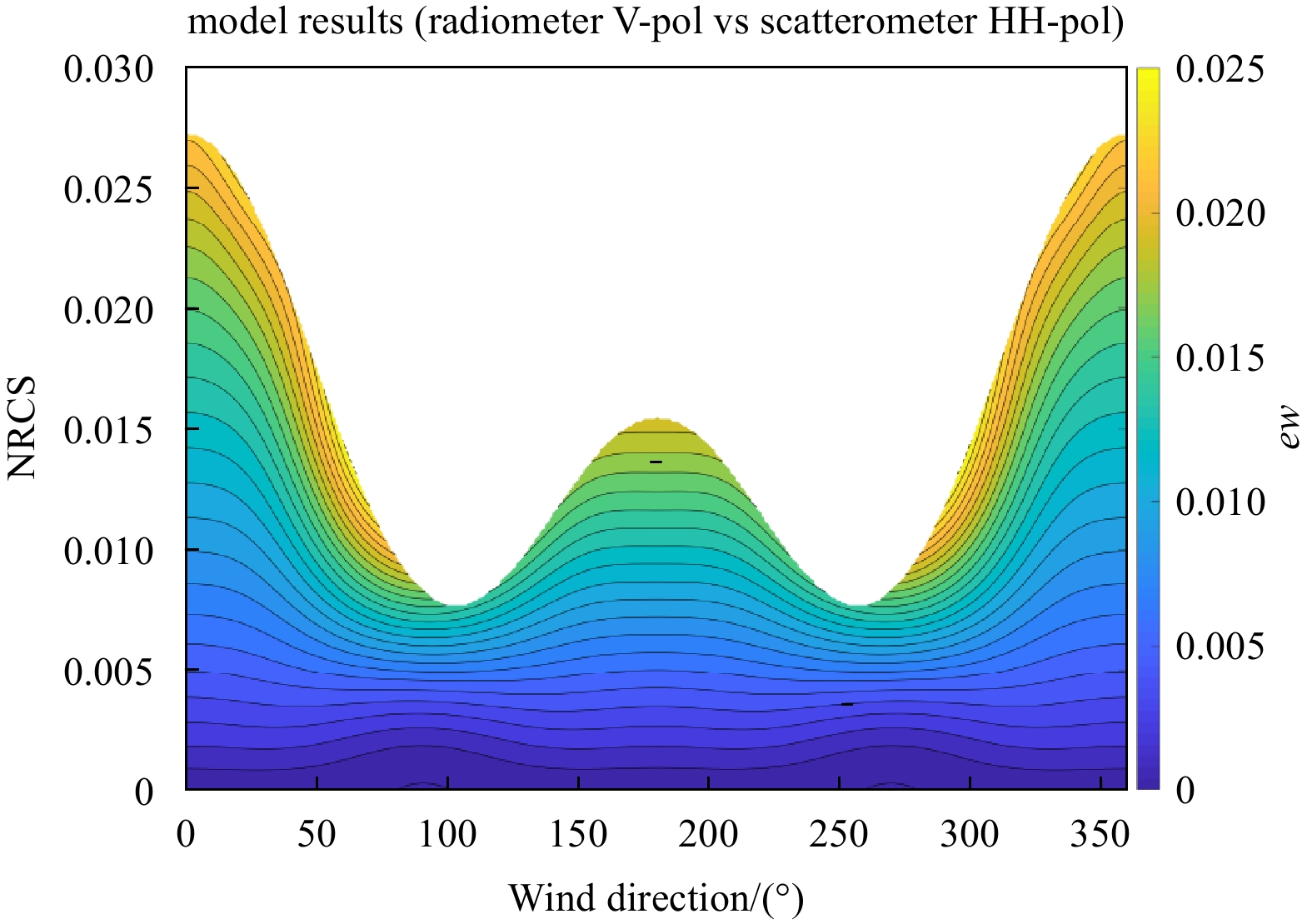
Wind-induced emissivity versus NRCS and wind directions (beam-3, incidence angle of 46.29°, wind direction bins of 10°, and NRCS bins of 0.001).
| Citation: | Wentao Ma, Guihong Liu, Yang Yu, Yanlei Du. Roughness correction method for salinity remote sensing using combined active/passive observations[J]. Acta Oceanologica Sinica, 2021, 40(11): 189-195. doi: 10.1007/s13131-021-1744-z

|
Sea surface salinity (SSS) plays a significant role in energy exchange between the ocean and atmosphere as well as tracking the global water cycle (Reul et al., 2020). The Aquarius/SAC-D satellite-carrying combined L-band active/passive instruments was designed to measure global SSS. The Aquarius mission aims to provide the science community with monthly SSS maps at a 150 km spatial scale and an accuracy of 0.2 (Lagerloef et al., 2008). To achieve the required accuracy in SSS measurements from L-band radiometers, it is very crucial to accurately correct the radiation that is emitted from the ocean surface induced by the impact of sea surface roughness (Yueh et al., 2001).
This roughness signal must be removed from the Aquarius observations to obtain the emissivity of a specular ocean surface. Ocean roughnesses, including large-scale gravity waves, small-scale capillary waves and foam, are mainly induced by surface winds. To improve the performance of removing the surface roughness emissivity signal from radiometer measurements, an L-band scatterometer is also equipped on the Aquarius/SAC-D satellite to simultaneously detect the ocean wind field (Yueh et al., 2013). The merits of the combination of active and passive instruments are that the active radar observations can provide a simultaneous description of the surface roughness, which is significantly useful for removing the roughness signal from the passive emissivity signal (Isoguchi and Shimada, 2009; Yueh et al., 2010).
Numerous studies based on various instruments and observation techniques have been performed to derive the empirical geophysical model function (GMF) for the wind-induced surface emissivity signal, which is also known as excess emissivity. The first formulation of the L-band emissivity as a function of wind speed was proposed by Hollinger (1971), in which the data provided by a microwave radiometer mounted on a fixed ocean platformwas used. Subsequent studies and experiments include the two-scale scattering model (Dinnat et al., 2003), the Wind and Salinity Experiment (WISE), which was part of the pre-launch campaign for Soil Moisture and Ocean Salinity (SMOS) (Camps et al., 2004; Etcheto et al., 2004), and the airborne Passive-Active L-band Sensor (PALS), which was part of the Aquarius pre-launch efforts (Yueh et al., 2010). More recently, the L-band emissivity was analyzed using brightness-temperature observations from the SMOS sensor (Guimbard et al., 2012; Yin et al., 2012, 2016) and for the Aquarius instrument using the combined active-passive (CAP) approach (Fore et al., 2014). Several L-band emissivity model functions based on preliminary data analyses have been presented by Meissner et al., (2012a, 2018), Meissner and Wentz (2012). However, for the Aquarius/SAC-D mission, in previous salinity retrieval algorithms, the roughness-induced brightness temperatures are corrected using the wind field retrieved from the H-polarization brightness temperature and HH-polarization normalized radar cross-sections (NRCSs) (Ma et al., 2014; Meissner et al., 2018). Considering that both the scatterometer NRCS and radiometer brightness temperature (TB) are observations from the sea surface, better roughness correction results would result if the relationship between the sea surface TB affected by the sea surface roughness and the scatterometer NRCS can be directly established.
The rest of this paper is organized as follows. In Section 2, the data used in this studyis briefly described. In Section 3, the relationship between brightness temperature and normalized radar backscatter cross-section (NRCS) is shown. In Section 4, the validation of the new model is given. A summary is given in Section 5.
The Aquarius end-of-mission (Version 5, abbreviated as V5.0) salinity dataset was released in December 2017. The Aquarius V5.0 datasets are described and discoverable via the data portal of the Physical Oceanography Distributed Active Archive Center (PO.DAAC). The Aquarius Level-2 (including science data in swath coordinates and matching ancillary data) data are used in this study. The sea surface TB and NRCS collected and collocated in the dataset are extracted for this research. The incidence angles of Aquarius are 29.36°, 38.49°, and 46.29°, which correspond to beam-1, -2, and -3, respectively (Meissner et al., 2018).
Ancillary data integrated in the datasets are also used in this study. The source of the ancillary sea surface temperature (SST) is the daily gridded high-resolution sea surface temperature (GHRSST) field of level 4 from the Canadian Meteorological Center (CMC). The CMC field is linearly interpolated in space and time to the boresight location of the Aquarius observation. The reference SSS field is the analyzed monthly Scripps ARGO SSS product. The computation of flat sea surface TB is based on the Fresnel equations, Meissner-Wentz model of seawater permittivity (2004, with the 2012 update) (Meissner and Wentz, 2004, 2012), and the ancillary SST field from the CMC. The NCEP GDAS 1-deg, 6-h scalar wind-speed field is used as the background field in the surface roughness correction and the Aquarius wind-speed retrievals (Meissner et al., 2014). It is linearly interpolated in space and time to the boresight location of the Aquarius observation.
The data from September to December 2011 is used for model development. Approximately 3.81 million data points (more than 1.25 million for each beam) are used. Particularly, the data with land contamination larger than 1% or with rainfall is discarded from the dataset. The data from January to March 2012 was used for model validation. For each beam, the number of data points are approximately 900 000.
In previous salinity retrieval algorithms, the roughness-induced TBs are corrected using the wind fields retrieved from the H-polarization TB and HH-polarization NRCSs (Ma et al., 2014; Meissner et al., 2018). However, using a 10-m high wind speed as the intermediate variable for sea surface roughness correction may result in large errors. First, the wind-speed retrieval accuracy is easily affected by atmospheric stability and the accuracy of auxiliary data (Yueh et al., 2013; Fore et al., 2014). Second, more model errors may be introduced in the process of wind-speed retrieval and further calculations of TB. Considering that both the scatterometer NRCS and radiometer TB are observations from the sea surface, better roughness correction results would result if the relationship between the sea surface TB affected by the sea surface roughness and the scatterometer NRCS can be directly established.
In the model-building process, to eliminate the influence of other parameters, it is necessary to subtract the quiet sea surface TB from the total sea surface TB. Then, the excess TB of wind would be obtained. The quiet sea surface TB is calculated on the basis of the Meissner-Wentz (2004, with the 2012 update) (Meissner and Wentz, 2004, 2012) dielectric-constant model of seawater using the SST, SSS, and several other auxiliary parameters. The rough sea surface wind-induced excess emissivity (ew) is defined as the ratio of the excess TB over the SST, i.e.,
| $$ e{w_{p'}} = \frac{{{{\rm{TB}}_{p'}} - {{\rm{TB}}_{{\rm{flat}},p'}}}}{{{\rm{SST}}}}, $$ | (1) |
where the ew is considered to be only related to the sea surface wind speed and wind direction in this study. The subscript flat represents the calm sea surface and p′ represents horizontal polarization (H-pol) or vertical polarization (V-pol). Similarly, the NRCS observed by the scatterometer is also supposed to be related only to the sea surface wind speed and wind direction in previous studies (Yueh et al., 2013). Then, the relationship between ew and NRCS can be established directly. In the Aquarius dataset, the NRCS has been transformed into dB scale, but in this work the computations are performed based on the NRCS in linear scale, which can be restored from the dB scale as follows:
| $$ {\sigma _{pp}} = 10^ {\left({{\rm{NRCS}}/10} \right)}, $$ | (2) |
where the subscript pp denotes the HH or VV polarization of the scatterometer.
Figure 1 illustrates the relationship between ew and NRCS and wind direction at different polarizations for beam-3. Using the training data, the ew values are averaged for each 10° wind direction interval and 0.001 NRCS interval. It can be seen from the figure that the emissivity increases with increasing NRCS in different wind directions. Within the same NRCS value, the emissivity increment varies with the wind direction in a cosine-function form. In the upwind and downwind direction, the range of NRCS is larger, while in the crosswind direction the range of NRCS is smaller. According to previous studies of wind-speed retrieval from the Aquarius observations, the NRCS becomes insensitive to wind speed at the mid-to-high wind-speed range in the crosswind direction (Yueh et al., 2013; Du et al., 2017). Therefore, using this part of the data to correct the roughness may lead to a larger error.
A model is raised to represent the relationship between ew and NRCS and wind direction as follows:
| $$ \begin{split} e{w_{{\rm{NRCS}}}}\left({{\rm{beam}},p',{\sigma _{pp}},\varphi } \right) =& {A_0}\left({{\sigma _{pp}}} \right) + {A_1}\left({{\sigma _{pp}}} \right) \cdot {\rm{cos}}\left(\varphi \right) + \\ & {A_2}\left({{\sigma _{pp}}} \right) \cdot {\rm{cos}}\left({2\varphi } \right) + {A_4}\left({{\sigma _{pp}}} \right) \times \\ &{\rm{cos}}\left({4\varphi } \right) {A_n}\left({{\sigma _{pp}}} \right) = \mathop \sum \limits_{i = 1}^5 {a_{n,i}}\sigma _{pp}^i , \end{split} $$ | (3) |
where ewNRCS is the wind-induced emissivity increment calculated from the NRCS. Different beams correspond to different incidence angles. p′ denotes the polarization of the radiometer, with H for horizontal polarization, and V for vertical polarization.
Figure 2 shows the variation of V-pol ewNRCS calculated by the HH-polarized NRCS using the model at beam-3, which is distributed with NRCS and wind direction. It has a similar distribution with the upper-right-hand panel of Fig. 1, which shows that the model fits the data well. Within the same wind direction, the excess emissivity increases with increasing NRCS. When the NRCS is small, the excess emissivity in the crosswind direction is smaller than that in the upwind and downwind directions, when the NRCS is large, the excess emissivity in the crosswind direction is larger than that in the upwind and downwind directions. In previous studies, the L-band radiometer and scatterometer are known to exhibit the non-upwind-crosswind asymmetry (NUC) phenomenon, which is the wind-direction signal around 5 m/s being contrary to that in high wind speed (Yueh et al., 2013; Du et al., 2017). The model results show that this phenomenon has a larger influence on the scatterometer than on the radiometer.

Figure 3 shows the root-mean-square error (RMSE) between the ewNRCS of beam-3 calculated using the proposed model and measured ew in terms of wind direction and NRCS at different polarizations. The results are normalized by multiplying by 290 K for the sake of demonstration. It can be seen from the figure that in different polarizations the RMSE of the calculated ewNRCS is small in the small-NRCS region and the upwind/downwind directions, which can be better than 0.3 K. However, in the crosswind directions and larger-NRCS region, the RMSE is relatively larger. According to previous studies, this may be due to the attenuated sensitivity of the NRCS to the wind speed at the mid-to-high wind speeds in the crosswind direction (Du et al., 2017). Therefore, the accuracy of the NRCS correction for roughness effect is not significant in this range. Based on the comparison of the left- and right-hand figures, the ewNRCS calculated by the HH-polarized NRCS is better than that calculated by the VV-polarized NRCS.

The sea surface TB can be calculated from the inverse of Eq. (1) by ew. Table 1 shows the biases and RMSEs between the sea surface TB measured by Aquarius and obtained by different methods. The VV and HH columns are calculated by the method proposed in this paper using the corresponding NRCS measurements, and the NCEP column is calculated by the NCEP data and Aquarius empirical model. It can be seen that the biases of the TB obtained by these methods are small. The RMSE of the TB calculated from the VV-polarized NRCS is relatively large, especially at large incident angles. The RMSE of the TB calculated from the HH-polarized NRCS in H polarization is better than that in V polarization. The RMSE of the TB calculated from the HH-polarized NRCS is superior to the results using NCEP data at each band and polarization. Therefore, in the following calculations, the HH-polarized NRCS is used to calculate the TB in a priority consideration.
| Beamand polarization | VV | HH | NCEP | |||||
| Bias/K | RMSE/K | Bias/K | RMSE/K | Bias/K | RMSE/K | |||
| Beam-1 V | –6.81×10⁻³ | 3.31×10⁻¹ | 1.77×10⁻³ | 2.77×10⁻¹ | –4.25×10⁻² | 3.34×10⁻¹ | ||
| Beam–2 V | –1.34×10⁻² | 3.99×10⁻¹ | 3.96×10⁻³ | 2.81×10⁻¹ | –2.95×10⁻² | 3.42×10⁻¹ | ||
| Beam–3 V | –9.60×10⁻³ | 3.73×10⁻¹ | 6.59×10⁻³ | 2.59×10⁻¹ | –3.96×10⁻² | 3.16×10⁻¹ | ||
| Beam–1 H | –1.72×10⁻² | 4.13×10⁻¹ | –4.83×10⁻³ | 3.28×10⁻¹ | –4.67×10⁻² | 3.44×10⁻¹ | ||
| Beam–2 H | –9.90×10⁻³ | 5.61×10⁻¹ | 1.53×10⁻² | 3.57×10⁻¹ | –2.61×10⁻³ | 3.75×10⁻¹ | ||
| Beam–3 H | –1.56×10⁻² | 6.17×10⁻¹ | 1.47×10⁻² | 3.84×10⁻¹ | 1.89×10⁻³ | 3.95×10⁻¹ | ||
 DownLoad:
CSV
DownLoad:
CSV
In the standard roughness correction algorithm of the Aquarius mission, the sea surface wind speeds are first retrieved based on the NRCS measurements and NCEP wind speeds, or the data combination of NRCS, H-pol TB, and NCEP wind speeds. Then, the TB can be corrected using the retrieved wind speeds. To compare the accuracy of the proposed algorithm with that of the original Aquarius algorithm using the same source of data, the maximum likelihood estimation (MLE) is used to calculate the wind-induced emissivity. The maximum likelihood function is expressed as follows:
| $$ {\rm{MLE}}1 = \frac{{{{\left({ew - e{w_{{\rm{NRCS}}\_{\rm{HH}}}}} \right)}^2}}}{{Va{r_{{\rm{NRCS}}\_{\rm{HH}}}}}} + \frac{{{{\left({ew - e{w_{{\rm{NCEP}}}}} \right)}^2}}}{{Va{r_{{\rm{NCEP}}}}}}, $$ | (4) |
where MLE1 is calculated using HH-polarized NRCS and NCEP wind speeds, ew is the ultimate wind-induced emissivity, and

As a comparison, HHwind and HHHwind are used to calculate ew, compare with the ew value measured by Aquarius, and calculate the distribution of RMSE with wind speed, as shown in Fig. 4b and c. Under different wind speeds, the RMSE calculated by these two wind speeds are better than those in Fig. 4a. The RMSE increases with the increasing wind speed. In Fig. 4b, the RMSE of H polarization is generally higher than that of V polarization, while in Fig. 4c the RMSE of H polarization is generally lower than that of V polarization. It can be seen that the RMSE of the moderate-wind-speed area is not significantly improved by using different wind speeds, but the RMSE improvement is obvious in low- and high-wind-speed areas with fewer data.
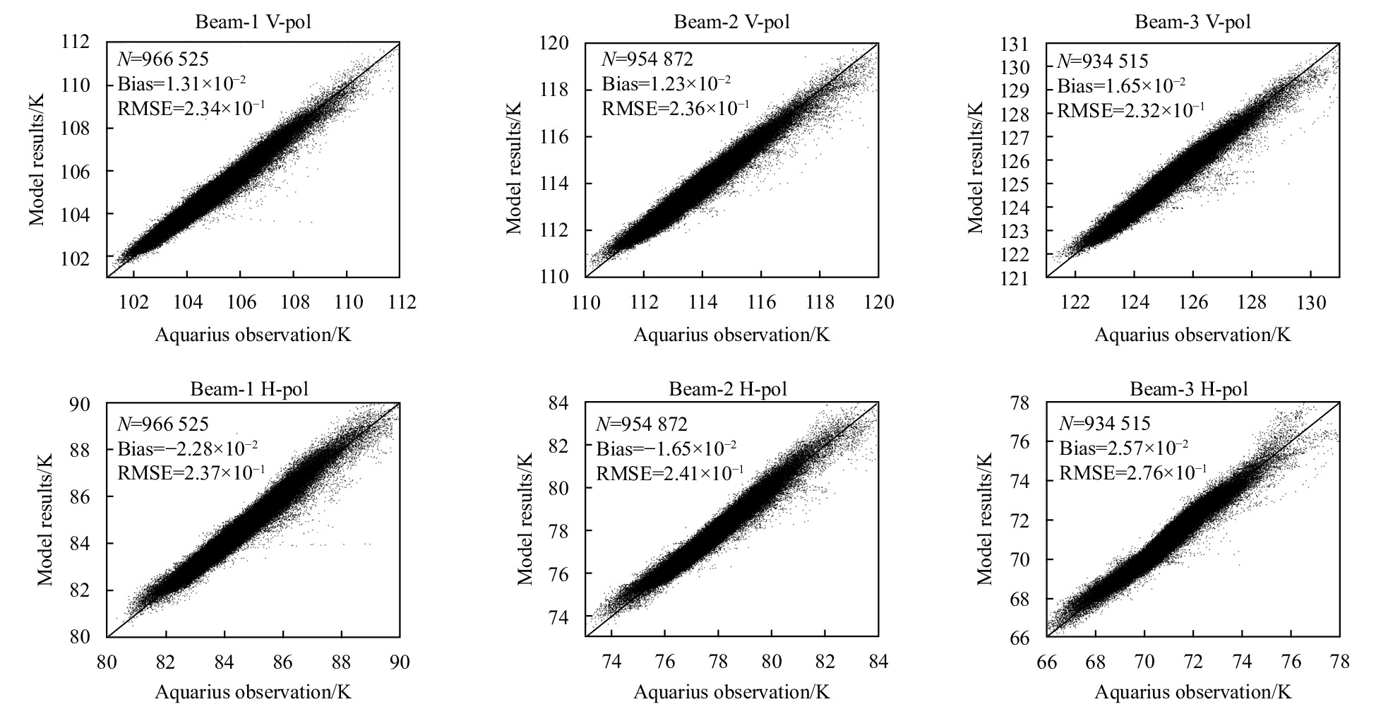
Figure 5 presents the comparison of the total surface TBs calculated using MLE1 and that observed by Aquarius. It can be seen that the number of data points in each band is greater than 900 000. Basically, the TB calculated by the model is in good agreement with the measured TB, and the average bias between the two TBs is better than 0.03 K. The RMSE between the two TBs is better than 0.24 K for most incidence angles and polarizations, and the RMSE is relatively higher only at a large incident angle and horizontal polarization. The V-pol results are better than those of H-pol when the incidence angle is the same. From the distribution of scatter points, although the data points affected by factors such as land and rainfall are excluded, a small number of points still show larger bias.

| $$ {\rm{MLE}}2 = \frac{{{{\left({ew - e{w_{{\rm{NRCS}}\_{\rm{HH}}}}} \right)}^2}}}{{Va{r_{{\rm{NRCS}}\_{\rm{HH}}}}}} + \frac{{{{\left({ew - e{w_{{\rm{NCEP}}}}} \right)}^2}}}{{Va{r_{{\rm{NCEP}}}}}} + \frac{{{{\left({ew - e{w_{{\rm{rad}}}}} \right)}^2}}}{{Va{r_{{\rm{rad}}}}}}, $$ | (5) |
where
Table 2 shows the statistical analysis results between the total surface TB measured by Aquarius and that calculated by different methods after using various wind-speed-related data as input. The two columns on the left are calculated from the model mentioned above and the right two columns are from Aquarius’ ATBD and the wind-speed data obtained by different methods. From the results in the table, no matter which method is used, the more data related to the wind speed is used in the calculation, the better the model result. The bias of TB obtained using the model proposed in this paper is generally better than the bias of the method that recalculates the TB by first retrieving the wind speed. When the HH NRCS and NCEP data are used, the RMSE of the TB calculated by the MLE1 method is better than that obtained by HHwind at each polarization and incidence angle. For the two kinds of TB, the RMSE in vertical polarization is better than that in horizontal polarization. In horizontal polarization, the RMSE increases with increasing incidence angle. When radiometer data are added, the RMSE is significantly reduced. The RMSE of TB calculated including the MLE2 method is better than that calculated by HHHwind at the vertical polarization; however, the RMSE is higher at the horizontal polarization because the retrieval of HHHwind itself uses the TB in the horizontal polarization.
| Beam and polarization | HH+NCEP (MLE1) | HH+NCEP+RAD (MLE2) | V5 model-HHwind | V5 model-HHHwind | |||||||
| Bias/K | RMSE/K | Bias/K | RMSE/K | Bias/K | RMSE/K | Bias/K | RMSE/K | ||||
| Beam-1 V | 1.31×10⁻² | 2.34×10⁻¹ | 2.34×10⁻² | 2.08×10⁻¹ | –3.41×10⁻² | 2.43×10⁻¹ | –7.64×10⁻³ | 2.13×10⁻¹ | |||
| Beam-2 V | 1.23×10⁻² | 2.36×10⁻¹ | 1.36×10⁻² | 2.14×10⁻¹ | –3.27×10⁻² | 2.58×10⁻¹ | –2.39×10⁻² | 2.20×10⁻¹ | |||
| Beam-3 V | 1.65×10⁻² | 2.32×10⁻¹ | 2.01×10⁻² | 2.13×10⁻¹ | –4.15×10⁻² | 2.42×10⁻¹ | –3.04×10⁻² | 2.23×10⁻¹ | |||
| Beam-1 H | –2.28×10⁻² | 2.37×10⁻¹ | –2.85×10⁻² | 2.11×10⁻¹ | –4.31×10⁻² | 2.63×10⁻¹ | –3.45×10⁻² | 2.02×10⁻¹ | |||
| Beam-2 H | –1.65×10⁻² | 2.41×10⁻¹ | –2.51×10⁻² | 2.19×10⁻¹ | –1.60×10⁻² | 2.78×10⁻¹ | –5.25×10⁻² | 2.04×10⁻¹ | |||
| Beam-3 H | 2.57×10⁻³ | 2.76×10⁻¹ | –1.78×10⁻² | 2.47×10⁻¹ | –1.16×10⁻² | 2.79×10⁻¹ | –4.41×10⁻² | 2.10×10⁻¹ | |||
DownLoad:
CSV
In this paper, a new method for wind-induced TB correction by directly using the NRCS measured by a scatterometer aboard the Aquarius/SAC-D satellite is presented that can be used for roughness correction of ocean emissivity without ancillary wind-speed data. Compared with the previous method of using the retrieved wind speed, the new method is more tractable since the intermediate steps of wind-speed retrieval are reduced, so that the calculation accuracy of the TB can be improved.
With more available data for the correction of TB, maximum likelihood estimation is used to include the results of wind-induced emissivity computed from various data. Compared to the Aquarius standard algorithms using retrieved wind speed from various data sources, the proposed method shows better performance in calculation accuracy.
According to the distribution of the RMSE between the wind-induced emissivity calculated from the model and observations in different wind directions, the proposed method based on NRCS measurements has relatively low accuracy for roughness correction in crosswind directions. In future satellite design, high-frequency radiometers or scatterometer observations with a 90° azimuth observation difference may be more suitable for correcting wind-induced roughness.
The Aquarius L2 data were provided by NASA PO.DAAC at the Jet Propulsion Laboratory (
| [1] |
Camps A, Font J, Vall-Llossera M, et al. 2004. The WISE 2000 and 2001 field experiments in support of the SMOS mission: sea surface L-band brightness temperature observations and their application to sea surface salinity retrieval. IEEE Transactions on Geoscience and Remote Sensing, 42(4): 804–823. doi: 10.1109/TGRS.2003.819444
|
| [2] |
Dinnat E P, Boutin J, Caudal G, et al. 2003. On the use of EUROSTARRS and WISE data for validating L-band emissivity models. In: Proceedings of the First Results Workshop on Eurostarrs, Wise, Losac Campaigns. Noordwijk, Netherlands: ESA, 117–124
|
| [3] |
Du Yanlei, Yang Xiaofeng, Chen Kunshan, et al. 2017. An improved spectrum model for sea surface radar backscattering at L-Band. Remote Sensing, 9(8): 776. doi: 10.3390/rs9080776
|
| [4] |
Etcheto J, Dinnat E P, Boutin J, et al. 2004. Wind speed effect on L-band brightness temperature inferred from EuroSTARRS and WISE 2001 field experiments. IEEE Transactions on Geoscience and Remote Sensing, 42(10): 2206–2213. doi: 10.1109/TGRS.2004.834644
|
| [5] |
Fore A G, Yueh S H, Tang Wenqiang, et al. 2014. Aquarius wind speed products: algorithms and validation. IEEE Transactions on Geoscience and Remote Sensing, 52(5): 2920–2927. doi: 10.1109/TGRS.2013.2267616
|
| [6] |
Guimbard S, Gourrion J, Portabella M, et al. 2012. SMOS semi-empirical ocean forward model adjustment. IEEE Transactions on Geoscience and Remote Sensing, 50(5): 1676–1687. doi: 10.1109/TGRS.2012.2188410
|
| [7] |
Hollinger J P. 1971. Passive microwave measurements of sea surface roughness. IEEE Transactions on Geoscience Electronics, 9(3): 165–169. doi: 10.1109/TGE.1971.271489
|
| [8] |
Isoguchi O, Shimada M. 2009. An L-band ocean geophysical model function derived from PALSAR. IEEE Transactions on Geoscience and Remote Sensing, 47(7): 1925–1936. doi: 10.1109/TGRS.2008.2010864
|
| [9] |
Lagerloef G, Colomb F, Le Vine D, et al. 2008. The Aquarius/SAC-D mission: designed to meet the salinity remote-sensing challenge. Oceanography, 21(1): 68–81. doi: 10.5670/oceanog.2008.68
|
| [10] |
Ma Wentao, Yang Xiaofeng, Liu Guihong, et al. 2014. An improved model for L-band brightness temperature estimation over foam-covered seas under low and moderate winds. IEEE Journal of Selected Topics in Applied Earth Observations and Remote Sensing, 7(9): 3784–3793. doi: 10.1109/JSTARS.2014.2318432
|
| [11] |
Meissner T, Wentz F J. 2004. The complex dielectric constant of pure and sea water from microwave satellite observations. IEEE Transactions on Geoscience and Remote Sensing, 42(9): 1836–1849. doi: 10.1109/TGRS.2004.831888
|
| [12] |
Meissner T, Wentz F J. 2012. The emissivity of the ocean surface between 6 and 90 GHz over a large range of wind speeds and earth incidence angles. IEEE Transactions on Geoscience and Remote Sensing, 50(8): 3004–3026. doi: 10.1109/TGRS.2011.2179662
|
| [13] |
Meissner T, Wentz F, Hilburn K, et al. 2012. The aquarius salinity retrieval algorithm. In: Proceedings of 2012 IEEE International Geoscience and Remote Sensing Symposium. Munich, Germany: IEEE, 386–388
|
| [14] |
Meissner T, Wentz F J, Le Vine D M. 2018. The salinity retrieval algorithms for the NASA aquarius version 5 and SMAP version 3 releases. Remote Sensing, 10(7): 1121. doi: 10.3390/rs10071121
|
| [15] |
Meissner T, Wentz F J, Ricciardulli L. 2014. The emission and scattering of L-band microwave radiation from rough ocean surfaces and wind speed measurements from the Aquarius sensor. Journal of Geophysical Research: Oceans, 119(9): 6499–6522. doi: 10.1002/2014JC009837
|
| [16] |
Reul N, Grodsky S A, Arias M, et al. 2020. Sea surface salinity estimates from spaceborne L-band radiometers: an overview of the first decade of observation (2010–2019). Remote Sensing of Environment, 242: 111769. doi: 10.1016/j.rse.2020.111769
|
| [17] |
Yin Xiaobin, Boutin J, Dinnat E, et al. 2016. Roughness and foam signature on SMOS-MIRAS brightness temperatures: a semi-theoretical approach. Remote Sensing of Environment, 180: 221–233. doi: 10.1016/j.rse.2016.02.005
|
| [18] |
Yin Xiaobin, Boutin J, Martin N, et al. 2012. Optimization of L-band sea surface emissivity models deduced from SMOS data. IEEE Transactions on Geoscience and Remote Sensing, 50(5): 1414–1426. doi: 10.1109/TGRS.2012.2184547
|
| [19] |
Yueh S H, Dinardo S J, Fore A G, et al. 2010. Passive and active L-band microwave observations and modeling of ocean surface winds. IEEE Transactions on Geoscience and Remote Sensing, 48(8): 3087–3100. doi: 10.1109/TGRS.2010.2045002
|
| [20] |
Yueh S H, Tang Wenqing, Fore A G, et al. 2013. L-band passive and active microwave geophysical model functions of ocean surface winds and applications to Aquarius retrieval. IEEE Transactions on Geoscience and Remote Sensing, 51(9): 4619–4632. doi: 10.1109/TGRS.2013.2266915
|
| [21] |
Yueh S H, West R, Wilson W J, et al. 2001. Error sources and feasibility for microwave remote sensing of ocean surface salinity. IEEE Transactions on Geoscience and Remote Sensing, 39(5): 1049–1060. doi: 10.1109/36.921423
|
| 1. | Yongqing Liu, Te Wang, Risheng Yun, et al. Analysis of Onboard Verification Flight Test for the Salinity Satellite Scatterometer. Sensors, 2023, 23(21): 8846. doi:10.3390/s23218846 |

Figures(5) / Tables(2)

Supported by:
Beijing Renhe Information Technology Co. Ltd

Wentao Ma, Guihong Liu, Yang Yu, Yanlei Du. Roughness correction method for salinity remote sensing using combined active/passive observations[J]. Acta Oceanologica Sinica, 2021, 40(11): 189-195. doi: 10.1007/s13131-021-1744-z

| Beamand polarization | VV | HH | NCEP | |||||
| Bias/K | RMSE/K | Bias/K | RMSE/K | Bias/K | RMSE/K | |||
| Beam-1 V | –6.81×10⁻³ | 3.31×10⁻¹ | 1.77×10⁻³ | 2.77×10⁻¹ | –4.25×10⁻² | 3.34×10⁻¹ | ||
| Beam–2 V | –1.34×10⁻² | 3.99×10⁻¹ | 3.96×10⁻³ | 2.81×10⁻¹ | –2.95×10⁻² | 3.42×10⁻¹ | ||
| Beam–3 V | –9.60×10⁻³ | 3.73×10⁻¹ | 6.59×10⁻³ | 2.59×10⁻¹ | –3.96×10⁻² | 3.16×10⁻¹ | ||
| Beam–1 H | –1.72×10⁻² | 4.13×10⁻¹ | –4.83×10⁻³ | 3.28×10⁻¹ | –4.67×10⁻² | 3.44×10⁻¹ | ||
| Beam–2 H | –9.90×10⁻³ | 5.61×10⁻¹ | 1.53×10⁻² | 3.57×10⁻¹ | –2.61×10⁻³ | 3.75×10⁻¹ | ||
| Beam–3 H | –1.56×10⁻² | 6.17×10⁻¹ | 1.47×10⁻² | 3.84×10⁻¹ | 1.89×10⁻³ | 3.95×10⁻¹ | ||
DownLoad:
CSV
| Beam and polarization | HH+NCEP (MLE1) | HH+NCEP+RAD (MLE2) | V5 model-HHwind | V5 model-HHHwind | |||||||
| Bias/K | RMSE/K | Bias/K | RMSE/K | Bias/K | RMSE/K | Bias/K | RMSE/K | ||||
| Beam-1 V | 1.31×10⁻² | 2.34×10⁻¹ | 2.34×10⁻² | 2.08×10⁻¹ | –3.41×10⁻² | 2.43×10⁻¹ | –7.64×10⁻³ | 2.13×10⁻¹ | |||
| Beam-2 V | 1.23×10⁻² | 2.36×10⁻¹ | 1.36×10⁻² | 2.14×10⁻¹ | –3.27×10⁻² | 2.58×10⁻¹ | –2.39×10⁻² | 2.20×10⁻¹ | |||
| Beam-3 V | 1.65×10⁻² | 2.32×10⁻¹ | 2.01×10⁻² | 2.13×10⁻¹ | –4.15×10⁻² | 2.42×10⁻¹ | –3.04×10⁻² | 2.23×10⁻¹ | |||
| Beam-1 H | –2.28×10⁻² | 2.37×10⁻¹ | –2.85×10⁻² | 2.11×10⁻¹ | –4.31×10⁻² | 2.63×10⁻¹ | –3.45×10⁻² | 2.02×10⁻¹ | |||
| Beam-2 H | –1.65×10⁻² | 2.41×10⁻¹ | –2.51×10⁻² | 2.19×10⁻¹ | –1.60×10⁻² | 2.78×10⁻¹ | –5.25×10⁻² | 2.04×10⁻¹ | |||
| Beam-3 H | 2.57×10⁻³ | 2.76×10⁻¹ | –1.78×10⁻² | 2.47×10⁻¹ | –1.16×10⁻² | 2.79×10⁻¹ | –4.41×10⁻² | 2.10×10⁻¹ | |||
DownLoad:
CSV
| Beamand polarization | VV | HH | NCEP | |||||
| Bias/K | RMSE/K | Bias/K | RMSE/K | Bias/K | RMSE/K | |||
| Beam-1 V | –6.81×10⁻³ | 3.31×10⁻¹ | 1.77×10⁻³ | 2.77×10⁻¹ | –4.25×10⁻² | 3.34×10⁻¹ | ||
| Beam–2 V | –1.34×10⁻² | 3.99×10⁻¹ | 3.96×10⁻³ | 2.81×10⁻¹ | –2.95×10⁻² | 3.42×10⁻¹ | ||
| Beam–3 V | –9.60×10⁻³ | 3.73×10⁻¹ | 6.59×10⁻³ | 2.59×10⁻¹ | –3.96×10⁻² | 3.16×10⁻¹ | ||
| Beam–1 H | –1.72×10⁻² | 4.13×10⁻¹ | –4.83×10⁻³ | 3.28×10⁻¹ | –4.67×10⁻² | 3.44×10⁻¹ | ||
| Beam–2 H | –9.90×10⁻³ | 5.61×10⁻¹ | 1.53×10⁻² | 3.57×10⁻¹ | –2.61×10⁻³ | 3.75×10⁻¹ | ||
| Beam–3 H | –1.56×10⁻² | 6.17×10⁻¹ | 1.47×10⁻² | 3.84×10⁻¹ | 1.89×10⁻³ | 3.95×10⁻¹ | ||
| Beam and polarization | HH+NCEP (MLE1) | HH+NCEP+RAD (MLE2) | V5 model-HHwind | V5 model-HHHwind | |||||||
| Bias/K | RMSE/K | Bias/K | RMSE/K | Bias/K | RMSE/K | Bias/K | RMSE/K | ||||
| Beam-1 V | 1.31×10⁻² | 2.34×10⁻¹ | 2.34×10⁻² | 2.08×10⁻¹ | –3.41×10⁻² | 2.43×10⁻¹ | –7.64×10⁻³ | 2.13×10⁻¹ | |||
| Beam-2 V | 1.23×10⁻² | 2.36×10⁻¹ | 1.36×10⁻² | 2.14×10⁻¹ | –3.27×10⁻² | 2.58×10⁻¹ | –2.39×10⁻² | 2.20×10⁻¹ | |||
| Beam-3 V | 1.65×10⁻² | 2.32×10⁻¹ | 2.01×10⁻² | 2.13×10⁻¹ | –4.15×10⁻² | 2.42×10⁻¹ | –3.04×10⁻² | 2.23×10⁻¹ | |||
| Beam-1 H | –2.28×10⁻² | 2.37×10⁻¹ | –2.85×10⁻² | 2.11×10⁻¹ | –4.31×10⁻² | 2.63×10⁻¹ | –3.45×10⁻² | 2.02×10⁻¹ | |||
| Beam-2 H | –1.65×10⁻² | 2.41×10⁻¹ | –2.51×10⁻² | 2.19×10⁻¹ | –1.60×10⁻² | 2.78×10⁻¹ | –5.25×10⁻² | 2.04×10⁻¹ | |||
| Beam-3 H | 2.57×10⁻³ | 2.76×10⁻¹ | –1.78×10⁻² | 2.47×10⁻¹ | –1.16×10⁻² | 2.79×10⁻¹ | –4.41×10⁻² | 2.10×10⁻¹ | |||
 DownLoad:


 DownLoad: