First Institute of Oceanography, Ministry of Natural Resources, Qingdao 266061, China
2.
Laboratory for Regional Oceanography and Numerical Modeling, Pilot National Laboratory for Marine Science and Technology (Qingdao), Qingdao 266237, China
3.
Key Laboratory of Marine Science and Numerical Modeling, Ministry of Natural Resources, Qingdao 266061, China
4.
Department of Atmospheric and Environmental Sciences, University at Albany, State University of New York, Albany, NY 12222, USA
5.
College of Ocean and Meteorology, Guangdong Ocean University, Zhanjiang 524088, China
6.
National Marine Environmental Forecasting Center, Beijing 100081, China
Funds:
The National Key Research and Development Program of China under contract Nos 2018YFC1407205 and 2018YFA0605901; the Basic Scientific Fund for National Public Research Institute of China (ShuXingbei Young Talent Program) under contract No. 2019S06; the National Natural Science Foundation of China under contract Nos 41821004, 42022042 and 41941012; the China-Korea Cooperation Project on Northwestern Pacific Climate Change and its Prediction.
To improve the Arctic sea ice forecast skill of the First Institute of Oceanography-Earth System Model (FIO-ESM) climate forecast system, satellite-derived sea ice concentration and sea ice thickness from the Pan-Arctic Ice-Ocean Modeling and Assimilation System (PIOMAS) are assimilated into this system, using the method of localized error subspace transform ensemble Kalman filter (LESTKF). Five-year (2014–2018) Arctic sea ice assimilation experiments and a 2-month near-real-time forecast in August 2018 were conducted to study the roles of ice data assimilation. Assimilation experiment results show that ice concentration assimilation can help to get better modeled ice concentration and ice extent. All the biases of ice concentration, ice cover, ice volume, and ice thickness can be reduced dramatically through ice concentration and thickness assimilation. The near-real-time forecast results indicate that ice data assimilation can improve the forecast skill significantly in the FIO-ESM climate forecast system. The forecasted Arctic integrated ice edge error is reduced by around 1/3 by sea ice data assimilation. Compared with the six near-real-time Arctic sea ice forecast results from the subseasonal-to-seasonal (S2S) Prediction Project, FIO-ESM climate forecast system with LESTKF ice data assimilation has relatively high Arctic sea ice forecast skill in 2018 summer sea ice forecast. Since sea ice thickness in the PIOMAS is updated in time, it is a good choice for data assimilation to improve sea ice prediction skills in the near-real-time Arctic sea ice seasonal prediction.
Observations show that Arctic sea ice has been undergoing significant changes over the past several decades. Arctic sea ice cover derived from passive microwave instruments has shown negative trends in all months since 1979, with the largest decrease in September (Parkinson and Cavalieri, 2008; Parkinson, 2019). The sea ice extent in September has decreased by 3.24×10⁶ km2 during 1979–2017 (Liu et al., 2019). As the Arctic sea ice declines, the sea ice age has decreased continually (Fowler et al., 2004; Nghiem et al., 2007; Maslanik et al., 2011). Based on the estimation of Maslanik et al. (2011), the fraction of multiyear sea ice in March decreased from about 75% in the mid 1980s to 45% in 2011. The thickness of Arctic sea ice has also declined significantly (Kwok and Rothrock, 2009; Laxon et al., 2013; Lindsay and Schweiger, 2015; Kwok and Cunningham, 2015). Over the past 40 years, observed Arctic sea ice thickness in the data available area has decreased by 1.6 m or about 53% (Kwok and Rothrock, 2009). Meanwhile, observations indicate that Arctic sea ice drift has shown gradual acceleration in both winter and summer since 1950s (Hakkinen et al., 2008; Olason and Notz, 2014).
Coupled sea ice-ocean models and fully coupled climate models have been used in Arctic sea ice forecast and prediction. However, based on the seasonal sea ice outlook under Sea Ice Prediction Network (SIPN, https://www.arcus.org/sipn) (Stroeve et al., 2014), the sea ice predictions by dynamical models (both coupled sea ice-ocean models and fully coupled climate models) still deviate from the observations substantially for most years since 2008 (Liu et al., 2019). For the subseasonal-to-seasonal (S2S) Arctic sea ice prediction, Zampieri et al. (2018) shows that there are large differences in predictive skill between different operational forecast systems, with some showing a lack of predictive skill even at short weather time scales and the best producing skilful forecasts more than 1.5 months ahead. To improve Arctic sea ice predictive skill, both the model and the initialization should be improved.
Sea ice data assimilation to generate realistic and skilful model initialization is essential to improve the Arctic sea ice predictive skill, but at present sea ice data assimilation remains a relatively new research area (Liu et al., 2019). Several methods have been used to sea ice parameters assimilation, such as nudging (Tietsche et al., 2013), optimal interpolation (Zhang et al., 2003), variational methods (Hebert et al., 2015; Lemieux et al., 2016), and ensemble Kalman filters (Sakov et al., 2012; Lisæter et al., 2003; Yang et al., 2014, 2015; Chen et al., 2017). The method of ensemble Kalman filters is relatively easy to implement, and is effective for sea ice simulations and forecasts, so it has recently become more common (Liu et al., 2019).
Several sea ice parameters derived from satellite remote sensing, such as sea ice concentration, sea ice thickness, and sea ice drift are available now to be potentially assimilated into the large scale dynamical sea ice models (Liu et al., 2019). Sea ice concentration and thickness are the most commonly used in the Arctic sea ice data assimilation. With sea ice concentration data assimilation, the model simulation capacity and predictive skill of sea ice cover and sea ice extent can be improved by both coupled sea ice-ocean models (Lisæter et al., 2003; Lindsay and Zhang, 2006; Wang et al., 2013b; Yang et al., 2015, 2016; Toyoda et al., 2016) and fully coupled climate models (Tietsche et al., 2013; Wang et al., 2013a; Kimmritz et al., 2018). As the satellite-derived basin-scale Arctic sea ice thickness are produced, sea ice thickness are beginning to be assimilated into the coupled sea ice-ocean models to improve the sea ice thickness simulations and seasonal sea ice forecasts (Lisæter et al., 2017; Lindsay et al., 2012; Yang et al., 2014; Xie et al., 2016; Allard et al., 2018; Mu et al., 2018). The studies of Chevallier and Salas-Mélia (2012) and Day et al. (2014) indicate that accurate knowledge of Arctic sea ice thickness field is crucial for sea ice prediction at longer time scales. Based on the National Centers for Environmental Prediction (NCEP) climate forecast system, reanalysis and satellite-derived sea ice thickness have been assimilated by Collow et al. (2015) and Chen et al. (2017), respectively, and the systematic bias in the predicted ice thickness is dramatically reduced. Blockley and Peterson (2018) assimilated winter CryoSat-2 sea ice thickness into the Met Office’s coupled seasonal prediction system, and they found the skill of summer seasonal predictions is significantly improved.
The purposes of this paper are to study Arctic sea ice concentration and thickness assimilation in First Institute of Oceanography-Earth System Model (FIO-ESM) climate forecast system, and to assess the predictive skill in a near-real-time Arctic sea ice forecast in August 2018.
2.
Model and data
2.1
Model
This study is based on FIO-ESM climate forecast system. The model used in this system is FIO-ESM v1.0, which is developed by Qiao et al. (2013). It is the first fully coupled earth system model including the surface wave model through including the non-breaking wave-induced vertical mixing (Qiao et al., 2004) into the ocean circulation model. The physical model components are the Community Atmosphere Model Version 3 (CAM3) (Collins et al., 2006), the Community Land Model Version 3.5 (CLM3.5) (Dickinson et al., 2006), the Los Alamos National Laboratory sea ice model Version 4 (CICE4) (Hunke and Lipscomb, 2008), the Parallel Ocean Program Version 2.0 (POP2.0) (Smith et al., 2010), and the MASNUM surface wave model (Yang et al., 2005). The horizontal resolution of the CAM3 is T42 spectral truncation (about 2.875°), nominal 1° for POP2.0 and CICE4. The number of vertical layer in the atmosphere and ocean models is 26 and 40, respectively. Five ice thickness categories with the lower bounds of 0 m, 0.64 m, 1.39 m, 2.47 m, and 4.57 m are used in FIO-ESM. The detail of FIO-ESM can be found in Qiao et al. (2013).
2.2
Data
For ocean data assimilation, satellite observed daily sea surface temperature (SST) and sea level anomaly (SLA) were used. SST was from satellites of Advanced Very High Resolution Radiometer (NOAA-AVHRR) and Advanced Microwave Scanning Radiometer-Earth Observing System (AMSR-E), with a horizontal resolution of (1/4)°×(1/4)° (Reynolds et al., 2007), provided by the Climate Data Center of National Oceanic and Atmospheric Administration (NOAA). SLA was from Archiving, Validation and Interpretation of Satellite Data in Oceanography (AVISO) (Ducet et al., 2000), with a horizontal resolution of (1/3)°×(1/3)°. During data assimilation, SST and SLA were assimilated only in the open water regions. For ice-covered regions, ocean state is not adjusted directly by the assimilation.
For sea ice data assimilation, two satellite-derived sea ice concentration products from EUMETSAT OSI SAF (http://osisaf.met.no) and modelled sea ice thickness from the the Pan-Arctic Ice-Ocean Modeling and Assimilation System (PIOMAS) reanalysis (http://psc.apl.uw.edu/research/projects/arctic-sea-ice-volume-anomaly/data/model_grid) were used. The first sea ice concentration product is OSI-409/-a, which is derived using passive microwave data from the SMMR, SSM/I and SSMIS sensors before 15 April 2015, and using SSMIS sensors after 16 April 2015. The deviations between this ice product and the ice charts are large during summer melt (up to −20%), while during the winter the negative deviations are 5%–10%. So 15% was used to represent observational error during data assimilation in this study. The second product used is OSI-408, which is computed from atmospherically corrected AMSR-2 brightness temperatures. Its total standard deviation is about 13% comparison with ice charts. So the observational error of 15% was used to kept the same as the first product. During assimilation experiment, OSI-409/-a was used during 2014 to 2017, and OSI-408 was used in 2018. The spatial resolutions of these two sea ice concentration products are both 10 km. Daily Arctic sea ice thickness used in data assimilation was from PIOMAS, provided by the Polar Science Center at the University of Washington. PIOMAS is a numerical model with components for sea ice and ocean and the capacity for assimilating sea ice concentration and SST (Zhang and Rothrock, 2003). PIOMAS sea ice thickness estimates agree well with in situ observation, airborne and satellite measurements (Zhang and Rothrock, 2003; Schweiger et al., 2011; Laxon et al., 2013). It has been widely used in the Arctic climate studies. Collow et al. (2015) reported that Arctic sea ice prediction can be improved using PIOMAS initial sea ice thickness in the NCEP climate forecast system. Compared with observations, the root mean square error of PIOMAS sea ice thickness is 0.61 m in spring, and 0.76 m in autumn (Schweiger et al., 2011). So here the mean value of 0.685 m was used as the data uncertainty during assimilation.
For assimilation result assessment, several independent datasets were used in this study. Satellite-derived sea ice extent from the National Snow and Ice Data Centre (NSIDC) (ftp://sidads.colorado.edu/DATASETS/NOAA/G02135/; Fetterer et al., 2017) was used to assess the simulated sea ice extent. During sea ice concentration assessment, daily sea ice concentration derived based on the National Aeronautics and Space Administration (NASA) team algorithm (Cavalieri et al., 1996) provided by the NSIDC (http://nsidc.org/data/seaice/) was selected. Observed sea ice thickness from the Operation IceBridge (https://nsidc.org/data/NSIDC-0708/versions/1) and winter season (October–April) weekly sea ice thickness product based on the CryoSat-2 and SMOS merged data (Ricker et al., 2017) (http://data.seaiceportal.de/gallery/index_new.php) was used to evaluate the modeled sea ice thickness. In order to intercompare near-real-time sea ice forecasts, six forecast results from S2S Prediction Project (http://www.s2sprediction.net/) were also used. These six S2S sea ice forecasts were provided by CMA, ECMWF, KMA, Meteo France, NCEP and UKMO, which have dynamical sea ice models in their forecast systems.
3.
Assimilation method and experiment design
3.1
Assimilation method
The ocean data assimilation method applied in the FIO-ESM climate forecast system is Ensemble Adjustment Kalman Filter (EAKF), which assimilates satellite observed SST and SLA (Yin, 2015; Chen et al., 2016). There is no in-situ temperature and salinity profiles assimilated. With EAKF ocean satellite data assimilation, FIO-ESM modeled ocean temperature and salinity biases are reduced significantly (Yin, 2015; Chen et al., 2016), and the long-term trend of Arctic sea ice extent in this system is also dramatically improved compared with free run result (Shu et al., 2015).
Sea ice data assimilation method used here follows Chen et al. (2017), but with some differences. The method is the ensemble-based localized error subspace transform ensemble Kalman filter (LESTKF) implemented in the parallel data assimilation framework (PDAF) (Nerger and Hiller, 2013). After reviewing different kinds of assimilation method, Liu et al. (2019) recommends the LESTKF for sea ice data assimilation. Chen et al. (2017) shows that systemic bias of modeled sea ice concentration and thickness can be reduced dramatically by performing sea ice assimilation every 5 days using the LESTKF. Different from Chen et al. (2017), sea ice data was assimilated every day in this study.
The LESTKF consists of four steps: initialization, forecast, analysis, and ensemble transformation. For the initialization step, the method recommended by PDAF is that initial ensembles are generated from the leading modes of the modeled sea ice state vectors, which provide an estimate of initial model states and uncertainties prior to the evolution of forecasts. This method was used in Chen et al. (2017). But in this study, 10 ensembles in the FIO-ESM climate forecast system were used directly; since the 10 ensembles have been generated already during ocean data assimilation by a tiny-perturbing method through three-dimensional ocean temperature perturbed the FIO-ESM climate forecast system (Chen et al., 2016). For the tiny-perturbing method, only the ocean temperature in three dimensions was perturbed, which can be expressed by the following formula:
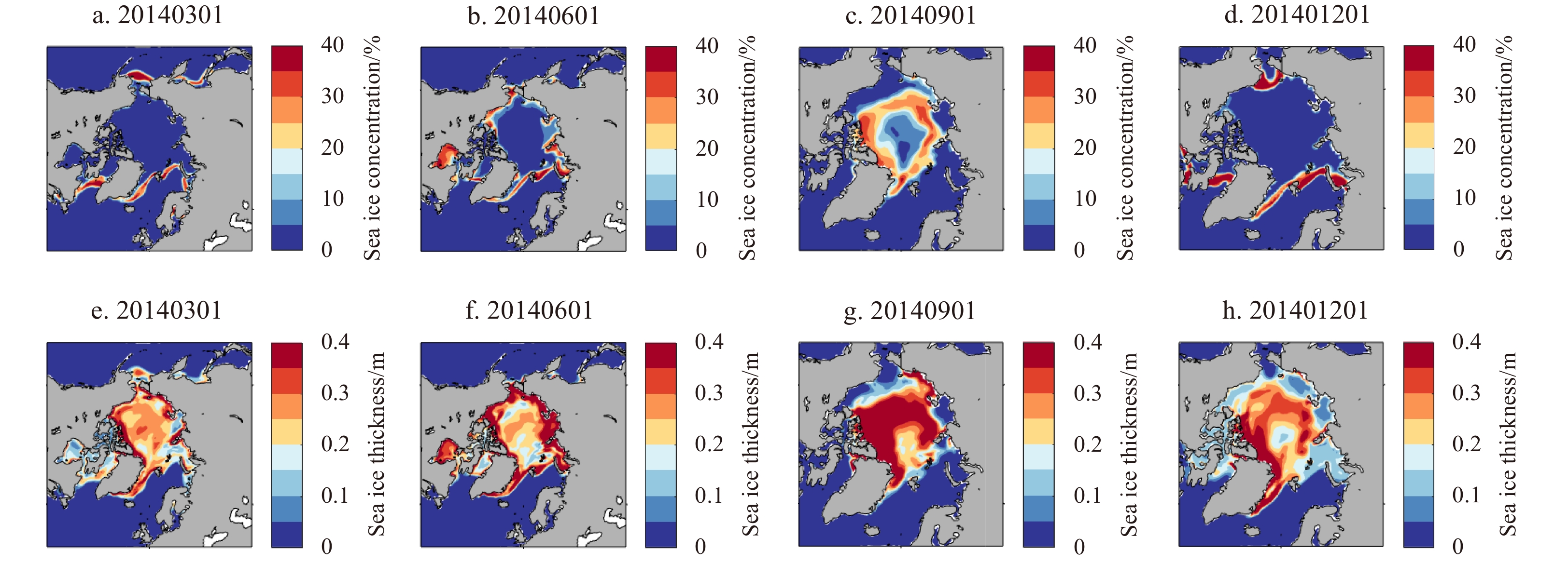
where $ \alpha $ is a small value equal to 10−3, and $ \beta $ is a random number within the range of (−1, 1). For different ensembles, different random seeds are used to generate the random number at each model grid. The subscripts i, j and k are the indices of the model grid, and the superscripts “pert” and “init” represent the state before and after perturbation, respectively. The dynamic relationship of variables in the model can be well maintained and the imbalance due to the perturbation on the initial conditions significantly reduced using this tiny-perturbing method. The sea ice concentration and thickness spreads for these 10 ensembles in 2014 were checked (Fig. 1). Sea ice concentration spread is large in the marginal ice zone and small in the ice covered regions, which shares the similar feature of the uncertainty of satellite observed sea ice concentration. Sea ice thickness spread is mainly <0.4 m in most regions in winter season, but can exceed 0.4 m in September. So these 10 ensembles can be used for sea ice data assimilation. For the second step, all the 10 ensembles were dynamically evolved with the FIO-ESM climate forecast system. For the third step, the LESTKF was used to assimilate satellite-derived sea ice concentration and PIOMAS thickness, considering the observational errors and background uncertainty represented by the spread of model realizations. In the regulated localization scheme, an influential cutoff distance of four model grid points (about 160 km in the Arctic Ocean) was used. For the last step, all the 10 ensembles were transformed to new states while preserving the ensemble mean and covariance.
Figure
1.
Ensemble spread (one standard deviation) of simulated sea ice concentration (a–d) and sea ice thickness (e–h) on the first day of March (a, e), June (b, f), September (c, g), and December (d, h) 2014 in the FIO-ESM climate forecast system.
FIO-ESM forecast system uses five ice categories to describe the evolution of sea ice thickness distribution. However, satellite-derived ice concentration and PIOMAS ice thickness only provide the aggregated values. So a scheme is required to remap the updated aggregated sea ice parameters to model ice categories after the data assimilation (Liu et al., 2019). Another difference with Chen et al. (2017) is the remap scheme. In Chen et al. (2017), the analysis is remapped to the categories keeping the ratios of the ice concentration (volume) in each category the same as the value before data assimilation, and then ice thickness is shifted to the adjacent category to meet the thickness limitation. In this study, the increment of ice concentration, thickness and energy are first added (subtracted) only to (from) the thinnest category, and then ice area, thickness and energy are shifted to the adjacent category to meet the thickness limitation. For the snow on sea ice, its mass is kept during data assimilation. But if there is no sea ice, snow mass is set to zero.
3.2
Experiment design
With the development of the FIO-ESM climate forecast system, it can not only be used as a new tool to study the impacts of assimilating sea ice data in coupled model simulations, but also be used for realistic sea ice forecast. In this paper the potential applications of the system using two sets of experiments are demonstrated.
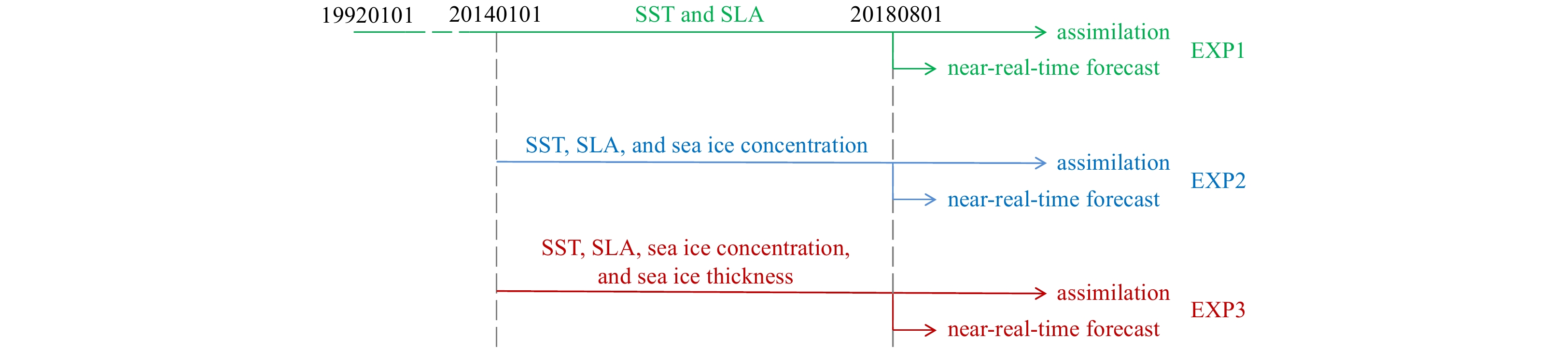
In the first set of experiments three numerical experiments (EXP1, EXP2, and EXP3) which assimilate different observational data are carried out to assess the impacts of assimilating sea ice data. In EXP1, satellite-observed SST and SLA from first January 1992 to the end of 2018 are assimilated. This experiment is the extension of the standard assimilation experiment described by Song et al. (2015). EXP2 and EXP3 branched out from the results of EXP1 on 1 January 2014 and were run until the end of 2018. In EXP2, satellite-observed sea ice concentration and SST and SLA as well are assimilated. In EXP3, the sea ice thickness provided by PIOMAS is also assimilated besides the data assimilated in EXP2. The data assimilated in the three experiments are summarized in Table 1. By comparing EXP1 and EXP2, the impact of assimilating sea ice concentration can be studied; by comparing EXP2 and EXP3, the impact of assimilating sea ice thickness can be investigated. The overall effect of assimilating sea ice concentration and thickness can be revealed by comparing EXP1 and EXP3.
In the second set of experiments near-real-time two-month forecast with three experiments are carried out. They were initialized using the results on 1 August 2018 obtained from the three assimilation experiments described above, respectively. During the forecast simulations, data assimilation was switched off to learn how the initial condition can influence the forecast. Figure 2 illustrates the configuration and timeline of all the experiments.
For first set of experiments, 5-year (2014–2018) results from EXP1, EXP2, and EXP3 were compared with the observations. For the second set of experiments, two-month (August and September of 2018) near-real-time forecast results from EXP1, EXP2, and EXP3 were compared with S2S Prediction Project results and the observations. The sea ice concentration and extent observations used for result assessment are from OSI SAF, which were introduced in Section 2.
4.
Results
4.1
Sea ice extent and concentration assessment
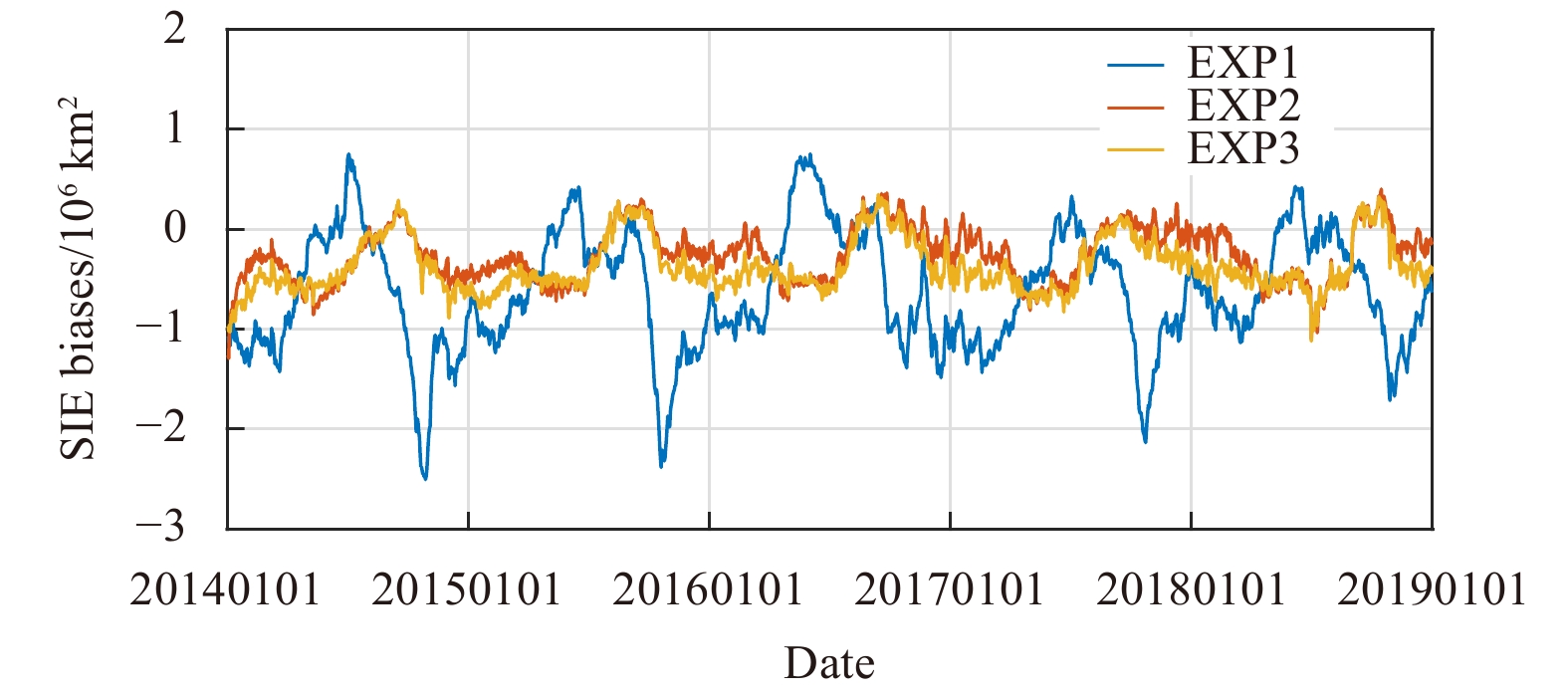
Figure 3 is the comparison of 5-year time-series of Arctic sea ice extent biases from EXP1, EXP2 and EXP3 with satellite-derived sea ice extent from NSIDC, which is derived using different algorithm. Here modeled sea ice extent is calculated as the sum of the area of each grid cell with ice concentration greater than 15%, which is same as the algorithm of satellite-derived sea ice extent. Figure 3 shows that sea ice data assimilation in the FIO-ESM climate forecast system can reduce the sea ice extent bias effectively. SIE root-mean-square error (RMSE) in EXP1 is 0.91×10⁶ km2. With sea ice concentration assimilation, SIE RMSE in EXP2 is only 0.36×10⁶ km2, so about 60% model bias can be reduced. SIE RMSE in EXP3 is 0.45×10⁶ km2. Although the error of EXP3 is a little larger than that in EXP2, about 50% model bias has been reduced compared with EXP1. In fact, the SIE difference between EXP2 and EXP3 is comparable to the uncertainties of different satellite-derived SIE datasets.
Figure
3.
Arctic sea ice extent (SIE) biases during 2014 to 2018. Blue, red and yellow lines are from EXP1, EXP2 and EXP3, respectively. The biases are the results between simulations and observations from NSIDC.
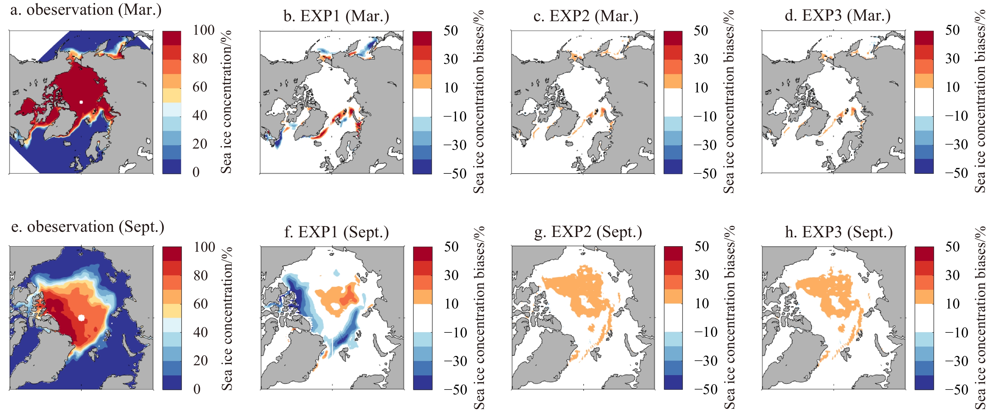
The main problem in EXP1 is that the modeled sea ice cover is less than satellite observations in summer, autumn and winter seasons (Fig. 3). EXP1 modeled winter sea ice cover is insufficient mainly in the marginal ice zone, such as the Bering Sea, Sea of Okhotsk, Labrador Sea, and Gulf of St. Lawrence (Fig. 4). In summer, underestimated sea ice cover is mainly in the Beaufort Sea and Canadian Archipelago (Fig. 4). With sea ice concentration assimilation, most of these problems disappear in EXP2 and EXP3.
Figure
4.
Arctic sea ice concentration observations from NSIDC (a, e) and model biases (b–d and f–h) in March (a–d) and September (e–h) during 2014 to 2018.
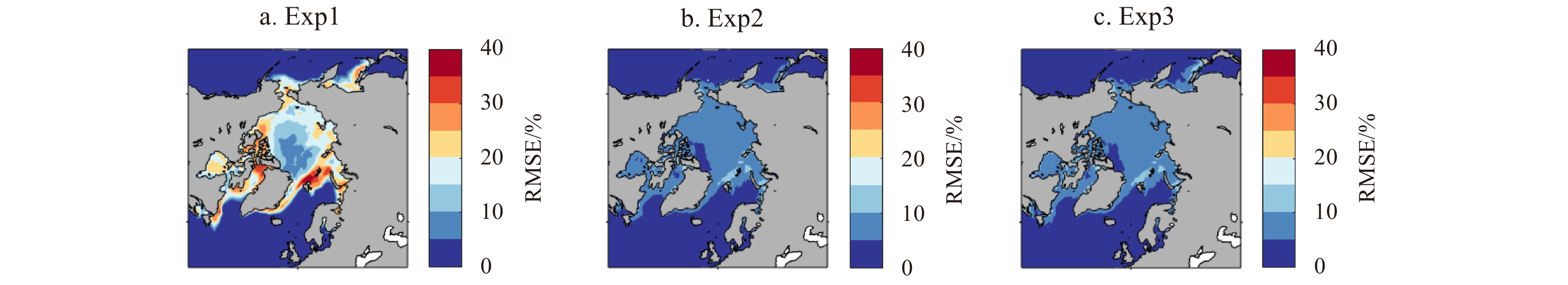
The RMSE of sea ice concentration in Fig. 5 shows that the bias of sea ice concentration can be reduced dramatically by sea ice data assimilation. In EXP1, RMSE in most of the Arctic Ocean is larger than 20%, but it is reduced to less than 10% in EXP2 and EXP3. RMSE in EXP2 and EXP3 has no obvious differences, except in the Sea of Okhotsk, where EXP3 has larger bias than EXP2. This is the main reason why SIE RMSE (0.45×10⁶ km2) in EXP3 is larger than that (0.36×10⁶ km2) in EXP2. It is maybe caused by the setup in sea ice thickness assimilation. In EXP3, for any grid point, if the observed ice concentration is positive but the PIOMAS ice thickness is 0 m, then the ice concentration is set to 0 during data assimilation. An alternative method may help to further reduce the bias in EXP3, such as the scheme used in Tietsche et al. (2013) and Chen et al. (2017). In that scheme, if the observed ice concentration is positive but the ice thickness is 0 m, then the ice thickness is set to 2 m multiplied by the ice concentration.
Figure
5.
Root mean square error (RMSE) of Arctic sea ice concentration during 2014 to 2018. a, b, and c are from EXP1, EXP2, and EXP3, respectively.
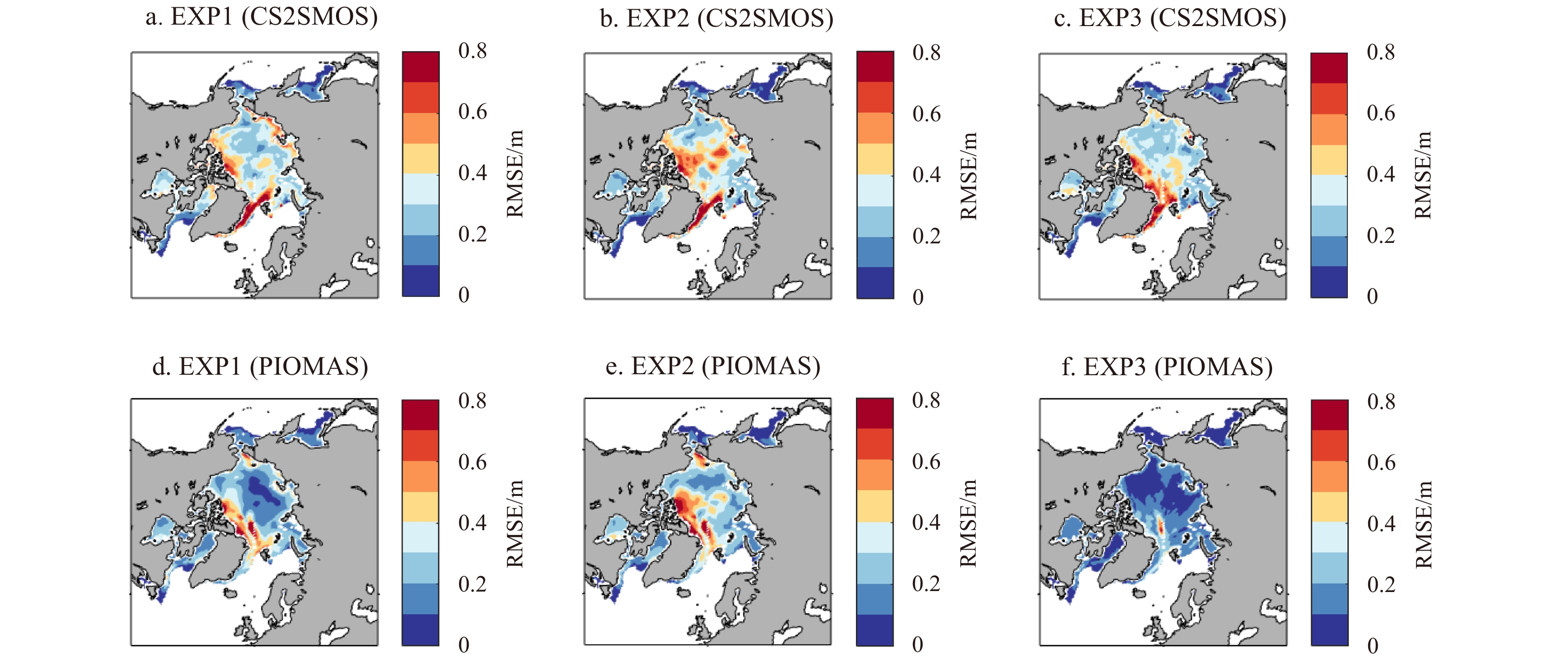
A 5-year time-series of Arctic sea ice volume is compared with PIOMAS in Fig. 6. All the EXP1, EXP2 and EXP3 modeled sea ice volume is less than PIOMAS. Statistical results indicate that the sea ice volume RMSE in EXP1, EXP2, and EXP3 is 2.3×10³ km3, 2.9×10³ km3, and 1.9×10³ km3 respectively. EXP3 has the smallest sea ice volume bias. In EXP2, sea ice volume has some improvement in summer, but has larger bias in winter compared with EXP1. This means that sea ice concentration assimilation has no significant improvement of sea ice thickness in this climate forecast system. The RMSE of sea ice thickness compared to the CryoSat-2 and SMOS merged ice thickness product and PIOMAS ice thickness for the five winter seasons were calculated (Fig. 7). The large ice thickness bias is mainly in the thick ice regions. Compared with the independent CryoSat-2 and SMOS merged ice thickness, EXP1, EXP2, and EXP3 have similar RMSE, with RMSE value averaged in the Arctic Ocean of 0.28 m, 0.25 m, and 0.24 m, respectively. But compared with the PIOMAS ice thickness, the ice thickness bias in EXP3 is reduced significantly. The EXP3 RMSE is less than 0.2 m in most Arctic Ocean. The Arctic Ocean mean RMSE in EXP1, EXP2, and EXP3 is 0.20 m, 0.21 m, and 0.11 m, respectively. The probability density function (PDF) distribution of ice thickness bias compared with IceBridge observations in Fig. 8 shows that simulated sea ice thickness has negative system errors. The ice thickness biases in EXP1, EXP2, and EXP3 compared with IceBridge observations are −0.73 m, −0.62 m, and −0.35 m, respectively. EXP3 has the smallest error.
Figure
6.
Arctic sea ice volume (SIV) during 2014 to 2018 in the PIOMAS, EXP1, EXP2, and EXP3.
Figure
7.
Root mean square error (RMSE) of winter season Arctic sea ice thickness during 2014 to 2018. a–c are calculated based on the CryoSat-2 and SMOS (CS2SMOS) merged sea ice thickness. d–f are calculated based on PIOMAS sea ice thickness.
Figure
8.
Location of IceBridge observations during 2014–2018 (a) and the probability density function (PDF) distribution of modeled sea ice thickness biases compared with IceBridge observations in EXP1, EXP2, and EXP3 (b). The legend in a is the time of the observations.
The realistic spatial distribution of ice thickness can help to improve sea ice predictions for longer time scale. So the spatial correlation coefficients between modeled ice thickness and PIOMAS ice thickness were assessed (Fig. 9). In EXP1, the correlation is high in winter seasons, but decreases quickly during melting seasons, and has the minimum in summer. The EXP2 correlation coefficient is larger than that in EXP1, but it is also restively small in summer reasons. Correlation coefficient in EXP3 increases quickly at beginning of the data assimilation and then keeps quite steady with large correlation coefficient and no drop during melting seasons. The mean correlation coefficient in EXP1, EXP2, and EXP3 is 0.73, 0.76, and 0.95, respectively. Therefore, the spatial correlation between modeled ice thickness and PIOMAS ice thickness is improved significantly through ice thickness assimilation.
Figure
9.
Time series of spatial correlation coefficients between PIOMAS and modeled Arctic sea ice thickness during 2014 to 2018. Blue, red and yellow lines are for EXP1, EXP2 and EXP3, respectively.
The assimilation results indicate that ice concentration assimilation can result in better modeled ice concentration and extent, but there is no much improvement in ice volume and thickness simulations. However, all the biases of modeled ice concentration, ice cover, ice volume, and ice thickness can be reduced in EXP3 with both ice concentration and thickness assimilated.
4.3
Near-real-time sea ice forecast assessment
The ninth Chinese National Arctic Research Expedition was conducted in the summer 2018. At the beginning of August 2018, the FIO-ESM climate forecast system did a near-real-time Arctic sea ice forecast to provide the following two-month ice condition for this expedition. The forecasting initializations were the August 1 restart files in the three assimilation experiments. Forecast length is two months. The forecast results based on EXP3 initialization were further corrected and then provided for this expedition. In this section, the forecast results (without further correction) were assessed by comparison with six S2S near-real-time Arctic ice forecasts, which have dynamical sea ice model in the S2S Prediction Project. These six S2S ice forecasts are from the China Meteorological Administration (CMA), European Centre for Medium-Range Weather Forecasts (ECMWF), Korea Meteorological Administration (KMA), Météo France, National Centers for Environmental Prediction (NCEP), and UK Met Office (UKMO), respectively.
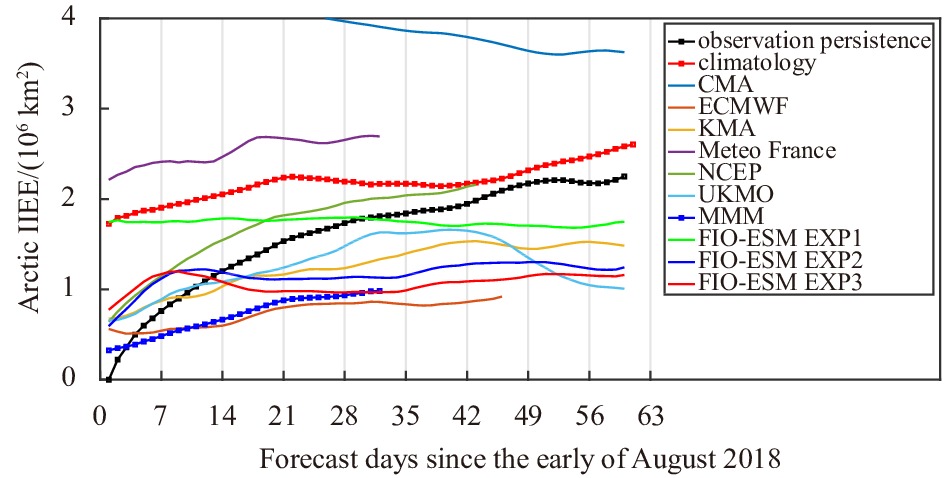
Here the Arctic integrated ice edge error (IIEE) was used during assessment. It is defined as the area where the forecast and the observation disagree on the ice concentration being above or below 15% (Goessling et al., 2016). IIEE is an effective metric to evaluate the forecast skill of ice edge forecast (Goessling et al., 2016; Zampieri et al., 2018). Figure 10 is IIEEs for the six S2S Prediction Project models, FIO-ESM, observation persistence, and climatology forecasts. The IIEE of observation persistence forecast is used as the benchmark to measure the ice forecast skills. Observation persistence forecast is let the observations at the beginning of forecast (1 August 2018 in this case) to be the forecast results. If the IIEE is lower than that of benchmark, the dynamical forecasting system has some predictive skill (Zampieri et al., 2018). Climatology-based benchmark is also used here, which is calculated based on the climatological observations during 1989–2018. The observations are from the same datasets used in data assimilation. Considering the differences in land-sea masks and resolutions of these forecasts, all the forecast and observed ice concentration are re-gridded onto 0.25° longitude by 0.25° latitude grids. Only the grid cells, which are the ocean points for all the forecasts and observations, have been chosen during the calculation of IIEE.
Figure
10.
Arctic integrated ice edge error (IIEE) from different near-real-time forecasts in the early of August 2018. Observation persistence represents observation-based benchmark based on the observed sea ice conditions in 1 August 2018. Climatology represents the climatology-based benchmark based on the observed sea ice conditions during 1989–2018. The observations are from the same datasets used in data assimilation. CMA represents China Meteorological Administration. ECMWF represents European Centre for Medium-Range Weather Forecasts. KMA represents Korea Meteorological Administration. Meteo France represents Météo France. NCEP represents National Centers for Environmental Prediction. UKMO represents UK Met Office. MMM represents multimodel ensemble mean. FIO-ESM EXP1, FIO-ESM EXP2, and FIO-ESM EXP3 represent the forecasts based on EXP1, EXP2 and EXP3 in this study, respectively.
Figure 10 shows that half of S2S Prediction Project systems (CMA, Météo France, and NCEP) have larger IIEE compared with the benchmark. The CMA and Météo France systems have no sea ice data assimilation, and this may cause their large IIEE among the S2S Prediction Project systems. Their IIEEs are larger than observation-based benchmark and climatology-based benchmark. The ECMWF system has the best forecast skill among the six S2S Prediction Project systems, and its IIEE keeps smaller than 1×10⁶ km2 at 1.5-month lead time. Figure 10 indicates that the multimodel ensemble mean forecast has quite high forecast skill, which is also true for the year-round S2S sea ice forecast reported by Wayand et al. (2019).
Sea ice data assimilation can improve the Arctic sea ice forecast skill significantly in the FIO-ESM system (Fig. 10). Without sea ice data assimilation, EXP1 in the FIO-ESM system has large IIEE, and has no forecast skill for the August sea ice forecast. But in EXP2 and EXP3, IIEE is reduced significantly. IIEEs in EXP2 and EXP3 have no obvious increase for 2-weak to 2-month lead time forecast and are smaller than most of the S2S Prediction Project IIEEs (Figs 10–12). The initialization with both ice concentration and thickness in EXP3 has the lowest IIEE in the three FIO-ESM experiments. The mean IIEEs of EXP1, EXP2, and EXP3 are 1.7×10⁶ km2, 1.2×10⁶ km2, and 1.1×10⁶ km2, respectively. So the IIEE has been reduced by about 1/3. The longer sea ice prediction skill in EXP3 benefits from its most realistic spatial distribution of ice thickness shown in Fig. 9. However, for the first 2-week lead time forecast, IIEEs of the FIO-ESM system are relatively large compared with some S2S Prediction Project results. It may be caused by no atmosphere and land data assimilation in the FIO-ESM climate forecast system.
Figure
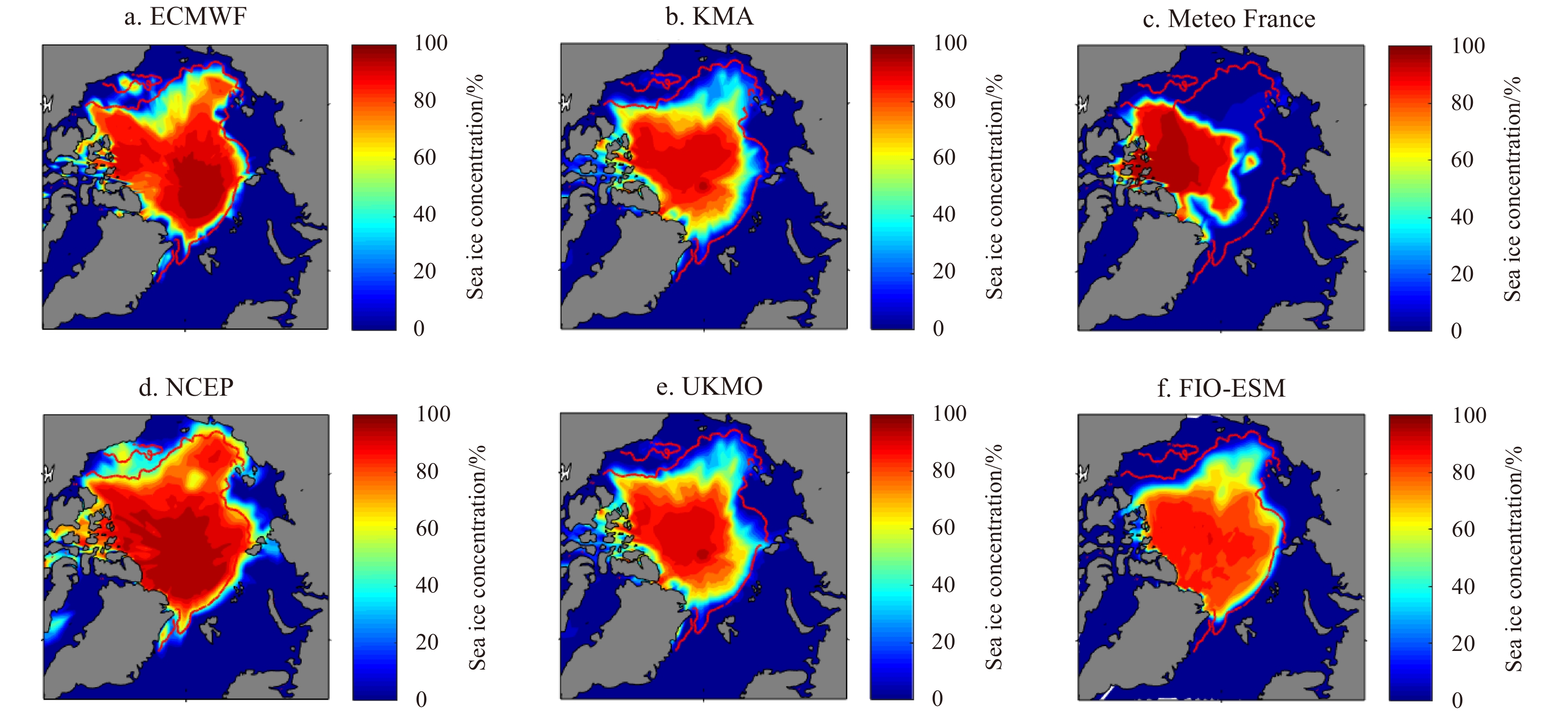
12.
Forecasted Arctic sea ice concentration for 25 August 2018 based on different forecasting systems. They are the forecasts from the early of August 2018. The red line is the sea ice edge from satellite observations.
Figure
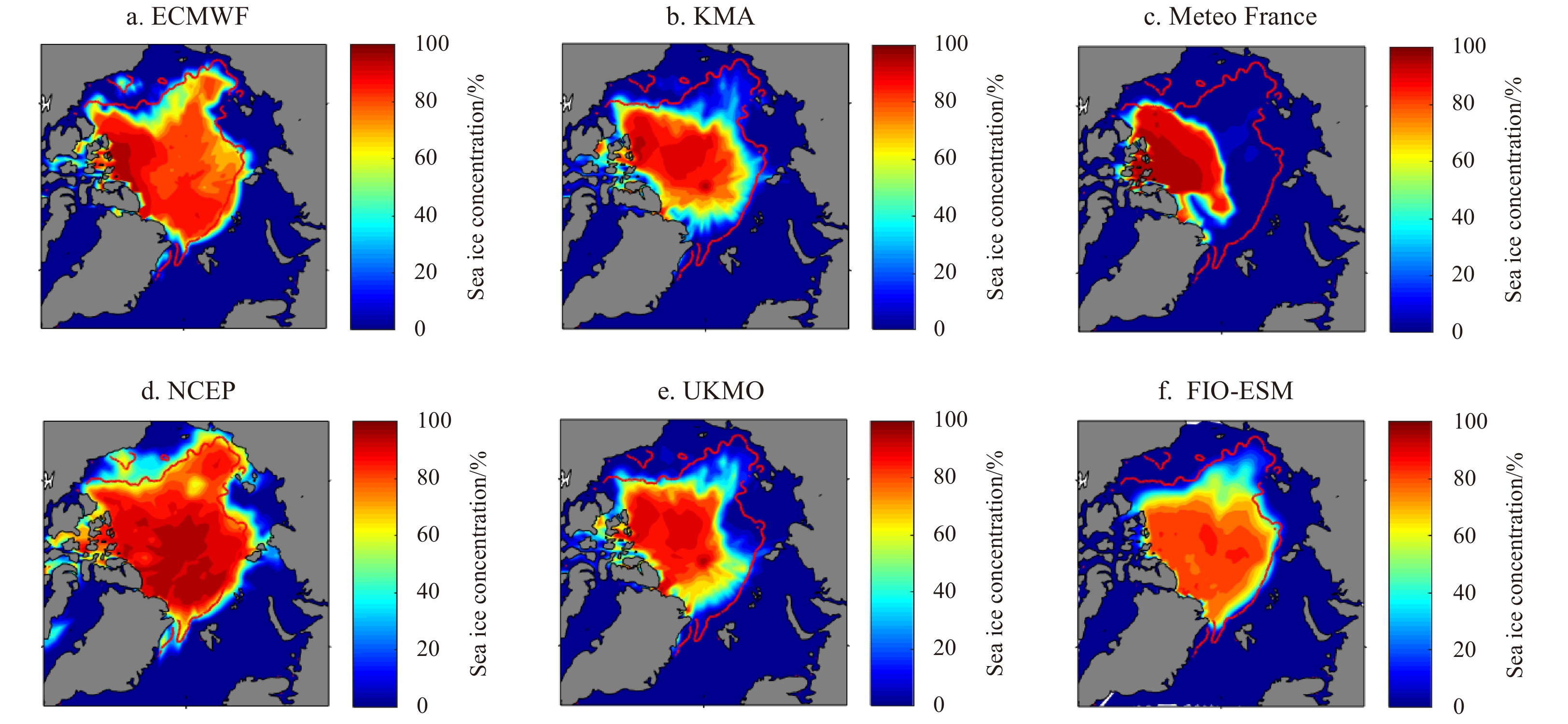
11.
Forecasted Arctic sea ice concentration for 15 August 2018 based on different forecasting systems. They are the forecasts from the early of August 2018. The red line is the sea ice edge from satellite observations.
In this study, the role of Arctic sea ice data assimilation in the FIO-ESM climate forecast system is examined. The assimilation method used here is the ensemble-based local error subspace transform Kalman filter (LESTKF). Three experiments are conducted using this climate forecast system. The first one has no sea ice data assimilation. In the second assimilation experiment, only satellite-derived sea ice concentration is assimilated. Both satellite-derived sea ice concentration and PIOMAS modelled sea ice thickness are assimilated in the third one. Each experiment has five-year (2014–2018) reanalysis simulations. Model results assessment indicates that the model biases of ice concentration, ice extent, ice volume, and ice thickness are reduced dramatically by sea ice assimilation using LESTKF. Ice concentration assimilation can help to improve ice concentration and sea ice extent simulation. All the biases of modeled ice concentration, sea ice extent, ice volume, and ice thickness can be reduced dramatically through ice concentration and thickness assimilation. So LESTKF is an effective method for FIO-ESM to improve its sea ice simulations.
Using the initializations from the three assimilation experiments, 2-month near-real-time Arctic sea ice forecasts in August 2018 were conducted for the ninth Chinese National Arctic Research Expedition. The forecast skills were assessed by comparing with the six near-real-time forecast results from subseasonal-to-seasonal (S2S) Prediction Project and the observations. The results show that ice data assimilation using LESTKF can improve the Arctic sea ice forecast skill significantly in the FIO-ESM climate forecast system. The Arctic integrated ice edge error (IIEE) is reduced by about 1/3 in this two-month near-real-time forecast by LESTKF ice assimilation, and FIO-ESM climate forecast system has relatively high Arctic sea ice forecast skill in this Arctic sea ice forecast.
The sea ice thickness dataset assimilated in this study is from PIOMAS. It belongs to modelled ice thickness but not observations. Although its winter ice volume is low compared with CryoSat-2 estimates (Laxon et al., 2013; Tilling et al., 2016), this study indicates that the long-lead forecast skill with PIOMAS sea ice thickness assimilation is higher than that without any ice thickness assimilation. So PIOMAS dataset can be used in ice thickness assimilation, especially in summer time, when there is no satellite observed basin-scale ice thickness. Considering the products of satellite observed basin-scale ice thickness usually have relatively long delay time to release, PIOMAS is a good option for sea ice thickness assimilation in the near-real-time Arctic sea ice seasonal predictions.
A limitation of this study is that only one near-real-time summer Arctic sea ice forecast was studied. The forecast skill given here may vary for different years. So more near-real-time forecast should be conducted in the following years to further study the Arctic sea ice forecast skill in the FIO-ESM climate forecast system.
Acknowledgements
Sea ice concentration products used in this paper are from EUMETSAT OSI SAF (http://osisaf.met.no) and the NSIDC (http://nsidc.org/data/seaice/). PIOMAS sea ice thickness is provided by the Polar Science Center at the University of Washington (http://psc.apl.uw.edu/research/projects/arctic-sea-ice-volume-anomaly/data/model_grid). Observed sea ice extent is from ftp://sidads.colorado.edu/DATASETS/NOAA/G02135/. Operation IceBridge sea ice thickness is from https://nsidc.org/data/NSIDC-0708/versions/1. Satellite observed sea ice thickness product is from http://data.seaiceportal.de/gallery/index_new.php. Near-real-time S2S sea ice forecasts are provided by http://www.s2sprediction.net/. The numerical experiments were conducted in the Center for High Performance Computing and System Simulation, Pilot National Laboratory for Marine Science and Technology (Qingdao). We thank the above data and computing resource providers.
Allard R A, Farrell S L, Hebert D A, et al. 2018. Utilizing CryoSat-2 sea ice thickness to initialize a coupled ice-ocean modeling system. Advances in Space Research, 62(6): 1265–1280. doi: 10.1016/j.asr.2017.12.030
[2]
Barber D G, Hop H, Mundy C J, et al. 2015. Selected physical, biological and biogeochemical implications of a rapidly changing Arctic Marginal Ice Zone. Progress in Oceanography, 139: 122–150. doi: 10.1016/j.pocean.2015.09.003
[3]
Blockley E W, Peterson K A. 2018. Improving Met Office seasonal predictions of Arctic sea ice using assimilation of CryoSat-2 thickness. The Cryosphere, 12(11): 3419–3438. doi: 10.5194/tc-12-3419-2018
[4]
Cavalieri D J, Parkinson C L, Gloersen P, et al. 1996. Sea ice concentrations from Nimbus-7 SMMR and DMSP SSM/I-SSMIS passive microwave data version 1. Boulder, CO, USA: NASA DAAC at the National Snow and Ice Data Center
[5]
Chen Zhiqiang, Liu Jiping, Song Mirong, et al. 2017. Impacts of assimilating satellite sea ice concentration and thickness on Arctic sea ice prediction in the NCEP climate forecast system. Journal of Climate, 30(21): 8429–8446. doi: 10.1175/JCLI-D-17-0093.1
[6]
Chen Hui, Yin Xunqiang, Bao Ying, et al. 2016. Ocean satellite data assimilation experiments in FIO-ESM using ensemble adjustment Kalman filter. Science China Earth Sciences, 59(3): 484–494. doi: 10.1007/s11430-015-5187-2
[7]
Chevallier M, Salas-Mélia D. 2012. The role of sea ice thickness distribution in the Arctic sea ice potential predictability: a diagnostic approach with a coupled GCM. Journal of Climate, 25(8): 3025–3038. doi: 10.1175/JCLI-D-11-00209.1
[8]
Cohen J, Screen J A, Furtado J C, et al. 2014. Recent Arctic amplification and extreme mid-latitude weather. Nature Geoscience, 7(9): 627–637. doi: 10.1038/ngeo2234
[9]
Collins W D, Rasch P J, Boville B A, et al. 2006. The formulation and atmospheric simulation of the Community Atmosphere Model Version 3 (CAM3). Journal of Climate, 19(11): 2144–2161. doi: 10.1175/jcli3760.1
[10]
Collow T W, Wang Wanqiu, Kumar A, et al. 2015. Improving Arctic sea ice prediction using PIOMAS initial sea ice thickness in a coupled ocean–atmosphere model. Monthly Weather Review, 143(11): 4618–4630. doi: 10.1175/MWR-D-15-0097.1
[11]
Day J J, Hawkins E, Tietsche S. 2014. Will Arctic sea ice thickness initialization improve seasonal forecast skill?. Geophysical Research Letters, 41(21): 7566–7575. doi: 10.1002/2014GL061694
[12]
Dickinson R E, Oleson K W, Bonan G, et al. 2006. The community land model and its climate statistics as a component of the community climate system model. Journal of Climate, 19(11): 2302–2324. doi: 10.1175/JCLI3742.1
[13]
Ducet N, Le Traon P Y, Reverdin G. 2000. Global high-resolution mapping of ocean circulation from TOPEX/Poseidon and ERS-1 and -2. Journal of Geophysical Research: Oceans, 105(C8): 19477–19498. doi: 10.1029/2000jc900063
[14]
Fetterer F, Knowles K, Meier W, et al. 2017. Sea ice index, version 3. Boulder, CO, USA: National Snow and Ice Data Center, doi: 10.7265/N5K072F8
[15]
Fowler C, Emery W J, Maslanik J. 2004. Satellite-derived evolution of Arctic sea ice age: October 1978 to March 2003. IEEE Geoscience and Remote Sensing Letters, 1(2): 71–74. doi: 10.1109/LGRS.2004.824741
[16]
Goessling H F, Tietsche S, Day J J, et al. 2016. Predictability of the Arctic sea ice edge. Geophysical Research Letters, 43(4): 1642–1650. doi: 10.1002/2015GL067232
[17]
Hakkinen S, Proshutinsky A, Ashik I. 2008. Sea ice drift in the Arctic since the 1950s. Geophysical Research Letters, 35(19): L19704. doi: 10.1029/2008GL034791
[18]
Hebert D A, Allard R A, Metzger E J, et al. 2015. Short-term sea ice forecasting: an assessment of ice concentration and ice drift forecasts using the U.S. Navy’s Arctic Cap Nowcast/Forecast System. Journal of Geophysical Research: Oceans, 120(12): 8327–8345. doi: 10.1002/2015JC011283
[19]
Hunke E C, Lipscomb W H. 2008. CICE: the Los Alamos sea ice model. documentation and software user’s manual Version 4.0, LA-CC-06-012. Los Alamos, NM, USA: Los Alamos National Laboratory
[20]
Kimmritz M, Counillon F, Bitz C M, et al. 2018. Optimising assimilation of sea ice concentration in an Earth system model with a multicategory sea ice model. Tellus A: Dynamic Meteorology and Oceanography, 70(1): 1–23. doi: 10.1080/16000870.2018.1435945
[21]
Kwok R, Cunningham G F. 2015. Variability of Arctic sea ice thickness and volume from CryoSat-2. Philosophical Transactions of the Royal Society A: Mathematical, 373(2045): 20140157. doi: 10.1098/rsta.2014.0157
[22]
Kwok R, Rothrock D A. 2009. Decline in Arctic sea ice thickness from submarine and ICESat records: 1958–2008. Geophysical Research Letters, 36(15): L15501. doi: 10.1029/2009GL039035
[23]
Laxon S W, Giles K A, Ridout A L, et al. 2013. CryoSat-2 estimates of Arctic sea ice thickness and volume. Geophysical Research Letters, 40(4): 732–737. doi: 10.1002/grl.50193
[24]
Lemieux J F, Beaudoin C, Dupont F, et al. 2016. The Regional Ice Prediction System (RIPS): verification of forecast sea ice concentration. Quarterly Journal of the Royal Meteorological Society, 142(695): 632–643. doi: 10.1002/qj.2526
[25]
Lindsay R, Haas C, Hendricks S, et al. 2012. Seasonal forecasts of Arctic sea ice initialized with observations of ice thickness. Geophysical Research Letters, 39(21): L21502. doi: 10.1029/2012GL053576
[26]
Lindsay R, Schweiger A. 2015. Arctic sea ice thickness loss determined using subsurface, aircraft, and satellite observations. The Cryosphere, 9(1): 269–283. doi: 10.5194/tc-9-269-2015
[27]
Lindsay R W, Zhang J. 2006. Assimilation of ice concentration in an ice–ocean model. Journal of Atmospheric and Oceanic Technology, 23(5): 742–749. doi: 10.1175/jtech1871.1
[28]
Lisæter K A, Evensen G, Laxon S. 2017. Assimilating synthetic CryoSat sea ice thickness in a coupled ice-ocean model. Journal of Geophysical Research: Oceans, 112(C7): C07023. doi: 10.1029/2006JC003786
[29]
Lisæter K A, Rosanova J, Evensen G. 2003. Assimilation of ice concentration in a coupled ice–ocean model, using the Ensemble Kalman filter. Ocean Dynamics, 53(4): 368–388. doi: 10.1007/s10236-003-0049-4
[30]
Liu Jiping, Chen Zhiqiang, Hu Yongyun, et al. 2019. Towards reliable Arctic sea ice prediction using multivariate data assimilation. Science Bulletin, 64(1): 63–72. doi: 10.1016/j.scib.2018.11.018
[31]
Liu Jiping, Curry J A, Wang Huijun, et al. 2012. Impact of declining Arctic sea ice on winter snowfall. Proceedings of the National Academy of Sciences of the United States of America, 109(11): 4074–4079. doi: 10.1073/pnas.1114910109
[32]
Maslanik J, Stroeve J, Fowler C, et al. 2011. Distribution and trends in Arctic sea ice age through spring 2011. Geophysical Research Letters, 38(13): L13502. doi: 10.1029/2011GL047735
[33]
Melia N, Haines K, Hawkins E. 2016. Sea ice decline and 21st century trans-Arctic shipping routes. Geophysical Research Letters, 43(18): 9720–9728. doi: 10.1002/2016GL069315
[34]
Mori M, Watanabe M, Shiogama H, et al. 2014. Robust Arctic sea-ice influence on the frequent Eurasian cold winters in past decades. Nature Geoscience, 7(12): 869–873. doi: 10.1038/ngeo2277
[35]
Mu Longjiang, Yang Qinghua, Losch M, et al. 2018. Improving sea ice thickness estimates by assimilating CryoSat-2 and SMOS sea ice thickness data simultaneously. Quarterly Journal of the Royal Meteorological Society, 144(711): 529–538. doi: 10.1002/qj.3225
[36]
Nerger L, Hiller W. 2013. Software for ensemble-based data assimilation systems—Implementation strategies and scalability. Computers&Geosciences, 55: 110–118. doi: 10.1016/j.cageo.2012.03.026
[37]
Nghiem S V, Rigor I G, Perovich D K, et al. 2007. Rapid reduction of Arctic perennial sea ice. Geophysical Research Letters, 34(19): L19504. doi: 10.1029/2007GL031138
[38]
Olason E, Notz D. 2014. Drivers of variability in Arctic sea-ice drift speed. Journal of Geophysical Research: Oceans, 119(9): 5755–5775. doi: 10.1002/2014JC009897
[39]
Parkinson C L. 2019. A 40-y record reveals gradual Antarctic sea ice increases followed by decreases at rates far exceeding the rates seen in the Arctic. Proceedings of the National Academy of Sciences of the United States of America, 116(29): 14414–14423. doi: 10.1073/pnas.1906556116
[40]
Parkinson C L, Cavalieri D J. 2008. Arctic sea ice variability and trends, 1979–2006. Journal of Geophysical Research, 113(C7): C07003. doi: 10.1029/2007JC004558
[41]
Qiao Fangli, Song Zhenya, Bao Ying, et al. 2013. Development and evaluation of an Earth System Model with surface gravity waves. Journal of Geophysical Research: Oceans, 118(9): 4514–4524. doi: 10.1002/jgrc.20327
[42]
Qiao Fangli, Yuan Yeli, Yang Yongzeng, et al. 2004. Wave-induced mixing in the upper ocean: distribution and application to a global ocean circulation model. Geophysical Research Letters, 31(11): L11303. doi: 10.1029/2004GL019824
[43]
Reynolds R W, Smith T M, Liu Chunying, et al. 2007. Daily high-resolution-blended analyses for sea surface temperature. Journal of Climate, 20(22): 5473–5496. doi: 10.1175/2007JCLI1824.1
[44]
Ricker R, Hendricks S, Kaleschke L, et al. 2017. A weekly Arctic sea-ice thickness data record from merged CryoSat-2 and SMOS satellite data. The Cryosphere, 11(4): 1607–1623. doi: 10.5194/tc-11-1607-2017
[45]
Sakov P, Counillon F, Bertino L, et al. 2012. TOPAZ4: an ocean-sea ice data assimilation system for the North Atlantic and Arctic. Ocean Science, 8(4): 633–656. doi: 10.5194/os-8-633-2012
[46]
Sévellec F, Fedorov A V, Liu Wei. 2017. Arctic sea-ice decline weakens the Atlantic Meridional Overturning Circulation. Nature Climate Change, 7(8): 604–610. doi: 10.1038/nclimate3353
[47]
Schweiger A, Lindsay R, Zhang Jinlun, et al. 2011. Uncertainty in modeled Arctic sea ice volume. Journal of Geophysical Research: Oceans, 116(C8): C00D06. doi: 10.1029/2011JC007084
[48]
Shu Qi, Qiao Fangli, Bao Ying, et al. 2015. Assessment of Arctic sea ice simulation by FIO-ESM based on data assimilation experiment. Haiyang Xuebao (in Chinese), 37(11): 33–40. doi: 10.3969/j.issn.0253-4193.2015.11.004
[49]
Smith R, Jones P, Briegleb B P, et al. 2010. The Parallel Ocean Program (POP) reference manual: ocean component of the community climate system model (CCSM). Boulder, CO, USA: National Centre for Atmosphere Research
[50]
Smith L C, Stephenson S R. 2013. New Trans-Arctic shipping routes navigable by midcentury. Proceedings of the National Academy of Sciences of the United States of America, 110(13): E1191–E1195. doi: 10.1073/pnas.1214212110
[51]
Song Zhenya, Shu Qi, Bao Ying, et al. 2015. The prediction on the 2015/16 El Niño event from the perspective of FIO-ESM. Acta Oceanologica Sinica, 34(12): 67–71. doi: 10.1007/s13131-015-0787-4
[52]
Stroeve J, Hamilton L C, Bitz C M, et al. 2014. Predicting September sea ice: ensemble skill of the SEARCH sea ice outlook 2008–2013. Geophysical Research Letters, 41(7): 2411–2418. doi: 10.1002/2014GL059388
[53]
Tietsche S, Notz D, Jungclaus J H, et al. 2013. Assimilation of sea-ice concentration in a global climate model–physical and statistical aspects. Ocean Science, 9(1): 19–36. doi: 10.5194/os-9-19-2013
[54]
Tilling R L, Ridout A, Shepherd A. 2016. Near-real-time Arctic sea ice thickness and volume from CryoSat-2. The Cryosphere, 10(5): 2003–2012. doi: 10.5194/tc-10-2003-2016
[55]
Tomas R A, Deser C, Sun Lantao. 2016. The role of ocean heat transport in the global climate response to projected Arctic Sea ice loss. Journal of Climate, 29(19): 6841–6859. doi: 10.1175/JCLI-D-15-0651.1
[56]
Toyoda T, Fujii Y, Yasuda T, et al. 2016. Data assimilation of sea ice concentration into a global ocean–sea ice model with corrections for atmospheric forcing and ocean temperature fields. Journal of Oceanography, 72(2): 235–262. doi: 10.1007/s10872-015-0326-0
[57]
Wang Wanqiu, Chen Mingyue, Kumar A. 2013a. Seasonal prediction of Arctic sea ice extent from a coupled dynamical forecast system. Monthly Weather Review, 141(4): 1375–1394. doi: 10.1175/MWR-D-12-00057.1
[58]
Wang Keguang, Debernard J, Sperrevik A K, et al. 2013b. A combined optimal interpolation and nudging scheme to assimilate OSISAF sea-ice concentration into ROMS. Annals of Glaciology, 54(62): 8–12. doi: 10.3189/2013AoG62A138
[59]
Wayand N E, Bitz C M, Blanchard-Wrigglesworth E. 2019. A year-round subseasonal-to-seasonal sea ice prediction portal. Geophysical Research Letters, 46(6): 3298–3307. doi: 10.1029/2018GL081565
[60]
Xie Jiping, Counillon F, Bertino L, et al. 2016. Benefits of assimilating thin sea ice thickness from SMOS into the TOPAZ system. The Cryosphere, 10(6): 2745–2761. doi: 10.5194/tc-10-2745-2016
[61]
Yang Qinghua, Losa S N, Losch M, et al. 2014. Assimilating SMOS sea ice thickness into a coupled ice-ocean model using a local SEIK filter. Journal of Geophysical Research: Oceans, 119(10): 6680–6692. doi: 10.1002/2014JC009963
[62]
Yang Qinghua, Losa S N, Losch M, et al. 2015. Assimilating summer sea-ice concentration into a coupled ice-ocean model using a LSEIK filter. Annals of Glaciology, 56(69): 38–44. doi: 10.3189/2015AoG69A740
[63]
Yang Qinghua, Losch M, Losa S N, et al. 2016. Brief communication: the challenge and benefit of using sea ice concentration satellite data products with uncertainty estimates in summer sea ice data assimilation. The Cryosphere, 10(2): 761–774. doi: 10.5194/tc-10-761-2016
[64]
Yang Yongzeng, Qiao Fangli, Zhao Wei, et al. 2005. MASNUM ocean wave numerical model in spherical coordinates and its application. Haiyang Xuebao (in Chinese), 27(2): 1–7. doi: 10.3321/j.issn:0253-4193.2005.02.001
[65]
Yin Xunqiang. 2015. Development of assimilation module for ensemble adjustment Kalman filter and its application in ocean and climate models (in Chinese)[dissertation]. Qingdao: Ocean University of China
[66]
Zampieri L, Goessling H F, Jung T. 2018. Bright prospects for Arctic sea ice prediction on subseasonal time scales. Geophysical Research Letters, 45(18): 9731–9738. doi: 10.1029/2018GL079394
[67]
Zhang Jinlun, Ashjian C, Campbell R, et al. 2015. The influence of sea ice and snow cover and nutrient availability on the formation of massive under-ice phytoplankton blooms in the Chukchi Sea. Deep-Sea Research Part II: Topical Studies in Oceanography, 118: 122–135. doi: 10.1016/j.dsr2.2015.02.008
[68]
Zhang Jinlun, Rothrock D A. 2003. Modeling global sea ice with a thickness and enthalpy distribution model in generalized curvilinear coordinates. Monthly Weather Review, 131(5): 845–861. doi: 10.1175/1520-0493(2003)131<0845:MGSIWA>2.0.CO;2
[69]
Zhang Jinlun, Thomas D R, Rothrock D A, et al. 2003. Assimilation of ice motion observations and comparisons with submarine ice thickness data. Journal of Geophysical Research: Oceans, 108(C6): 3170. doi: 10.1029/2001JC001041
Chao Min, Qinghua Yang, Hao Luo, et al. Improving Arctic Sea-Ice Thickness Estimates with the Assimilation of CryoSat-2 Summer Observations. Ocean-Land-Atmosphere Research, 2023, 2 doi:10.34133/olar.0025
2.
Lin Huang, Yubao Qiu, Yang Li, et al. DynIceData: a gridded ice–water classification dataset at short-time intervals based on observations from multiple satellites over the marginal ice zone. Big Earth Data, 2023. doi:10.1080/20964471.2023.2230714
3.
Ying Zhang, Jinliang Hou, Chunlin Huang. Basin Scale Soil Moisture Estimation with Grid SWAT and LESTKF Based on WSN. Sensors, 2023, 24(1): 35. doi:10.3390/s24010035
4.
Qiuli Shao, Qi Shu, Bin Xiao, et al. Arctic Sea Ice Concentration Assimilation in an Operational Global 1/10° Ocean Forecast System. Remote Sensing, 2023, 15(5): 1274. doi:10.3390/rs15051274
Figure 1. Ensemble spread (one standard deviation) of simulated sea ice concentration (a–d) and sea ice thickness (e–h) on the first day of March (a, e), June (b, f), September (c, g), and December (d, h) 2014 in the FIO-ESM climate forecast system.
Figure 2. Numerical experiment processes.
Figure 3. Arctic sea ice extent (SIE) biases during 2014 to 2018. Blue, red and yellow lines are from EXP1, EXP2 and EXP3, respectively. The biases are the results between simulations and observations from NSIDC.
Figure 4. Arctic sea ice concentration observations from NSIDC (a, e) and model biases (b–d and f–h) in March (a–d) and September (e–h) during 2014 to 2018.
Figure 5. Root mean square error (RMSE) of Arctic sea ice concentration during 2014 to 2018. a, b, and c are from EXP1, EXP2, and EXP3, respectively.
Figure 6. Arctic sea ice volume (SIV) during 2014 to 2018 in the PIOMAS, EXP1, EXP2, and EXP3.
Figure 7. Root mean square error (RMSE) of winter season Arctic sea ice thickness during 2014 to 2018. a–c are calculated based on the CryoSat-2 and SMOS (CS2SMOS) merged sea ice thickness. d–f are calculated based on PIOMAS sea ice thickness.
Figure 8. Location of IceBridge observations during 2014–2018 (a) and the probability density function (PDF) distribution of modeled sea ice thickness biases compared with IceBridge observations in EXP1, EXP2, and EXP3 (b). The legend in a is the time of the observations.
Figure 9. Time series of spatial correlation coefficients between PIOMAS and modeled Arctic sea ice thickness during 2014 to 2018. Blue, red and yellow lines are for EXP1, EXP2 and EXP3, respectively.
Figure 10. Arctic integrated ice edge error (IIEE) from different near-real-time forecasts in the early of August 2018. Observation persistence represents observation-based benchmark based on the observed sea ice conditions in 1 August 2018. Climatology represents the climatology-based benchmark based on the observed sea ice conditions during 1989–2018. The observations are from the same datasets used in data assimilation. CMA represents China Meteorological Administration. ECMWF represents European Centre for Medium-Range Weather Forecasts. KMA represents Korea Meteorological Administration. Meteo France represents Météo France. NCEP represents National Centers for Environmental Prediction. UKMO represents UK Met Office. MMM represents multimodel ensemble mean. FIO-ESM EXP1, FIO-ESM EXP2, and FIO-ESM EXP3 represent the forecasts based on EXP1, EXP2 and EXP3 in this study, respectively.
Figure 12. Forecasted Arctic sea ice concentration for 25 August 2018 based on different forecasting systems. They are the forecasts from the early of August 2018. The red line is the sea ice edge from satellite observations.
Figure 11. Forecasted Arctic sea ice concentration for 15 August 2018 based on different forecasting systems. They are the forecasts from the early of August 2018. The red line is the sea ice edge from satellite observations.


 DownLoad:
 DownLoad:


 DownLoad: