Figure
1.
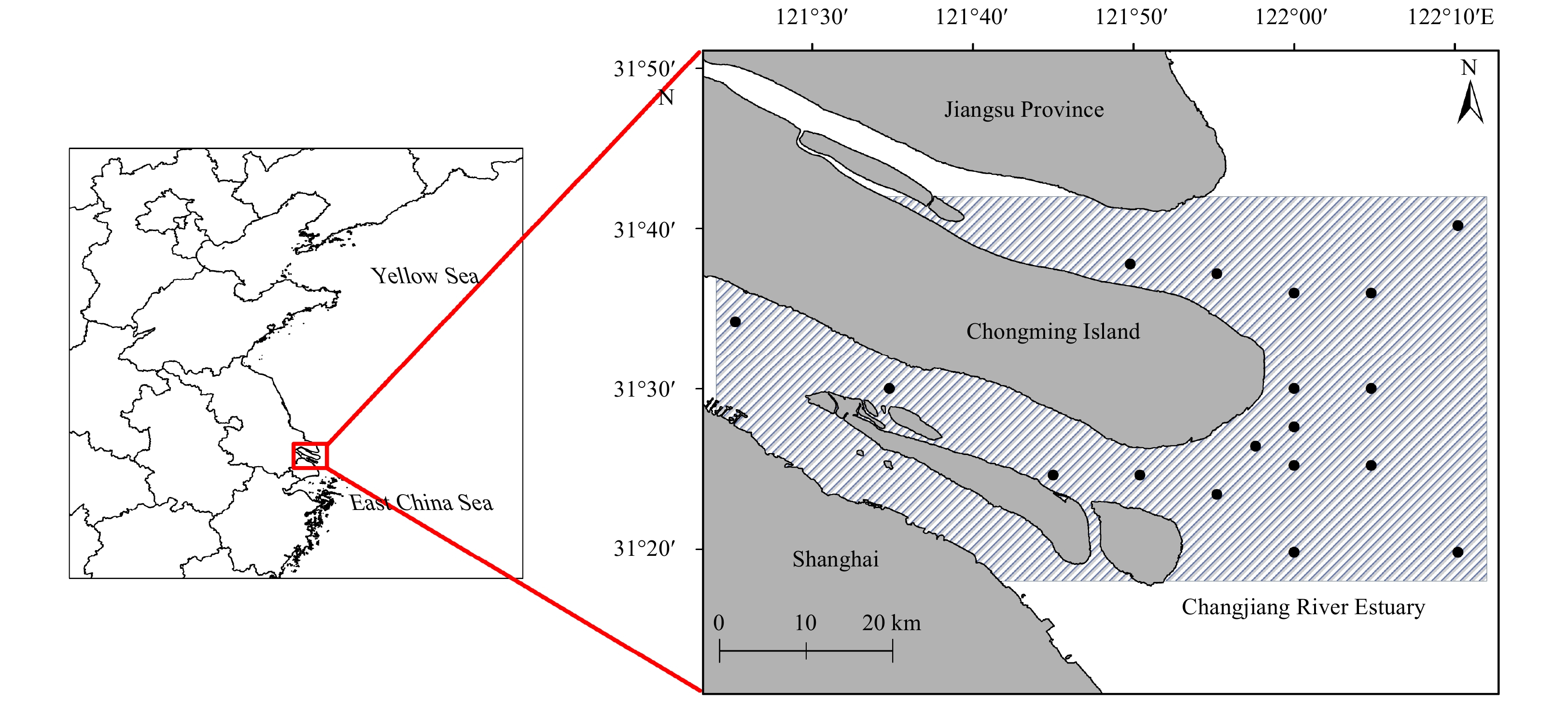
Spatial distribution of survey stations in the Changjiang River Estuary.
| Citation: | Shaoyuan Pan, Siquan Tian, Xuefang Wang, Libin Dai, Chunxia Gao, Jianfeng Tong. Comparing different spatial interpolation methods to predict the distribution of fishes: A case study of Coilia nasus in the Changjiang River Estuary[J]. Acta Oceanologica Sinica, 2021, 40(8): 119-132. doi: 10.1007/s13131-021-1789-z

|
Fish spatial distribution is important to understand for stock assessment and management (Chang et al., 2010; Li et al., 2017b; Wang et al., 2018). The aggregation and distribution of fishes are determined by their complex responses to environmental and biotic factors (Gibson et al., 1996; Zhao et al., 2014). Their preference for various combinations of environmental variables factors determine the changes in fish community structure and overall abundance (Pessanha and Araújo, 2003; Selleslagh and Amara, 2008; Ribeiro et al., 2006). The careful selection of these variables is very important when species distribution model were used to fit the relationship between abundance and environmental variables (Ma et al., 2020). Thus, it is necessary to obtain and process the appropriate environmental information of fish habitat to accurately predict its spatial distribution.
In conventional marine surveys, environment variables are usually measured at stationary stations at discreet time points, resulting in fragmented dataset or lack of continuous time-series information of certain environmental parameters. To augment limited data associated with stationary sampling designs, Spatial interpolation methods (SIMs) can use the values of known points to estimate the values of unknown points (Mueller et al, 2004). Generally, SIMs can be applied under the following circumstances: (1) the spatial resolution and pixel size of existing data do not meet the requirements; (2) the existing data model of continuous surface is inconsistent with the required data for the model; and (3) the existing data cannot completely cover the required survey area (Li and Heap, 2014; Rufino et al., 2019). SIMs have apparent advantages and use in the analysis and characterization of large-scale environmental variables, and they are one of the most effective methods to obtain a more holistic view of the continuous distribution of environmental parameters (Auchincloss et al., 2012; Rufo et al., 2018).
Different SIMs have been widely used in the analysis of the spatial distribution of fishery resources, such as that of inverse distance weight (IDW), ordinary Kriging (OK) and radial basis function (RBF). For example, Rivoirard and Wieland (2001) compared the effects of two Kriging in estimating the abundance estimation of juvenile haddock by directly interpolating the abundance data from the North Sea. Their results pointed out that the external drift Kriging (EDK) could well compensate for the effect of the daylight effect in the abundance estimation of haddock, and EDK is better than OK on the survey-based abundance index calculation. Chen et al. (2016) on the other hand used IDW, global polynomial interpolation (GPI), local polynomial interpolation (LPI) and OK to estimate the abundance and compared the effects of these SIMs on determining the fishery resources density in the Yellow Sea. Considering feasibility and accuracy, IDW was suggested as an effective routine method. Diaconu et al. (2019) compared the effects of SIMs in the analysis of bathymetric measurements and found that the estimated results affected the accuracy of the final bathymetric maps. Rufino et al. (2019) studied the effects of SIMs in estimating species distribution, and recommended that the hypotheses of methods must be declared before interpolating indicators (i.e., index of aggregation, percentage of presence, center of gravity, inertia and isotropy), especially when the indicators are to be compared among different studies. Thus, the optimal interpolation was needed depending on the need or application as reported in different studies, and that various hypotheses of methods may affect the estimation results of estimating spatial distribution of environmental and biotic factors (Li and Heap, 2008, 2011; Li et al., 2011).
As the largest estuary in China, the Changjiang River Estuary (CRE) is an important place for the growth, reproduction, and breeding of many migratory fishes due to its complex and dynamic ecosystems (Shan et al., 2017). Coilia nasus is an important fish with high economic value in the CRE, and its spatial distribution is closely related to different environmental factors such as water temperature, water depth, pH, chlorophyll a and salinity (Tong et al., 2018; Ma et al., 2020). Here, this study compared the effects of different SIMs on the estimation of environmental variables and the effects of estimated values on the predicted spatial distribution of Coilia nasus. The goal is to provide a case study for determining the optimal SIMs of continuous environmental factors of fish habitat in the CRE.
Data were collected during the routine monitoring of fishery resources conducted by the Chinese sturgeon nature reserve in the CRE from 2012 to 2014. Surveys were conducted in the spring (May), summer (August), autumn (November) and winter (February) throughout the survey period following a stationary sampling design. Data used in this study were obtained from 18 stations in the CRE (Fig. 1). The bottom trawl used for sampling had a net wideness of 6 m, cod end mesh size was 2 cm, height was 2 m and width was 6 m. One tow was performed at each station at a speed of 2 n mile/h for 15 min.
For all of the fish species harvested using the bottom trawl, their length, weight, and capture time were recorded. Also, environmental variables such as water depth (Depth, m), bottom water temperature (Temp, °C), bottom salinity (Salinity, 10−12), pH and dissolved oxygen (DO, mg/L) were measured using a multi-parameter water quality meter (WTW-3430). Variables such as chlorophyll a (Chl a, μg/L) and chemical oxygen demand (COD, mg/L) at each site were obtained by analyzing water samples in the laboratory.
Predictive variables measured in this study were divided into spatio-temporal and environmental factors. Spatio-temporal factors included season, longitude and latitude, and environmental factors included Depth, Temp, salinity, DO, pH, Chl a and COD. Strong correlation between environmental variables will result in multicollinearity, which often leads to the model overfitting, low accuracy of prediction, and uncertainty of variable selection in modeling (Zhao et al., 2014). Correlation analysis and variance inflation factors (VIFs) were used to judge for multicollinearity of variables before spatial interpolation (Liu et al., 2019), and those environmental variables with VIF>3 in the model were removed (Thomson and Emery, 2014; Sagarese et al., 2014).
In this study, IDW, OK and RBF were used to interpolate environmental variables. The OK approach included three semivariogram models namely exponential (OKE), gaussian (OKG) and spherical (OKS). The RBF model is comprised of the regularized spline function (RS) and the tension spline function (TS).
SIMs have different assumptions and potentially suitable data sets. IDW assumes that the unknown points are more easily influenced by the known points in the closer distance than those from afar (Shepard, 1968). All estimated values of IDW fall between the known maximum and minimum values, and the main factor influencing the accuracy of IDW is the exponential power value (Foehn et al., 2018).
OK assumes that the variables involved are random but spatially correlated to some extent (Coburn, 2000). OK focuses on spatially related factors and directly interpolates them with the fitted semi-variances which were calculated by semivariogram models. During the calculation, not only the influence of the distance between interpolated points are considered, but also the position and the overall spatial distribution of the known points. The weight used in the OK related to the semi-variances between the interpolation point to the known point and among the known points (Vicente-Serrano et al., 2003). This makes the OK model different from IDW.
RBF uses a basis function to determine the weight of the known points and to create a surface with minimum total curvature, which can also capture the overall trend and obtain local changes (Johnston et al., 2001). The basis function determines the matching of the surface and interpolated points (Bhunia et al., 2018). The RS (Mitášová and Mitáš, 1993) generates a smooth and graded surface, but the interpolation results may be out of the value range of the known points. The TS (Mitáš and Mitášová, 1988) adjusts the hardness of the surface according to the fitted surface, and the interpolated results then become closer to the value range of the known points.
For more details on the algorithms for each interpolation method, see the article of Shen et al. (2019). In this study, the SIMs were carried out in ArcGIS 10.3 with a spatial resolution of 0.05°×0.05°.
Cross-validation was used to compare the effectiveness of SIMs. In the process of cross-validation, one of the known points is removed from the data set, and then estimated the value of the removed points by the other points. Meanwhile, the measured value is compared with the estimated value and the error is calculated (Shen et al., 2019). After completing the above steps for each point, the mean error (ME) and root mean square error (RMSE) were calculated as indices to evaluate the accuracy of the SIMs. The ME and RMSE both quantify the difference between the observed and predicted density (Stow et al., 2009). ME reflects the overall estimation bias of the SIMs (Isaaks and Srivastava, 1988). If the ME is closer to 0, then the predicted value is more unbiased. RMSE needs to be compared first because it reflects the error of estimated values and measured values. When RMSE is close to 0, this indicates that the fitting is better (Ding et al., 2018). Equations used for ME and RMSE are as follows:
| $$ \mathrm{M}\mathrm{E}=\frac{1}{n}\sum _{i=1}^{n}[{z}_{{x}_{i}}-{z}_{{x}_{i}}^{\mathrm{*}}]{\rm{,}} $$ | (1) |
| $$ \mathrm{R}\mathrm{M}\mathrm{S}\mathrm{E}=\sqrt{\frac{1}{n}\sum _{i=1}^{n}{[{z}_{{x}_{i}}-{z}_{{x}_{i}}^{*}]}^{2}}{\rm{,}} $$ | (2) |
where
A two-stage generalized additive model (GAM), which can reduce the effect of zero catches was used to establish the relationship between environmental variables and the changes of Coilia nasus resources in the CRE. The two-stage GAM assumes that the zero records indicated absence of Coilia nasus in the surveyed habitat rather than just low abundance. This approach had advantages in preserving the information of zero observations (Chang et al., 2010; Li et al., 2015). The first stage of GAM model estimated that the presence probability of Coilia nasus was a binomial error distribution, and the second stage of GAM model used a function of Gaussian error distribution to estimate the log-transformation abundance of Coilia nasus. Based on the value of the smallest corrected Akaike information criterion (AICc), the variables were selected via backward stepwise regression method (Beier, 2001). The two-stage GAM model formula is as follows:
GAM 1:
| $$ \begin{split} {{\rm{logit}}}\left(p\right)=& {\rm{year}}+{\rm{month}}+s\left({\rm{Lat}}\right)+s\left({\rm{Depth}}\right)+\\ & s\left({\rm{Temp}}\right)+s\left({\rm{Salinity}}\right)+s\left({\rm{pH}}\right)+\varepsilon{\rm{,}} \end{split} $$ | (3) |
GAM 2:
| $$ \begin{split} {{\rm{ln}}}\;(d)=& {\rm{year}}+{\rm{month}}+s({\rm{Lon}})+s({\rm{Lat}})+s({\rm{Depth}})+\\ & s({\rm{Temp}})+s({\rm{pH}})+s({\rm{Chl }}a)+\varepsilon{\rm{,}} \end{split} $$ | (4) |
where p is the presence probability of Coilia nasus, d is the abundance of Coilia nasus (unit: ind./km2), s is the spline smoothing function; Lon, Lat, Depth, Temp, Salinity, pH, Chl a are longitude, latitude, water depth (unit: m), water temperature (unit: °C), salinity (10−12), pH, chlorophyll a (unit: mg/L) respectively, and ε is the random error term.
Combining the results of the two-stage GAM, the following formula was used to estimate the total log-abundance of Coilia nasus (D):
| $$ {{\rm{ln}}}(D)=p\;{{\rm{ln}}}(d). $$ | (5) |
The area under the receiver operating characteristic curve (AUC) was used to verify the predictive ability of the first stage GAM (Hanley and McNeil, 1982). AUC ranged from 0 to 1, where AUC equals 0.5 indicates that the prediction of the model is consistent with the random prediction. When AUC is closer to 1, the probability of correct prediction of the model is higher and when AUC value is closer to 0, this indicates worse than the random prediction (Zou et al., 2007). The RMSE and R2 from the linear regression model were used to judge the fitting degree of the second stage GAM (Li et al., 2018).
Based on VIFs analysis, the values of DO and salinity were larger than 3. However, salinity was reconsidered in subsequent analysis since it is an important variable influencing changes in the spatial distribution of fish communities in most estuaries. Moreover, salinity had the highest correlation coefficient between environmental variables, particularly with COD. Because of this, DO and COD were then removed from subsequent analysis because of collinearity. The remaining variables used in next steps were Lon, Lat, Depth, Temp, Salinity, pH and Chl a, which had VIF values of 1.74, 2.38, 1.24, 1.21, 2.57, 1.31 and 1.26 respectively.
After implementing the AICc approach, the first stage GAM retained five variables including Lat, Depth, Temp, Salinity and pH. This model explained 30.1% of the deviance, and had an AUC value of 0.85, which better predicted the probabilistic presence of Coilia nasus. The second stage GAM retained six variables, namely Lon, Lat, Depth, Temp, pH, and Chl a. Model deviation accounted for 69.0% of the variance, with an R2 of 0.58 and RMSE of 324.50 (Table 1).
| Model | Deviance/% | Sample size | AUC | Variables |
| GAM1 | 30.1 | 137 | 0.85 | Lat, Depth, Temp, Salinity, pH |
| Model | Deviance/% | Sample size | RMSE | Variables |
| GAM2 | 69.0 | 48 | 324.50 | Lon, Lat, Depth, Temp, pH, Chl a |
| Note: Lon: longitude; Lat: latitude; Depth: water depth; Temp: water temperature; Chl a: chlorophyll a. | ||||
 DownLoad:
CSV
DownLoad:
CSV
The values of environmental variables estimated in CRE by various SIMs varied significantly (Table 2). The mean value of each variable was close to the measured data, while the mean values of the interpolation results of Temp, Salinity and pH were smaller than the measured data. Meanwhile, the mean values of Temp and pH were not significantly smaller than that of the measured data, and Salinity was a little higher. The standard deviation (SD) and the coefficient of variation (CV) of the interpolation results of all environmental variables were smaller than the measured data. Among them, the SD and CV of pH were the least, indicating that the degree of dispersion was also the lowest. Meanwhile, the CV of Chl a was the largest and the measures of dispersion degree were the highest. By comparing the skewness (Sk) and kurtosis (Ku), the distributions of the estimated value of the variables were consistent with the measured data after interpolation. Except for pH, the Sk of the remaining variables were larger than 0, indicating that the estimated values were positively skewed to the right, while the value of pH was skewed to the left. The Ku of Depth, pH, and Chl a were larger than 0, indicating that the estimated value distribution was steeper than the normal distribution and presented a peak distribution. Ku of Temp and Salinity were less than 0, showing a flat peak distribution.
| Methods | Depth | Temperature | |||||||||
| mean (range)/m | SD/m | CV/% | Sk | Ku | mean (range)/°C | SD/°C | CV/% | Sk | Ku | ||
| True | 6.25 (1.50–20.00) | 3.12 | 49.92 | 1.84 | 5.18 | 18.16 (5.60–30.10) | 8.04 | 44.25 | 0.06 | −1.36 | |
| OKE | 6.35 (2.66–15.40) | 1.64 | 25.83 | 1.38 | 4.07 | 18.02 (6.13–29.93) | 7.82 | 43.40 | 0.10 | −1.37 | |
| OKG | 6.39 (1.99–15.56) | 1.95 | 30.56 | 1.37 | 4.06 | 18.02 (4.82–30.37) | 7.86 | 43.62 | 0.11 | −1.37 | |
| OKS | 6.56 (2.34–15.70) | 1.70 | 25.95 | 1.07 | 2.78 | 18.01 (6.13–29.95) | 7.85 | 43.59 | 0.11 | −1.37 | |
| IDW | 6.13 (2.01–15.00) | 1.58 | 25.77 | 2.15 | 7.69 | 18.05 (5.69–30.10) | 7.87 | 43.60 | 0.09 | −1.38 | |
| RS | 6.43 (0.00–16.15) | 2.11 | 32.81 | 0.76 | 3.50 | 18.01 (5.47–30.16) | 7.82 | 43.42 | 0.10 | −1.36 | |
| TS | 6.57 (0.75–19.73) | 2.06 | 31.40 | 1.80 | 6.40 | 17.99 (5.57–30.08) | 7.86 | 43.69 | 0.09 | −1.37 | |
| Methods | Salinity | pH | |||||||||
| mean (range)/10−12 | SD/10−12 | CV/% | Sk | Ku | mean (range) | SD | CV/% | Sk | Ku | ||
| True | 9.18 (0.00–29.80) | 10.14 | 111.31 | 0.53 | −1.32 | 8.01 (6.62–9.03) | 0.39 | 4.87 | −1.35 | 3.10 | |
| OKE | 8.09 (0.00–29.50) | 7.23 | 89.48 | 0.85 | −0.32 | 8.00 (7.25–8.55) | 0.26 | 3.25 | −0.95 | 0.76 | |
| OKG | 8.42 (0.00–42.87) | 8.49 | 101.07 | 0.91 | −0.05 | 8.00 (7.14–8.55) | 0.27 | 3.38 | −1.03 | 0.95 | |
| OKS | 8.11 (0.00–30.78) | 7.80 | 96.30 | 0.81 | −0.47 | 8.01 (7.22–8.55) | 0.27 | 3.37 | −1.07 | 0.82 | |
| IDW | 7.71 (0.00–29.78) | 8.56 | 111.17 | 0.86 | −0.66 | 8.00 (6.92–8.55) | 0.28 | 3.50 | −0.94 | 0.95 | |
| RS | 7.87 (0.00–34.27) | 7.74 | 98.60 | 0.93 | −0.12 | 8.00 (6.75–8.67) | 0.28 | 3.50 | −1.14 | 1.55 | |
| TS | 7.69 (0.00–32.56) | 7.57 | 98.57 | 0.94 | −0.14 | 8.00 (6.90–8.58) | 0.28 | 3.50 | −1.08 | 1.12 | |
| Methods | Chlorophyll a | ||||||||||
| mean (range)/μg·L−1 | SD/μg·L−1 | CV/% | Sk | Ku | |||||||
| True | 1.84 (0.09–11.25) | 2.10 | 117.32 | 2.38 | 5.95 | ||||||
| OKE | 1.87 (0.12–10.95) | 2.01 | 107.47 | 1.93 | 3.01 | ||||||
| OKG | 1.90 (0.12–11.63) | 2.08 | 110.05 | 2.03 | 3.52 | ||||||
| OKS | 1.89 (0.13–11.12) | 2.05 | 108.47 | 1.95 | 3.09 | ||||||
| IDW | 1.88 (0.11–11.25) | 2.08 | 111.23 | 2.06 | 3.57 | ||||||
| RS | 1.87 (0.11–11.36) | 2.03 | 109.14 | 2.05 | 3.65 | ||||||
| TS | 1.88 (0.13–11.52) | 2.08 | 110.64 | 2.14 | 4.13 | ||||||
| Note: SD: standard deviation; CV: the coefficient of variation; Sk: skewness; Ku: kurtosis; True: measured values; OKE: Ordinary Kriging based on exponential model; OKG: Ordinary Kriging based on gaussian model; OKS: Ordinary Kriging based on spherical model; IDW: inverse distance weight; RS: Regularized Spline Function; TS; Tension Spline Function. | |||||||||||
DownLoad:
CSV
The central tendency of interpolation results also varied (Fig. 2). For example, although the estimated values of Temp, pH, and Chl a obtained by SIMs only slightly varied, they were significant (p<0.01). The upper quartile values of these three variables were all lower than the measured values, indicating that the spatial interpolation method had an impact on the central tendency of the data. As for Depth, the values varied the most when estimated with IDW. Of all the environmental variables, salinity varied the most when estimated with OKE. Different SIMs had different responses to each environmental variable, but there was no consistent trend on the estimated values being larger or smaller than the measured values.

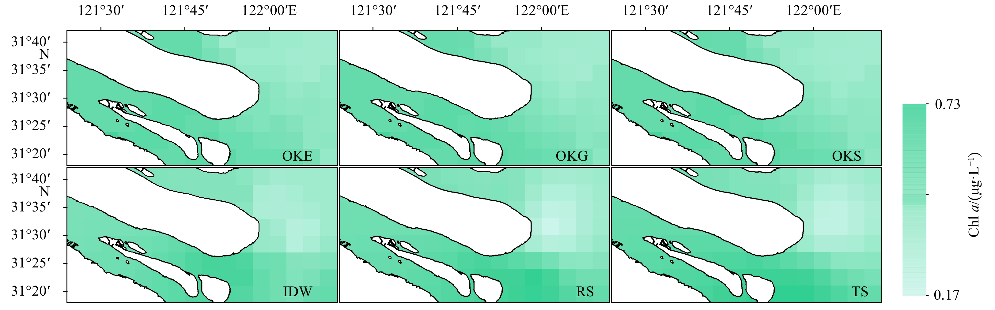
Although the estimated values of environmental variables obtained by various SIMs differed, SIMs generally still did not change the overall distribution trend of environmental variables. For example, the estimated values of Depth were higher, while pH and Chl a were lower outside the estuary (Figs S1–S15). Taking the 2014 winter environmental data in the CRE as an example, the spatial distribution maps of environmental factors were constructed (Figs 3–7). Results showed that for environmental variables with small changes in their own spatial distribution (such as Depth, Temp, pH, and Chl a), differences of the estimated values obtained by each SIMs were very small. Among them, spatial distribution of the values obtained by IDW and OK were blocky, but the spatial continuity of IDW were lower than OK. The values obtained by RBF on the other hand were generally high.


Spatial distribution of salinity significantly differed inside and outside of the CRE (Fig. 5). The estimated values of salinity obtained by OK were higher on the inside of the estuary and the continuity was lower than other methods. The three semivariogram models of OK also showed differences in the areas with higher salinity. In contrast, salinity estimated by IDW were higher than those obtained by other methods on the north side of the CRE, and the continuity was lower on the outside of the CRE. The values of RBF were the smoothest in terms of spatial distribution, while the values of the two RBF methods were very similar.
The cross-validation of the interpolations for each environmental variables showed that the optimal SIMs applicable to each variable differed (Table 3). IDW was the most suitable method for Depth and Chl a in the CRE, which had RMSE values of 3.03 and 0.46, respectively. Meanwhile, the method that well suited Temp and Salinity was RS, with observed RMSE values of 1.18 and 5.72, respectively. The applicable method for pH was OKG with observed RMSE value 0.19. Also, pH recorded the lowest RMSE value along with the lowest measures of dispersion. The maximum RMSE value of environmental variables was obtained by OKG. The ME of different interpolation results of each environmental variable was close to 0, indicating that the interpolation results were almost unbiased.
| Methods | Depth/m | Temperature /°C | Salinity/10−12 | pH | Chlorophyll a/(μg·L−1) | |||||||||
| ME | RMSE | ME | RMSE | ME | RMSE | ME | RMSE | ME | RMSE | |||||
| OKE | −0.460 | 3.251 | 0.074 | 1.262 | 0.192 | 6.245 | 0.000 | 0.200 | −0.030 | 0.510 | ||||
| OKG | −0.507 | 3.394 | 0.111 | 1.300 | −0.140 | 6.458 | 0.001 | 0.194 | −0.038 | 0.526 | ||||
| OKS | −0.485 | 3.320 | 0.085 | 1.282 | 0.016 | 6.128 | 0.000 | 0.196 | −0.031 | 0.480 | ||||
| IDW | −0.491 | 3.025 | 0.117 | 1.188 | 0.753 | 6.063 | 0.005 | 0.199 | −0.069 | 0.462 | ||||
| RS | −0.371 | 3.166 | 0.050 | 1.181 | 0.101 | 5.722 | 0.002 | 0.208 | −0.033 | 0.476 | ||||
| TS | −0.378 | 3.118 | 0.039 | 1.195 | 0.124 | 5.774 | 0.002 | 0.205 | −0.010 | 0.479 | ||||
| Note: ME: mean error; RMSE: root mean square error. The most applicable SIMs to each variable was in bold print. OKE: ordinary Kriging based on exponential model; OKG: ordinary Kriging based on Gaussian model; OKS: ordinary Kriging based on spherical model; IDW: inverse distance weight; RS: regularized spline function; TS: tension spline function. | ||||||||||||||
DownLoad:
CSV
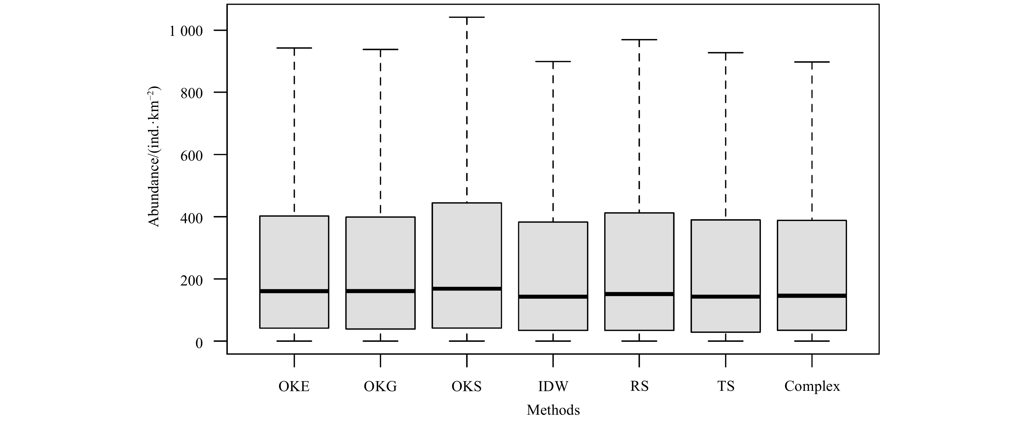
The interpolation results of environmental variables obtained by different SIMs and the results obtained by the most suitable SIMs (use Complex instead below) were used to predict the abundance of Coilia nasus in the CRE from 2012 to 2014. The mean value of the predicted abundance of Coilia nasus by each method was similar (267–293 ind./km2), but the maximum value varied significantly (1 791–2 355 ind./km2) (Table 4). Among them, the predicted mean and maximum values of IDW were the lowest, while highest mean and maximum values were obtained by OKS and TS respectively. The values and distribution trends of the predicted abundance values based on Complex were between the maximum and minimum values of the other methods. The predicted values with the greatest degree of dispersion was TS, while the smallest was with OKS (Fig. 8). Sk and Ku of all the predicted abundance values were larger than 0, indicating that the data had a positively skewed peak distribution.
| Methods | Mean (Range)/(ind.·km−2) | SD | CV/% | Sk | Ku |
| OKE | 280 (0–2227) | 328.18 | 117.21 | 2.01 | 5.61 |
| OKG | 277 (0–2257) | 327.29 | 118.16 | 2.10 | 6.31 |
| OKS | 293 (0–2277) | 336.09 | 114.71 | 1.84 | 4.72 |
| IDW | 267 (0–1791) | 320.39 | 120.00 | 1.78 | 3.31 |
| RS | 278 (0–2203) | 338.23 | 121.67 | 2.02 | 5.38 |
| TS | 272 (0–2355) | 346.36 | 127.34 | 2.27 | 7.13 |
| Complex | 268 (0–1933) | 332.86 | 124.20 | 1.87 | 4.03 |
| Note: OKE: ordinary Kriging based on exponential model; OKG: ordinary Kriging based on Gaussian model; OKS: ordinary Kriging based on spherical model; IDW: inverse distance weight; RS: regularized spline function; TS: tension spline function; Complex: the results obtained by the most suitable SIMs of environmental variables. | |||||
DownLoad:
CSV

Different SIMs obtained different estimated values of the environmental variables, which in turn will affect the predicted values of the abundance of Coilia nasus. The abundance of Coilia nasus in the winter of 2012–2014 and different seasons in 2014 of the CRE were then used as examples (Figs 9 and 10). Results showed that the spatial trend of the predicted abundance of Coilia nasus based on the estimated environmental values obtained by SIMs were similar, and the abundance on the inside of the estuary was significantly larger than outside. The abundances in autumn and winter were higher than in spring and summer, with spring having the lowest abundance. However, there were differences in the spatial distribution and abundances trends, difference of which were associated with the color of the grid (Figs S16 and S17). The semivariogram models of OK also showed differences, while the abundances obtained using the two RBFs had similar spatial distribution maps of predicted values. The differences of the predicted values between SIMs were significant (p<0.01).


Spatio-temporal changes in environmental variables in the marine ecosystems mainly influence the variability in the community patterns of organisms. This study estimated the environmental variables in the CRE using various SIMs methods, and predicted the spatial distribution of Coilia nasus using these estimates. Comparing the effect of predicted abundance with the different environmental estimated values, the SIMs affected the estimated values and eventually led to differences in the prediction of the spatial distribution of Coilia nasus in CRE. The significant differences in the interpolated results had impacts on the prediction of Coilia nasus, especially on their spatial distributions and the maximum values of the predicted abundance. The mean values of the predicted abundances however remained similar.
SIMs can be used to evaluate spatial autocorrelation and spatial dependence by measuring the relationship between distant and close known points (Childs, 2004). However, SIMs should not be used directly on abundance data because the spatial distribution of fish is discreet and non-continuous (Yu et al., 2013). For example, Yu et al. (2012) estimated the density of yellow perch in the Lake Erie by applied the estimated value obtained by OK as the “true” density to the sampling design in the simulation study. However, in the study of Yu et al. (2013), the performances of Generalized Linear Models (GLMs), GAMs and OK were compared through a simulation study based on fishery-independent surveys of yellow perch in the Lake Erie. They found that directly interpolated the relative abundance index did not reflect the observed abundance in fisheries based on ground observations, especially when sampling designs have deviation or sampling sites did not covered population distribution range. Thus, it is necessary to predict the spatial distribution of fishery resources by interpolating environment variables and combining biological responses with observed environmental changes. Li et al. (2018) has taken this into account, allowing them to calculate the average grain size of sediments using the Kriging when they predicted the distribution of American lobsters. Combined with environmental variables such as bottom water temperature, bottom water salinity, depth, latitude, longitude and distance offshore, they used geographically weighted regression models to predict the distribution pattern of American lobsters, instead of directly interpolating for the abundance of lobsters.
SIMs had been shown to have different applicability during this study. Cross-validation showed that the most suitable SIMs for water depth and chlorophyll a were IDW, Temp and Salinity were RS, and pH was OKG. IDW was not able to handle regularly distributed data like water depth and chlorophyll a. The spatial distributed of the values obtained however by IDW were blocky, because it was too sensitive to extreme values that could affect the overall trend (Isaaks and Srivastava, 1988). In this study, OK was the most suitable SIMs for pH, but the differences between the six SIMs was also small. Most studies used the OK as the only interpolation method in fisheries at present. The Kriging provided the best linear unbiased estimation and fully considered the spatial relationship and correlation between measured points, but would be inaccurate if the sample size was too small (Nalder and Wein, 1998). RBF was especially suitable for sampling points with the irregular spatial distribution and low spatial uniformity (Hutchinson, 1995), such as temperature and salinity. RBF reflected well the overall variation trend, but the estimated values were generally high. When making an appropriate choice, all influencing factors such as sample size and extreme values should be considered. Through comparison, the most suitable SIMs for a specific study can then be determined.
When small amounts of variation were observed in the raw data of the environmental variables, such as Depth, Temp, pH, and Chl a, the interpolated values from different SIMs were similar. The spatial distribution of such marine environmental variables was very continuous. For the estimated values of salinity in CRE, the spatial interpolation methods showed significant differences, in terms of the characteristics of high homogeneity and the distribution of specific sampling sites. The spatial distribution of salinity in the CRE was influenced by tides and runoff. Due to saltwater intrusion, the salinity of the north branch is always higher than that of the south, with the former also experiencing greater variation (Shen et al., 2003). This leads to the salinity having uneven spatial distribution relative to the other parameters. Results of salinity interpolation mainly suggest that: (1) IDW was affected by the extreme value on the outside of the estuary, and the obtained spatial distribution continuity was lowest; (2) the spatial distribution obtained by OK on the inside of the estuary was less continuous and (3) RBF had the best smoothing effect during estimation.
The estuarine ecosystem is one of the most important ecological transition area in the marine and coastal environments. Nutrients resources and food organisms of the estuarine area provide enough materials for the productivity of the estuarine fish populations (Simier et al., 2006). The CRE is the largest estuary in the western Pacific and China. With the deterioration of the marine environment and the increased fishing pressure, the biodiversity and ecosystem stability of the CRE become seriously affected and threatened. At present, most studies on environment and fish community structure in the CRE were done in survey stations, without the continuous analysis of the whole CRE area (Tang et al., 2017). On the other hand, when continuous environmental variables were needed, the processing method of the estimated values was not explained (Tong et al., 2018), or a single interpolation method was used to obtain the values of all environmental variables (Wu et al., 2019). It is worth mentioning that Meul and van Meirvenne (2003) suggested that combining the results of different methods to produce estimates might be more accurate than using a single method.
In addition to the spatial interpolation methods, oceanic models are also some of the other alternative ways to obtain continuous marine environmental data. For example, the Finite-Volume Community Ocean Model (FVCOM) is an advanced coastal circulation model widely utilized for its ability to simulate spatially and temporally evolving three-dimensional geophysical conditions of complex and dynamic coastal regions (Li et al., 2017a). This model has been applied worldwide to predict some marine environmental variables, such as water temperature and salinity. Results from FVCOM and SIMs need to be compared in the future. Meanwhile, different spatial resolution and the unavoidable errors of interpolated environmental variables may have impacts on the effects of SIMs (Li and Heap, 2008, 2011; Li et al., 2011). The influences of these factors should also be considered.
This study only evaluated the impact of different SIMs on the prediction of the abundance of Coilia nasus validated by actual data collected for three years, but it remains difficult to reflect its long-term trajectory in CRE, such as their very low abundance in 2014. Stock assessment showed that Coilia nasus is overfished in some lakes (Gao et al., 2014; Zhang et al., 2005). Similarly, the increased fishing activity in CRE could also be the reason for the observed abundance (Ma et al., 2020). However, longer time data is needed to determine the factors underlying abundance variation.
Taking Coilia nasus as a case study, the effects of different SIMs on the spatio-temporal variation of its abundance were evaluated. It should be noted however that different species may also have different habitat preferences; thus, applicability might not be universal. Future studies should also look at the potential impact on the estimated environmental variables and the predicted abundance by different spatial interpolation methods, especially when studying the relationship between fish spatial distribution and environmental change in the CRE or another watershed. It is also necessary to reduce the uncertainty of the predicted spatio-temporal distribution for fish resources when determining the best combination of spatial interpolation method.
We would like to thank Dongyan Han, Shiwei Tang and Richard Kindong for their assistance in this study.
| [1] |
Auchincloss A H, Gebreab S Y, Mair C, et al. 2012. A review of spatial methods in epidemiology, 2000-2010. Annual Review of Public Health, 33: 107–122. doi: 10.1146/annurev-publhealth-031811-124655
|
| [2] |
Beier P. 2001. Model selection and inference: A practical information-theoretic approach by Kenneth P. Burnham, David R. Anderson. The Journal of Wildlife Management, 65(3): 606–608. doi: 10.2307/3803117
|
| [3] |
Bhunia G S, Shit P K, Maiti R. 2018. Comparison of GIS-based interpolation methods for spatial distribution of soil organic carbon (SOC). Journal of the Saudi Society of Agricultural Sciences, 17(2): 114–126. doi: 10.1016/j.jssas.2016.02.001
|
| [4] |
Chang Juihan, Chen Yong, Holland D, et al. 2010. Estimating spatial distribution of american lobster homarus americanus using habitat variables. Marine Ecology Progress Series, 420: 145–156. doi: 10.3354/meps08849
|
| [5] |
Chen Yunlong, Shan Xiujuan, Jin Xianshi, et al. 2016. A comparative study of spatial interpolation methods for determining fishery resources density in the Yellow Sea. Acta Oceanologica Sinica, 35(12): 65–72. doi: 10.1007/s13131-016-0966-y
|
| [6] |
Childs C. 2004. Interpolating surfaces in ArcGIS spatial analyst. ArcUser, 32–35
|
| [7] |
Coburn T C. 2000. Geostatistics for natural resources evaluation. Technometrics, 42(4): 437–438
|
| [8] |
Diaconu D C, Bretcan P, Peptenatu D, et al. 2019. The importance of the number of points, transect location and interpolation techniques in the analysis of bathymetric measurements. Journal of Hydrology, 570: 774–785. doi: 10.1016/j.jhydrol.2018.12.070
|
| [9] |
Ding Qian, Wang Yong, Zhuang Dafang. 2018. Comparison of the common spatial interpolation methods used to analyze potentially toxic elements surrounding mining regions. Journal of Environmental Management, 212: 23–31
|
| [10] |
Foehn A, Hernández J G, Schaefli B, et al. 2018. Spatial interpolation of precipitation from multiple rain gauge networks and weather radar data for operational applications in Alpine catchments. Journal of Hydrology, 563: 1092–1110. doi: 10.1016/j.jhydrol.2018.05.027
|
| [11] |
Gao Chunxia, Tian Siquan, Dai Xiaojie. 2014. Estimation of biological parameters and yield per recruitment for Coilia nasustaihuensis in Dianshan Lake, Shanghai, China. Chinese Journal of Applied Ecology (in Chinese), 25(5): 1506–1512
|
| [12] |
Gibson R N, Robb L, Burrows M T, et al. 1996. Tidal, diel and longer term changes in the distribution of fishes on a Scottish sandy beach. Marine Ecology Progress Series, 130: 1–17. doi: 10.3354/meps130001
|
| [13] |
Hanley J A, McNeil B J. 1982. The meaning and use of the area under a receiver operating characteristic (ROC) curve. Radiology, 143(1): 29–36. doi: 10.1148/radiology.143.1.7063747
|
| [14] |
Hutchinson M F. 1995. Interpolating mean rainfall using thin plate smoothing splines. International Journal of Geographical Information Systems, 9(4): 385–403. doi: 10.1080/02693799508902045
|
| [15] |
Isaaks E H, Srivastava R M. 1988. Spatial continuity measures for probabilistic and deterministic geostatistics. Mathematical Geology, 20(4): 313–341. doi: 10.1007/BF00892982
|
| [16] |
Johnston K, Ver Hoef J M, Krivoruchko K, et al. 2001. Using ArcGIS Geostatistical Analyst. ESRI, 167–218
|
| [17] |
Li Bai, Cao Jie, Chang Juihan, et al. 2015. Evaluation of effectiveness of fixed-station sampling for monitoring American lobster settlement. North American Journal of Fisheries Management, 35(5): 942–957. doi: 10.1080/02755947.2015.1074961
|
| [18] |
Li Bai, Cao Jie, Guan Lisha, et al. 2018. Estimating spatial non-stationary environmental effects on the distribution of species: a case study from American lobster in the gulf of Maine. ICES Journal of Marine Science, 75(4): 1473–1482. doi: 10.1093/icesjms/fsy024
|
| [19] |
Li Jin, Heap A D. 2008. A Review of Spatial Interpolation Methods for Environmental Scientists. Canberra, Australia: Geoscience Australia, 57–85
|
| [20] |
Li Jin, Heap A D. 2011. A review of comparative studies of spatial interpolation methods in environmental sciences: performance and impact factors. Ecological Informatics, 6(3–4): 228–241. doi: 10.1016/j.ecoinf.2010.12.003
|
| [21] |
Li Jin, Heap A D. 2014. Spatial interpolation methods applied in the environmental sciences: a review. Environmental Modelling & Software, 53: 173–189
|
| [22] |
Li Jin, Heap A D, Potter A, et al. 2011. Application of machine learning methods to spatial interpolation of environmental variables. Environmental Modelling & Software, 26(12): 1647–1659
|
| [23] |
Li Bai, Tanaka K R, Chen Yong, et al. 2017a. Assessing the quality of bottom water temperatures from the Finite-Volume Community Ocean Model (FVCOM) in the Northwest Atlantic Shelf region. Journal of Marine Systems, 173: 21–30. doi: 10.1016/j.jmarsys.2017.04.001
|
| [24] |
Li Min, Zhang Chongliang, Xu Binduo, et al. 2017b. Evaluating the approaches of habitat suitability modelling for whitespotted conger (Conger myriaster). Fisheries Research, 195: 230–237. doi: 10.1016/j.fishres.2017.07.024
|
| [25] |
Liu Xiaoxiao, Wang Jing, Zhang Yunlei, et al. 2019. Comparison between two GAMs in quantifying the spatial distribution of Hexagrammos otakii in Haizhou Bay, China. Fisheries Research, 218: 209–217. doi: 10.1016/j.fishres.2019.05.019
|
| [26] |
Ma Jin, Li Bai, Zhao Jing, et al. 2020. Environmental influences on the spatio-temporal distribution of Coilia nasus in the Yangtze River estuary. Journal of Applied Ichthyology, 36(3): 315–325. doi: 10.1111/jai.14028
|
| [27] |
Meul M, Van Meirvenne M. 2003. Kriging soil texture under different types of nonstationarity. Geoderma, 112(3–4): 217–233. doi: 10.1016/S0016-7061(02)00308-7
|
| [28] |
Mitáš L, Mitášová H. 1988. General variational approach to the interpolation problem. Computers & Mathematics with Applications, 16(12): 983–992
|
| [29] |
Mitášová H, Mitáš L. 1993. Interpolation by regularized spline with tension: I. Theory and implementation. Mathematical Geology, 25(6): 641–655. doi: 10.1007/BF00893171
|
| [30] |
Mueller T G, Pusuluri N B, Mathias K K, et al. 2004. Map quality for ordinary kriging and inverse distance weighted interpolation. Soil Science Society of America Journal, 68(6): 2042–2047. doi: 10.2136/sssaj2004.2042
|
| [31] |
Nalder I A, Wein R W. 1998. Spatial interpolation of climatic Normals: test of a new method in the Canadian boreal forest. Agricultural and Forest Meteorology, 92(4): 211–225. doi: 10.1016/S0168-1923(98)00102-6
|
| [32] |
Pessanha A L M, Araújo F G. 2003. Spatial, temporal and diel variations of fish assemblages at two sandy beaches in the Sepetiba Bay, Rio de Janeiro, Brazil. Estuarine, Coastal and Shelf Science, 57(5–6): 817–828. doi: 10.1016/S0272-7714(02)00411-0
|
| [33] |
Ribeiro J, Bentes L, Coelho R, et al. 2006. Seasonal, tidal and diurnal changes in fish assemblages in the Ria Formosa lagoon (Portugal). Estuarine, Coastal and Shelf Science, 67(3): 461–474. doi: 10.1016/j.ecss.2005.11.036
|
| [34] |
Rivoirard J, Wieland K. 2001. Correcting for the effect of daylight in abundance estimation of juvenile haddock (Melanogrammus aeglefinus) in the North Sea: an application of Kriging with external drift. ICES Journal of Marine Science, 58(6): 1272–1285. doi: 10.1006/jmsc.2001.1112
|
| [35] |
Rufino M M, Bez N, Brind'Amour A. 2019. Influence of data pre-processing on the behavior of spatial indicators. Ecological Indicators, 99: 108–117. doi: 10.1016/j.ecolind.2018.11.058
|
| [36] |
Rufo M, Antolín A, Paniagua J M, et al. 2018. Optimization and comparison of three spatial interpolation methods for electromagnetic levels in the AM band within an urban area. Environmental Research, 162: 219–225. doi: 10.1016/j.envres.2018.01.014
|
| [37] |
Sagarese S R, Frisk M G, Cerrato R M, et al. 2014. Application of generalized additive models to examine ontogenetic and seasonal distributions of spiny dogfish (Squalus acanthias) in the Northeast (US) shelf large marine ecosystem. Canadian Journal of Fisheries and Aquatic Sciences, 71(6): 847–877. doi: 10.1139/cjfas-2013-0342
|
| [38] |
Selleslagh J, Amara R. 2008. Environmental factors structuring fish composition and assemblages in a small macrotidal estuary (eastern English Channel). Estuarine, Coastal and Shelf Science, 79(3): 507–517. doi: 10.1016/j.ecss.2008.05.006
|
| [39] |
Shan Xiujuan, Chen Yunlong, Jin Xianshi. 2017. Projecting fishery ecosystem health under climate change scenarios: Yangtze River Estuary and Yellow River Estuary. Progress in Fishery Sciences (in Chinese), 38(2): 1–7
|
| [40] |
Shen Huanting, Mao Zhichang, Zhu Jianrong. 2003. Saltwater Intrusion in the Yangtze River Estuary (in Chinese). Beijing: China Ocean Press, 10–20
|
| [41] |
Shen Qingsong, Wang Yao, Wang Xinrui, et al. 2019. Comparing interpolation methods to predict soil total phosphorus in the Mollisol area of Northeast China. Catena, 174: 59–72. doi: 10.1016/j.catena.2018.10.052
|
| [42] |
Shepard D. 1968. A two-dimensional interpolation function for irregularly-spaced data. In: Proceedings of the 1968 23rd ACM National Conference. New York, NY, USA: ACM, 517–524
|
| [43] |
Simier M, Laurent C, Ecoutin J M, et al. 2006. The Gambia River Estuary: A reference point for estuarine fish assemblages studies in West Africa. Estuarine, Coastal and Shelf Science, 69(3–4): 615–628. doi: 10.1016/j.ecss.2006.05.028
|
| [44] |
Stow C A, Jolliff J, McGillicuddy D J, et al. 2009. Skill assessment for coupled biological/physical models of marine systems. Journal of Marine Systems, 76(1–2): 4–15. doi: 10.1016/j.jmarsys.2008.03.011
|
| [45] |
Tang Changsheng, Zhang Fang, Feng Song, et al. 2017. Biological community of fishery resources in the Yangtze River Estuary and adjacent sea areas in the summer of 2015. Marine Fisheries (in Chinese), 39(5): 490–499
|
| [46] |
Thomson R E, Emery W J. 2014. Data Analysis Methods in Physical Oceanography. 3rd ed. Amsterdam, the Netherlands: Elsevier, 219–302
|
| [47] |
Tong Jiaqi, Chen Jinhui, Gao Chunxia, et al. 2018. Temporal-spatial distribution of Coilia nasus in the Yangtze River Estuary based on habitat suitability index. Journal of Shanghai Ocean University (in Chinese), 27(4): 584–593
|
| [48] |
Vicente-Serrano S, Saz-Sánchez M A, Cuadrat J M. 2003. Comparative analysis of interpolation methods in the middle Ebro Valley (Spain): application to annual precipitation and temperature. Climate Research, 24: 161–180. doi: 10.3354/cr024161
|
| [49] |
Wang Jing, Xu Binduo, Zhang Chongliang, et al. 2018. Evaluation of alternative stratifications for a stratified random fishery-independent survey. Fisheries Research, 207: 150–159. doi: 10.1016/j.fishres.2018.06.019
|
| [50] |
Wu Jianhui, Dai Libin, Dai Xiaojie, et al. 2019. Comparison of generalized additive model and boosted regression tree in predicting fish community diversity in the Yangtze River Estuary, China. Chinese Journal of Applied Ecology (in Chinese), 30(2): 644–652
|
| [51] |
Yu Hao, Jiao Yan, Carstensen L W. 2013. Performance comparison between spatial interpolation and GLM/GAM in estimating relative abundance indices through a simulation study. Fisheries Research, 147: 186–195. doi: 10.1016/j.fishres.2013.06.002
|
| [52] |
Yu Hao, Jiao Yan, Su Zhenming, et al. 2012. Performance comparison of traditional sampling designs and adaptive sampling designs for fishery-independent surveys: a simulation study. Fisheries Research, 113(1): 173–181. doi: 10.1016/j.fishres.2011.10.009
|
| [53] |
Zhang Minying, Xu Dongpo, Liu Kai, et al. 2005. Studies on biological characteristics and change of resource of Coilia nasus Schlegel in the lower reaches of the Yangtze River. Resources and Environment in the Yangtze Basin (in Chinese), 14(6): 694–698
|
| [54] |
Zhao Jing, Cao Jie, Tian Siquan, et al. 2014. A comparison between two GAM models in quantifying relationships of environmental variables with fish richness and diversity indices. Aquatic Ecology, 48(3): 297–312. doi: 10.1007/s10452-014-9484-1
|
| [55] |
Zou K H, O'Malley A J, Mauri L. 2007. Receiver-operating characteristic analysis for evaluating diagnostic tests and predictive models. Circulation, 115(5): 654–657. doi: 10.1161/CIRCULATIONAHA.105.594929
|
 AOS-40-8-PanShaoyuan-supplementary.pdf
|

|
| 1. | Yu Liu, Benjun Ma, Zhiliang Qin, et al. A Multi-Spatial Scale Ocean Sound Speed Prediction Method Based on Deep Learning. Journal of Marine Science and Engineering, 2024, 12(11): 1943. doi:10.3390/jmse12111943 | |
| 2. | Yichuan Wang, Jianhui Wu, Xuefang Wang. Predicting the distribution of Coilia nasus abundance in the Yangtze River estuary: From interpolation to extrapolation. Estuarine, Coastal and Shelf Science, 2024, 308: 108935. doi:10.1016/j.ecss.2024.108935 | |
| 3. | Yichuan Wang, Xinghua Wu, Leifu Zheng, et al. Modeling seasonal changes in the habitat suitability of Coilia nasus in the Yangtze River Estuary using tree-based methods. Regional Studies in Marine Science, 2023, 67: 103212. doi:10.1016/j.rsma.2023.103212 | |
| 4. | Junda Zhan, Sensen Wu, Jin Qi, et al. A generalized spatial autoregressive neural network method for three-dimensional spatial interpolation. Geoscientific Model Development, 2023, 16(10): 2777. doi:10.5194/gmd-16-2777-2023 | |
| 5. | Zihan Zhao, Rushui Xiao, Junting Guo, et al. Three-dimensional spatial interpolation for chlorophyll-a and its application in the Bohai Sea. Scientific Reports, 2023, 13(1) doi:10.1038/s41598-023-35123-6 | |
| 6. | Wen Ma, Chunxia Gao, Song Qin, et al. Do Two Different Approaches to the Season in Modeling Affect the Predicted Distribution of Fish? A Case Study for Decapterus maruadsi in the Offshore Waters of Southern Zhejiang, China. Fishes, 2022, 7(4): 153. doi:10.3390/fishes7040153 | |
| 7. | Jing Zhao, Keer Yang, Jin Ma. Optimization of Sampling Effort for Different Fishery Groups in the Yangtze River Estuary, China. Marine and Coastal Fisheries, 2022, 14(4) doi:10.1002/mcf2.10214 | |
| 8. | Zhiqiang Liu, Bo Xu, Bo Cheng, et al. [Retracted] Interpolation Parameters in Inverse Distance‐Weighted Interpolation Algorithm on DEM Interpolation Error. Journal of Sensors, 2021, 2021(1) doi:10.1155/2021/3535195 | |
| 9. | Weizhao Meng, Yihe Gong, Xuefang Wang, et al. Influence of Spatial Scale Selection of Environmental Factors on the Prediction of Distribution of Coilia nasus in Changjiang River Estuary. Fishes, 2021, 6(4): 48. doi:10.3390/fishes6040048 |


Figures(10) / Tables(4)

Supported by:
Beijing Renhe Information Technology Co. Ltd

Shaoyuan Pan, Siquan Tian, Xuefang Wang, Libin Dai, Chunxia Gao, Jianfeng Tong. Comparing different spatial interpolation methods to predict the distribution of fishes: A case study of Coilia nasus in the Changjiang River Estuary[J]. Acta Oceanologica Sinica, 2021, 40(8): 119-132. doi: 10.1007/s13131-021-1789-z

| Model | Deviance/% | Sample size | AUC | Variables |
| GAM1 | 30.1 | 137 | 0.85 | Lat, Depth, Temp, Salinity, pH |
| Model | Deviance/% | Sample size | RMSE | Variables |
| GAM2 | 69.0 | 48 | 324.50 | Lon, Lat, Depth, Temp, pH, Chl a |
| Note: Lon: longitude; Lat: latitude; Depth: water depth; Temp: water temperature; Chl a: chlorophyll a. | ||||
DownLoad:
CSV
| Methods | Depth | Temperature | |||||||||
| mean (range)/m | SD/m | CV/% | Sk | Ku | mean (range)/°C | SD/°C | CV/% | Sk | Ku | ||
| True | 6.25 (1.50–20.00) | 3.12 | 49.92 | 1.84 | 5.18 | 18.16 (5.60–30.10) | 8.04 | 44.25 | 0.06 | −1.36 | |
| OKE | 6.35 (2.66–15.40) | 1.64 | 25.83 | 1.38 | 4.07 | 18.02 (6.13–29.93) | 7.82 | 43.40 | 0.10 | −1.37 | |
| OKG | 6.39 (1.99–15.56) | 1.95 | 30.56 | 1.37 | 4.06 | 18.02 (4.82–30.37) | 7.86 | 43.62 | 0.11 | −1.37 | |
| OKS | 6.56 (2.34–15.70) | 1.70 | 25.95 | 1.07 | 2.78 | 18.01 (6.13–29.95) | 7.85 | 43.59 | 0.11 | −1.37 | |
| IDW | 6.13 (2.01–15.00) | 1.58 | 25.77 | 2.15 | 7.69 | 18.05 (5.69–30.10) | 7.87 | 43.60 | 0.09 | −1.38 | |
| RS | 6.43 (0.00–16.15) | 2.11 | 32.81 | 0.76 | 3.50 | 18.01 (5.47–30.16) | 7.82 | 43.42 | 0.10 | −1.36 | |
| TS | 6.57 (0.75–19.73) | 2.06 | 31.40 | 1.80 | 6.40 | 17.99 (5.57–30.08) | 7.86 | 43.69 | 0.09 | −1.37 | |
| Methods | Salinity | pH | |||||||||
| mean (range)/10−12 | SD/10−12 | CV/% | Sk | Ku | mean (range) | SD | CV/% | Sk | Ku | ||
| True | 9.18 (0.00–29.80) | 10.14 | 111.31 | 0.53 | −1.32 | 8.01 (6.62–9.03) | 0.39 | 4.87 | −1.35 | 3.10 | |
| OKE | 8.09 (0.00–29.50) | 7.23 | 89.48 | 0.85 | −0.32 | 8.00 (7.25–8.55) | 0.26 | 3.25 | −0.95 | 0.76 | |
| OKG | 8.42 (0.00–42.87) | 8.49 | 101.07 | 0.91 | −0.05 | 8.00 (7.14–8.55) | 0.27 | 3.38 | −1.03 | 0.95 | |
| OKS | 8.11 (0.00–30.78) | 7.80 | 96.30 | 0.81 | −0.47 | 8.01 (7.22–8.55) | 0.27 | 3.37 | −1.07 | 0.82 | |
| IDW | 7.71 (0.00–29.78) | 8.56 | 111.17 | 0.86 | −0.66 | 8.00 (6.92–8.55) | 0.28 | 3.50 | −0.94 | 0.95 | |
| RS | 7.87 (0.00–34.27) | 7.74 | 98.60 | 0.93 | −0.12 | 8.00 (6.75–8.67) | 0.28 | 3.50 | −1.14 | 1.55 | |
| TS | 7.69 (0.00–32.56) | 7.57 | 98.57 | 0.94 | −0.14 | 8.00 (6.90–8.58) | 0.28 | 3.50 | −1.08 | 1.12 | |
| Methods | Chlorophyll a | ||||||||||
| mean (range)/μg·L−1 | SD/μg·L−1 | CV/% | Sk | Ku | |||||||
| True | 1.84 (0.09–11.25) | 2.10 | 117.32 | 2.38 | 5.95 | ||||||
| OKE | 1.87 (0.12–10.95) | 2.01 | 107.47 | 1.93 | 3.01 | ||||||
| OKG | 1.90 (0.12–11.63) | 2.08 | 110.05 | 2.03 | 3.52 | ||||||
| OKS | 1.89 (0.13–11.12) | 2.05 | 108.47 | 1.95 | 3.09 | ||||||
| IDW | 1.88 (0.11–11.25) | 2.08 | 111.23 | 2.06 | 3.57 | ||||||
| RS | 1.87 (0.11–11.36) | 2.03 | 109.14 | 2.05 | 3.65 | ||||||
| TS | 1.88 (0.13–11.52) | 2.08 | 110.64 | 2.14 | 4.13 | ||||||
| Note: SD: standard deviation; CV: the coefficient of variation; Sk: skewness; Ku: kurtosis; True: measured values; OKE: Ordinary Kriging based on exponential model; OKG: Ordinary Kriging based on gaussian model; OKS: Ordinary Kriging based on spherical model; IDW: inverse distance weight; RS: Regularized Spline Function; TS; Tension Spline Function. | |||||||||||
DownLoad:
CSV
| Methods | Depth/m | Temperature /°C | Salinity/10−12 | pH | Chlorophyll a/(μg·L−1) | |||||||||
| ME | RMSE | ME | RMSE | ME | RMSE | ME | RMSE | ME | RMSE | |||||
| OKE | −0.460 | 3.251 | 0.074 | 1.262 | 0.192 | 6.245 | 0.000 | 0.200 | −0.030 | 0.510 | ||||
| OKG | −0.507 | 3.394 | 0.111 | 1.300 | −0.140 | 6.458 | 0.001 | 0.194 | −0.038 | 0.526 | ||||
| OKS | −0.485 | 3.320 | 0.085 | 1.282 | 0.016 | 6.128 | 0.000 | 0.196 | −0.031 | 0.480 | ||||
| IDW | −0.491 | 3.025 | 0.117 | 1.188 | 0.753 | 6.063 | 0.005 | 0.199 | −0.069 | 0.462 | ||||
| RS | −0.371 | 3.166 | 0.050 | 1.181 | 0.101 | 5.722 | 0.002 | 0.208 | −0.033 | 0.476 | ||||
| TS | −0.378 | 3.118 | 0.039 | 1.195 | 0.124 | 5.774 | 0.002 | 0.205 | −0.010 | 0.479 | ||||
| Note: ME: mean error; RMSE: root mean square error. The most applicable SIMs to each variable was in bold print. OKE: ordinary Kriging based on exponential model; OKG: ordinary Kriging based on Gaussian model; OKS: ordinary Kriging based on spherical model; IDW: inverse distance weight; RS: regularized spline function; TS: tension spline function. | ||||||||||||||
DownLoad:
CSV
| Methods | Mean (Range)/(ind.·km−2) | SD | CV/% | Sk | Ku |
| OKE | 280 (0–2227) | 328.18 | 117.21 | 2.01 | 5.61 |
| OKG | 277 (0–2257) | 327.29 | 118.16 | 2.10 | 6.31 |
| OKS | 293 (0–2277) | 336.09 | 114.71 | 1.84 | 4.72 |
| IDW | 267 (0–1791) | 320.39 | 120.00 | 1.78 | 3.31 |
| RS | 278 (0–2203) | 338.23 | 121.67 | 2.02 | 5.38 |
| TS | 272 (0–2355) | 346.36 | 127.34 | 2.27 | 7.13 |
| Complex | 268 (0–1933) | 332.86 | 124.20 | 1.87 | 4.03 |
| Note: OKE: ordinary Kriging based on exponential model; OKG: ordinary Kriging based on Gaussian model; OKS: ordinary Kriging based on spherical model; IDW: inverse distance weight; RS: regularized spline function; TS: tension spline function; Complex: the results obtained by the most suitable SIMs of environmental variables. | |||||
DownLoad:
CSV
| Model | Deviance/% | Sample size | AUC | Variables |
| GAM1 | 30.1 | 137 | 0.85 | Lat, Depth, Temp, Salinity, pH |
| Model | Deviance/% | Sample size | RMSE | Variables |
| GAM2 | 69.0 | 48 | 324.50 | Lon, Lat, Depth, Temp, pH, Chl a |
| Note: Lon: longitude; Lat: latitude; Depth: water depth; Temp: water temperature; Chl a: chlorophyll a. | ||||
| Methods | Depth | Temperature | |||||||||
| mean (range)/m | SD/m | CV/% | Sk | Ku | mean (range)/°C | SD/°C | CV/% | Sk | Ku | ||
| True | 6.25 (1.50–20.00) | 3.12 | 49.92 | 1.84 | 5.18 | 18.16 (5.60–30.10) | 8.04 | 44.25 | 0.06 | −1.36 | |
| OKE | 6.35 (2.66–15.40) | 1.64 | 25.83 | 1.38 | 4.07 | 18.02 (6.13–29.93) | 7.82 | 43.40 | 0.10 | −1.37 | |
| OKG | 6.39 (1.99–15.56) | 1.95 | 30.56 | 1.37 | 4.06 | 18.02 (4.82–30.37) | 7.86 | 43.62 | 0.11 | −1.37 | |
| OKS | 6.56 (2.34–15.70) | 1.70 | 25.95 | 1.07 | 2.78 | 18.01 (6.13–29.95) | 7.85 | 43.59 | 0.11 | −1.37 | |
| IDW | 6.13 (2.01–15.00) | 1.58 | 25.77 | 2.15 | 7.69 | 18.05 (5.69–30.10) | 7.87 | 43.60 | 0.09 | −1.38 | |
| RS | 6.43 (0.00–16.15) | 2.11 | 32.81 | 0.76 | 3.50 | 18.01 (5.47–30.16) | 7.82 | 43.42 | 0.10 | −1.36 | |
| TS | 6.57 (0.75–19.73) | 2.06 | 31.40 | 1.80 | 6.40 | 17.99 (5.57–30.08) | 7.86 | 43.69 | 0.09 | −1.37 | |
| Methods | Salinity | pH | |||||||||
| mean (range)/10−12 | SD/10−12 | CV/% | Sk | Ku | mean (range) | SD | CV/% | Sk | Ku | ||
| True | 9.18 (0.00–29.80) | 10.14 | 111.31 | 0.53 | −1.32 | 8.01 (6.62–9.03) | 0.39 | 4.87 | −1.35 | 3.10 | |
| OKE | 8.09 (0.00–29.50) | 7.23 | 89.48 | 0.85 | −0.32 | 8.00 (7.25–8.55) | 0.26 | 3.25 | −0.95 | 0.76 | |
| OKG | 8.42 (0.00–42.87) | 8.49 | 101.07 | 0.91 | −0.05 | 8.00 (7.14–8.55) | 0.27 | 3.38 | −1.03 | 0.95 | |
| OKS | 8.11 (0.00–30.78) | 7.80 | 96.30 | 0.81 | −0.47 | 8.01 (7.22–8.55) | 0.27 | 3.37 | −1.07 | 0.82 | |
| IDW | 7.71 (0.00–29.78) | 8.56 | 111.17 | 0.86 | −0.66 | 8.00 (6.92–8.55) | 0.28 | 3.50 | −0.94 | 0.95 | |
| RS | 7.87 (0.00–34.27) | 7.74 | 98.60 | 0.93 | −0.12 | 8.00 (6.75–8.67) | 0.28 | 3.50 | −1.14 | 1.55 | |
| TS | 7.69 (0.00–32.56) | 7.57 | 98.57 | 0.94 | −0.14 | 8.00 (6.90–8.58) | 0.28 | 3.50 | −1.08 | 1.12 | |
| Methods | Chlorophyll a | ||||||||||
| mean (range)/μg·L−1 | SD/μg·L−1 | CV/% | Sk | Ku | |||||||
| True | 1.84 (0.09–11.25) | 2.10 | 117.32 | 2.38 | 5.95 | ||||||
| OKE | 1.87 (0.12–10.95) | 2.01 | 107.47 | 1.93 | 3.01 | ||||||
| OKG | 1.90 (0.12–11.63) | 2.08 | 110.05 | 2.03 | 3.52 | ||||||
| OKS | 1.89 (0.13–11.12) | 2.05 | 108.47 | 1.95 | 3.09 | ||||||
| IDW | 1.88 (0.11–11.25) | 2.08 | 111.23 | 2.06 | 3.57 | ||||||
| RS | 1.87 (0.11–11.36) | 2.03 | 109.14 | 2.05 | 3.65 | ||||||
| TS | 1.88 (0.13–11.52) | 2.08 | 110.64 | 2.14 | 4.13 | ||||||
| Note: SD: standard deviation; CV: the coefficient of variation; Sk: skewness; Ku: kurtosis; True: measured values; OKE: Ordinary Kriging based on exponential model; OKG: Ordinary Kriging based on gaussian model; OKS: Ordinary Kriging based on spherical model; IDW: inverse distance weight; RS: Regularized Spline Function; TS; Tension Spline Function. | |||||||||||
| Methods | Depth/m | Temperature /°C | Salinity/10−12 | pH | Chlorophyll a/(μg·L−1) | |||||||||
| ME | RMSE | ME | RMSE | ME | RMSE | ME | RMSE | ME | RMSE | |||||
| OKE | −0.460 | 3.251 | 0.074 | 1.262 | 0.192 | 6.245 | 0.000 | 0.200 | −0.030 | 0.510 | ||||
| OKG | −0.507 | 3.394 | 0.111 | 1.300 | −0.140 | 6.458 | 0.001 | 0.194 | −0.038 | 0.526 | ||||
| OKS | −0.485 | 3.320 | 0.085 | 1.282 | 0.016 | 6.128 | 0.000 | 0.196 | −0.031 | 0.480 | ||||
| IDW | −0.491 | 3.025 | 0.117 | 1.188 | 0.753 | 6.063 | 0.005 | 0.199 | −0.069 | 0.462 | ||||
| RS | −0.371 | 3.166 | 0.050 | 1.181 | 0.101 | 5.722 | 0.002 | 0.208 | −0.033 | 0.476 | ||||
| TS | −0.378 | 3.118 | 0.039 | 1.195 | 0.124 | 5.774 | 0.002 | 0.205 | −0.010 | 0.479 | ||||
| Note: ME: mean error; RMSE: root mean square error. The most applicable SIMs to each variable was in bold print. OKE: ordinary Kriging based on exponential model; OKG: ordinary Kriging based on Gaussian model; OKS: ordinary Kriging based on spherical model; IDW: inverse distance weight; RS: regularized spline function; TS: tension spline function. | ||||||||||||||
| Methods | Mean (Range)/(ind.·km−2) | SD | CV/% | Sk | Ku |
| OKE | 280 (0–2227) | 328.18 | 117.21 | 2.01 | 5.61 |
| OKG | 277 (0–2257) | 327.29 | 118.16 | 2.10 | 6.31 |
| OKS | 293 (0–2277) | 336.09 | 114.71 | 1.84 | 4.72 |
| IDW | 267 (0–1791) | 320.39 | 120.00 | 1.78 | 3.31 |
| RS | 278 (0–2203) | 338.23 | 121.67 | 2.02 | 5.38 |
| TS | 272 (0–2355) | 346.36 | 127.34 | 2.27 | 7.13 |
| Complex | 268 (0–1933) | 332.86 | 124.20 | 1.87 | 4.03 |
| Note: OKE: ordinary Kriging based on exponential model; OKG: ordinary Kriging based on Gaussian model; OKS: ordinary Kriging based on spherical model; IDW: inverse distance weight; RS: regularized spline function; TS: tension spline function; Complex: the results obtained by the most suitable SIMs of environmental variables. | |||||
 DownLoad: