
Figure
1.
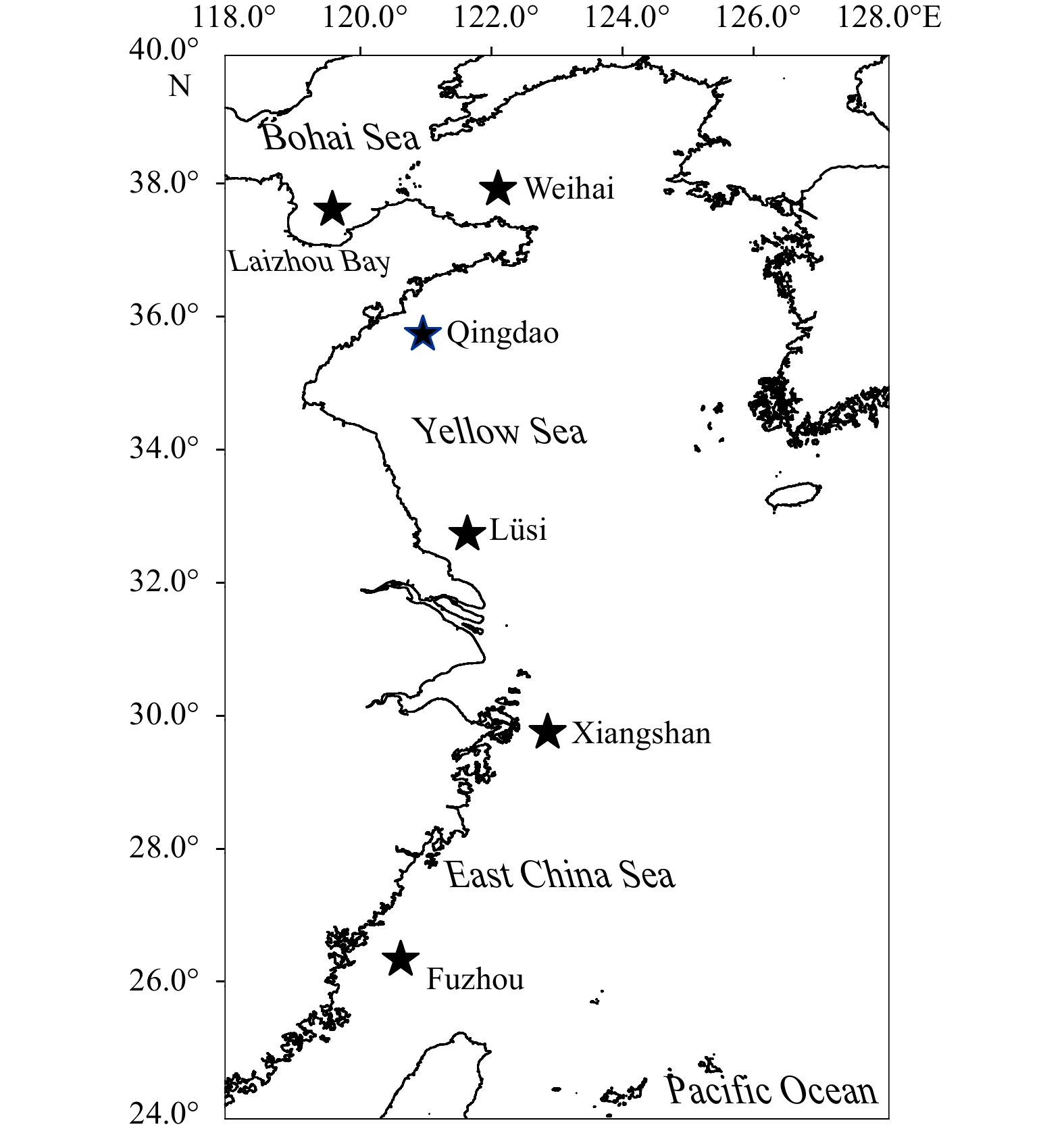
Sampling locations of Japanese Spanish mackerel from six spawning grounds during spring along the eastern coastal waters of China.
| Citation: | Haozhi Sui, Ying Xue, Yunkai Li, Binduo Xu, Chongliang Zhang, Yiping Ren. Feeding ecology of Japanese Spanish mackerel (Scomberomorus niphonius) along the eastern coastal waters of China[J]. Acta Oceanologica Sinica, 2021, 40(8): 98-107. doi: 10.1007/s13131-021-1796-0

|
Coastal ecosystems are continually impacted by climate change and other social stressors, such as rising and warming seas, intensifying storms and droughts, acidifying oceans, and overfishing (Bunce et al., 2010; Chuenpagdee and Jentoft, 2009; Cinner et al., 2012; Perry et al., 2011; Zou and Wei, 2010). Habitat degradation and fishing exploitation have generated a strong impact on marine fauna in recent decades. Fish communities are also threatened by multiple stressors. Most species change their life history strategies to adapt to different stressors by migrating or changing their feeding strategies.
Profound declines in some populations of traditional Chinese fishery species (e.g., Larimichthys crocea, Pampus argenteus, Sepiella maindroni) have become apparent owing to long-term disturbances such as intense fishing exploitation, pollution and habitat degradation. In contrast, Japanese Spanish mackerel (Scomberomorus niphonius) supported major marine commercial fisheries in China with an annual landing of more than 400 000 tonnes (Zhang et al., 2016). It appears that this fish has a unique capacity for adaptation to the changing environment.
Japanese Spanish mackerel is a migratory, coastal pelagic species widely distributed in the northwestern Pacific (Xing et al., 2009). Matured adults of this species spawn in eastern coastal waters from the East China Sea to the Bohai Sea in spring (Qiu and Ye, 1996). It was reported that this species might be composed of three stocks, i.e., the southern stock (in the southern East China Sea), the middle stock (in the middle Yellow Sea) and the northern stock (in the northern Yellow Sea and Bohai Sea) (Wei and Zhou, 1988; Zhang et al., 2016). According to previous studies, Japanese Spanish mackerel demonstrated a strong dietary preference for forage fish, especially for Japanese anchovy (Engraulis japonicus) (Deng et al., 1986; Wu, 1987). Heavy exploitation of Japanese anchovies in the East China Sea and Yellow Sea has raised concerns about possible resource depletion and recruitment failure of Japanese Spanish mackerel. In addition, the biological characteristics of the Japanese Spanish mackerel population have been continuously adjusted to adapt to intensive fishing, which was obviously manifested in accelerated growth rate, early sexual maturity and extended spawning period. The minimum fork length at first sexual maturity decreased from (52.9±0.3) cm (before 1962) to (42.4±0.2) cm (1977–1989) and further to (38.0±2.3) cm (after 1997) (Sun, 2009). Previous studies have focused more on the individual growth characteristics of Japanese Spanish mackerel, such as fork length and body weight, and feeding ecology has not yet been reported. However, changes in the characteristics of the population are multifaceted and interactive. It is necessary to determine whether feeding activities have changed and what kinds of changes have occurred in feeding patterns to maintain the population of Japanese Spanish mackerel. Therefore, it is worth exploring the mechanism underlying the ecological aspects of basic feeding that facilitate their capacity to adapt, particularly in terms of trophic ecology for reproduction.
Feeding strategies are the key to understanding the mechanisms driving the survival, growth, and reproduction of fish species (Stearns, 1992). Feeding activities provide nutrition and energy to support the maintenance, growth, reproduction, and development of fish populations (Liu et al., 2009). Among these, reproduction has been identified as the most metabolically demanding process, during which high amounts of nutrients and energy are required for the production of hormones and gametes, development of secondary sexual characteristics and reproductive physiology of fishes (Zudaire et al., 2015). Reproductive output is important for determining recruitment and population dynamics (Stearns, 1992; McGraw and Caswell, 1996; Li et al., 2007). Therefore, information about the feeding ecology of spawning groups is critical for the assessment and management of commercially important fish species (Liu et al., 2009).
The trophic ecology of fishes has traditionally been examined by stomach content analysis (Hyslop, 1980; Cortés, 1999). This methodology is one of the most widely used methods to provide detailed information on diet composition, prey size, consumption rates and foraging habitats of species (Chipps and Garvey, 2007), although it might be biased by opportunistic feeding and different digestion rates of prey (Tsai et al., 2015). In addition, stable isotope analysis is able to track diets over longer time periods (Reum and Essington, 2013). The δ13C values remain relatively constant between prey and predators but vary between different primary producers and environments (Tieszen et al., 1983; Peterson and Fry, 1987; Boutton, 1991). Therefore, carbon sources can be used to determine the dietary source of a consumer (Munroe et al., 2014). δ15N values can be used to estimate the trophic position of individuals. Tissue isotope values more rapidly reflect a recent diet in the liver (weeks) than in muscle (months) (Logan et al., 2006). Analysis of both tissues can provide more comprehensive dietary information over different timescales, showing the changes in dietary resources, and can be used to estimate residency in sampling regions (Goñi et al., 2011).
The aim of this study was to examine the trophic ecology of Japanese Spanish mackerel spawning groups along the eastern coastal waters of China based on both stomach content analysis and stable isotope analysis. Specifically, the objectives were (1) to investigate the dietary plasticity of Japanese Spanish mackerel over a long-term period by comparison with historical data, (2) to determine the spatial trophic adaptability of Japanese Spanish mackerel spawning groups from six spawning grounds along the eastern coastal waters of China, and (3) to examine the effects of different methods on the feeding ecology of this species. The study could provide essential information about the trophic ecology and dietary plasticity of Japanese Spanish mackerel and help to manage the population of this species.
Samples were collected from six spawning grounds of Japanese Spanish mackerel along the eastern coastal waters of China (25.00°–38.00°N, 118.00°–124.00°E) by commercial fisheries (using gillnets) during spring (March to May) in 2016 and 2017 (Fig. 1). Samples were kept on ice for several hours onboard and then frozen (−20°C) in the laboratory. Each individual was weighed to the nearest gram, and the fork length was measured to the nearest millimetre. Total length, weight, gonad weight and liver weight were also measured (China National Standardization Management Committee, 2007). Samples of liver tissue (approximately 5 g) and dorsal muscle (below the first dorsal fin of fish; approximately 5 g) were collected and stored at −20°C for stable isotope analysis.
A total of 590 stomachs of Japanese Spanish mackerel were analysed (Table 1). Samples were cleaned thoroughly in distilled water before dissection. Stomach and foreguts of Japanese Spanish mackerel were separated and placed on slides, and all food contents were scraped or squeezed out under a dissecting microscope. Gut contents were then dispersed gently using a dissecting needle with care to avoid damaging food items (China National Standardization Management Committee, 2007). Each prey item was identified as the lowest taxonomic unit. Three indices were calculated, i.e., weight percentage (W%), number percentage (N%), and frequency of occurrence (F%). The index of relative importance (IRI) and percentage IRI (IRI%) were also calculated (Cortés, 1997; Jacob et al., 2005):
| Locations | n | Empty-stomach rate | Fork length/cm | Sex | Number for isotopic analysis | ||||||
| mean | SD | range | ♀ | ♂ | muscle | liver | |||||
| Fuzhou | 83 | 20.48% | 48.26 | ±4.74 | 41.5–63.4 | 59 | 23 | 4 | 3 | ||
| Xiangshan | 112 | 67.86% | 59.65 | ±7.99 | 44.2–102.5 | 10 | 85 | 15 | 6 | ||
| Lüsi | 153 | 36.60% | 48.94 | ±6.94 | 40.5–89.5 | 54 | 99 | 11 | 5 | ||
| Qingdao | 151 | 19.21% | 54.15 | ±10.92 | 40.8–90.8 | 51 | 100 | 19 | 7 | ||
| Weihai | 44 | 15.91% | 54.17 | ±14.61 | 35.3–89.6 | 10 | 33 | 8 | 5 | ||
| Laizhou Bay | 47 | 68.09% | 81.50 | ±6.68 | 70.2–101.0 | 41 | 6 | 5 | 4 | ||
| Total | 590 | 36.78% | 55.20 | ±12.38 | 35.3–102.5 | 225 | 346 | 62 | 30 | ||
 DownLoad:
CSV
DownLoad:
CSV
| $$ {\rm{IRI}}=\left(W\%+N\%\right)\times F\%{\rm{,}} $$ | (1) |
| $$ {\rm{IRI}}\%=\left[{\rm{IRI}}/\sum \left({\rm{IRI}}\right)\right]\times 100. $$ | (2) |
To examine the ontogenetic variations in the feeding ecology of Japanese Spanish mackerel, individuals were divided into seven fork length classes by 10 cm, i.e., 40–49 cm, 50–59 cm, 60–69 cm, 70–79 cm, 80–89 cm, 90–99 cm and 100–109 cm.
A total of 62 samples of white muscle (approximately 5 g) and 30 samples of liver tissue of Japanese Spanish mackerel were collected for stable isotope analysis (Table 1). All 92 samples met three selection criteria: (1) samples were intact; (2) samples covered the range of fork length for each location; and (3) the number of samples was sufficient for statistical analysis (n≥3). Tissue samples must be acidified to make stable isotope data comparable across taxa with varying CaCO3 contents (Jacob et al., 2005). Dissected tissues were acidified (3% HCl) to remove residual carbonates, rinsed with distilled water, dried at 60°C for approximately 24 h, and ground into powder. Muscle tissues of potential prey items in sampling locations were treated in the same way.
Stable isotope ratios were expressed in δ notation as deviations from standards in parts per thousand (‰) using the following equation:
| $$ \delta X=\left[\left({R}_{\mathrm{s}\mathrm{a}\mathrm{m}\mathrm{p}\mathrm{l}\mathrm{e}}/{R}_{\mathrm{s}\mathrm{t}\mathrm{a}\mathrm{n}\mathrm{d}\mathrm{a}\mathrm{r}\mathrm{d}}\right)-1\right]\times 1\;000{\rm{,}} $$ | (3) |
where X is 13C or 15N, Rsample is the ratio (13C/12C or 15N/14N) in samples, and Rstandard is the ratio in the standard. The standard reference for carbon was Pee Dee Belemnite carbonate, and nitrogen was atmospheric N2 (Reum and Essington, 2013).
Trophic levels (TL) of Japanese Spanish mackerel and their potential prey items were calculated by the following equation:
| $$ {\rm{TL}}=\left[\frac{\delta {}^{15}{{\rm{N}}}_{\mathrm{s}\mathrm{a}\mathrm{m}\mathrm{p}\mathrm{l}\mathrm{e}}-\delta {}^{15}{{\rm{N}}}_{\mathrm{b}\mathrm{a}\mathrm{s}\mathrm{e}\mathrm{l}\mathrm{i}\mathrm{n}\mathrm{e}}}{{\rm{TEF}}}\right]+{{\rm{TL}}}_{\mathrm{b}\mathrm{a}\mathrm{s}\mathrm{e}\mathrm{l}\mathrm{i}\mathrm{n}\mathrm{e}}{\rm{,}} $$ | (4) |
where δ15Nbaseline and TLbaseline are the known median δ15N value (4.90‰) and trophic level of trophic baseline species (small copepods in this study), respectively (Post, 2002). The trophic enrichment factor (TEF) represents the best estimate of isotopic enrichment between prey and predators. An TEF of 3.4‰ was adopted in this study based on the literature that reported consumer-diet δ15N enrichment (Caut et al., 2009).
δ15N and δ13C values of Japanese Spanish mackerel were used to calculate the isotopic niche based on muscle and liver tissue. The isotopic niche was calculated using the SIBER of the SIAR package (Parnell et al., 2010) in RStudio version 1.0.136 as described by Jackson (Jackson et al., 2011). This method uses Bayesian inference techniques to produce (1) the smallest convex hulls that contain all individual δ15N and δ13C values within a sample area to represent the total niche breadth area and (2) Bayesian standard ellipses (SEAb) that incorporate the 90% densest data points within a dataset and thus better represent the “average” isotopic niche breadth of the population (Jackson et al., 2011; Layman et al., 2007; Suca and Llopiz, 2017). This method was chosen because a Bayesian framework for isotopic niche calculations better accounts for sources of uncertainty and variability inherent in stable isotope analysis and allows for more robust comparisons between groups, particularly for small and/or variable sample sizes (Parnell et al., 2010). The relative contributions of all potential prey items to the diet composition of Japanese Spanish mackerel were calculated by a two-source Bayesian mixing model with the SIAR package in RStudio version 1.0.136.
The gonad development stage of all samples of Japanese Spanish mackerel was checked, including all stages I to VI (Table 2). The fork length of samples of Japanese Spanish mackerel ranged from 35.3 cm to 102.5 cm. The minimum 35.3 cm came from a female at gonad development stage IV. The fork lengths of the other samples were all greater than the minimum (35.7 cm) indicated by previous research above, belonging to the mature population. Eighty percent of Japanese Spanish mackerel samples were mature (stage IV–VI).
| Gonad development stage | n | Fork length/cm | Body weight/g | |||||
| mean | SD | range | mean | SD | range | |||
| I | 21 | 61.6 | 11.3 | 38.8–86.8 | 806 | 274 | 453–1 067 | |
| II | 59 | 45.5 | 2.3 | 41.5–52.5 | 783 | 134 | 575–1 257 | |
| III | 38 | 55.3 | 7.8 | 42.3–74.0 | 1 309 | 466 | 629–2 820 | |
| IV | 71 | 51.1 | 9.4 | 35.3–89.5 | 1 172 | 875 | 371–6 537 | |
| V | 302 | 58.8 | 14.5 | 40.5–102.5 | 1 886 | 1543 | 539–10 936 | |
| VI | 99 | 51.7 | 5.5 | 40.6–70.4 | 1 078 | 318 | 533–2 408 | |
DownLoad:
CSV
Among the 590 stomachs of Japanese Spanish mackerel, 63.22% (n=373) contained food in their stomachs, and 36.78% (n=217) were empty. The empty stomach rates in Xiangshan and Laizhou Bay were much higher than those in the other four locations (67.86% and 68.09%, respectively). A total of 41 prey items were identified, comprising 24 teleost fish species and 17 invertebrate species. Prey items could mainly be classified into three groups, i.e., fish, crustaceans and cephalopods (Table 3). The most important prey groups were fish. According to IRI%, the dominant prey species were the fish Japanese anchovy and sand lance (Ammodytes personatus) and the shrimp Leptochela gracilis.
| Prey items | Fuzhou | Xiangshan | Lüsi | Qingdao | Weihai | Laizhou Bay | Total |
| Pisces | |||||||
| Engraulis japonicus | 1.01 | 33.55 | 21.69 | 0.36 | 0.97 | 23.54 | 6.44 |
| Ammodytes personatus | 80.97 | 91.18 | 13.22 | 54.18 | |||
| Enedrias fangi | 0.67 | 0.09 | 0.05 | 0.30 | |||
| Benthosema pterotum | 0.03 | 0.09 | 0.01 | ||||
| Larimichthys polyactis | 0.47 | 0.03 | 0.01 | ||||
| Liza haematocheila | 0.10 | 0.03 | |||||
| Harpadon nehereus | 0.10 | – | |||||
| Champsodon capensis | 0.78 | 0.11 | 0.10 | ||||
| Gonorynchus abbreviatus | 0.02 | – | |||||
| Thryssa mystax | 1.29 | 0.09 | |||||
| Thryssa kammalensis | 4.40 | 4.08 | 0.89 | ||||
| Callionymus richardsoni | – | – | |||||
| Coilia mystus | 2.20 | 0.01 | 0.14 | ||||
| Bregmaceros pescadorus | 0.17 | 0.03 | 0.02 | ||||
| Synodus macrops | 0.04 | – | |||||
| Decapterus maruadsi | 0.01 | – | |||||
| Hyporhamphus sajori | 2.23 | 0.08 | |||||
| Liparis | 0.56 | 0.02 | |||||
| Thryssa | 0.23 | 0.47 | 0.02 | ||||
| Stolephorus | 81.52 | 5.08 | |||||
| Sardinella | 0.19 | 0.05 | 0.07 | ||||
| Trichiurus | 0.01 | – | |||||
| Engraulidae | 11.45 | 0.03 | |||||
| Gobiinae | 0.19 | 0.01 | 0.02 | ||||
| unidentified pisces | 2.83 | 47.21 | 1.27 | 0.04 | 0.10 | 1.30 | |
| Crustacea | |||||||
| Euphausiacea | |||||||
| Euphausia pacifica | 48.87 | 3.00 | |||||
| Decapoda | |||||||
| Latreutes planircstris | – | 0.14 | 0.01 | ||||
| Leptochela gracilis | 5.22 | 0.06 | 15.65 | 5.78 | 61.11 | 25.17 | |
| Crangon affinis | 0.01 | – | |||||
| Acetes chinensis | 20.36 | 1.24 | |||||
| unidentified decapoda | 0.01 | 0.16 | – | 0.02 | 0.03 | ||
| Stomatopoda | |||||||
| Oratosquilla oratoria | – | – | |||||
| Mysidacea | |||||||
| Neomysis japonica | 0.01 | 0.03 | 0.01 | ||||
| Amphipoda | |||||||
| Parathemisto gracilipes | 1.14 | 0.62 | 0.34 | 2.07 | 0.73 | ||
| Gammarus sp. | 0.09 | 0.03 | – | 0.15 | 0.02 | ||
| Copepoda | |||||||
| Calanidae | 5.51 | 1.46 | 1.15 | 0.92 | |||
| Brachyura | |||||||
| Charybdis bimaculata | 0.01 | – | |||||
| Cephalopoda | |||||||
| Loligo sp. | 0.04 | 0.01 | 0.01 | ||||
| Euprymna morsei | – | – | |||||
| Sepiola birostrata | 0.04 | – | |||||
| Sepiolidae | 0.03 | – | – | ||||
| Sepiida | 0.03 | – | – | ||||
| Unidentified cephalopoda | 0.07 | 0.01 | 0.01 | ||||
| Gastropoda | |||||||
| Philine kinglipini | 0.01 | – | |||||
| Algae | 0.04 | 0.05 | 0.01 | ||||
| Unidentified items | 0.02 | 0.01 | |||||
| Note: the dash “–” indicates that a value <0.01, but not a missing value. | |||||||
DownLoad:
CSV
The dominant food of Japanese Spanish mackerel was significantly different among sampling locations (Table 3). The most important prey species were Stolephorus (IRI%=81.52%) in Fuzhou, Japanese anchovy (33.55%) in Xiangshan, E. pacifica (48.87%) in Lüsi, sand lance (80.97%, 91.18%) in Qingdao and Weihai, and L. gracilis (61.11%) in Laizhou Bay. The contribution of other prey items also showed great spatial variations.
There were no significant differences in the stable isotopic values of muscle tissue (p>0.05) and liver tissue (p>0.05) between males and females, so samples of males and females were pooled for further analyses. The δ15N values of Japanese Spanish mackerel ranged from 10.50‰ to 15.50‰ (12.97‰±1.00‰) for muscles and 8.61‰ to 14.20‰ (11.47‰±1.10‰) for livers. The δ13C values of Japanese Spanish mackerel ranged from −19.96‰ to −16.38‰ (−18.45‰±0.84‰) for muscles and −22.37‰ to −19.38‰ (−20.76‰±0.75‰) for livers.
The samples were divided into seven size classes of fork length (Fig. 2). The mean δ15N and δ13C values in livers were typically lower than the mean δ15N and δ13C values in muscles for each fork length class (Fig. 2). The mean δ15N values of muscles increased from 30–39 cm to 70–79 cm but decreased from 70–79 cm to 90–99 cm. The mean δ15N values of the livers increased from 30–39 cm to 60–69 cm but showed a slight decrease from 60–69 cm to 90–99 cm. There was no significant relationship between the mean δ13C values and fork length for either muscle or liver (p>0.05).

δ15N and δ13C for Japanese Spanish mackerel and their potential prey items are shown in Fig. 3. Both δ15N and δ13C values showed large differences across a wide range of prey items (Fig. 3). Potential prey items of Japanese Spanish mackerel were aggregated into nine groups, i.e., Japanese anchovy, sand lance, Thryssa kammalensis, other pelagic fishes (Konosirus punctatus, Setipinna tenuifilis, Sardinella zunasi), other demersal fishes (Enedrias fangi, Callionymus richardsoni, Amblychaeturichthys hexanema, Chaeturichthys stigmatias, Ctenogobius pflaumi, Pseudosciaena polyactis), L. gracilis, E. pacifica, other crustaceans (Metapenaeopsis dalei, Crangon affinis, Trachysalambria curvirostris, Latreutes planirostris), and cephalopods (Euprymna morsei, Loligo spp.). Mean δ15N values of potential prey items ranged from 6.30‰ (E. pacifica) to 12.37‰ (cephalopod) (Δ6.07‰), and δ13C values ranged from −21.99‰ (sand lance) to −18.00‰ (other demersal fishes) (Δ3.99‰). The dots with different shapes represent different size classes of Japanese Spanish mackerel individuals. Dots mixed together and could not be separated clearly (Fig. 3). This shows that there was no obvious ontogenetic feeding change between different size classes of Japanese Spanish mackerel.

Trophic levels of Japanese Spanish mackerel showed a positive trend with fork length (Fig. 4). Japanese Spanish mackerel displayed a wide range of trophic levels, shifting from 4.08±0.42 (30–39 cm) to 4.48±0.01 (70–79 cm).

The cluster analysis showed the interrelation of diet compositions of Japanese Spanish mackerel in six sampling locations (Fig. 5). The dendrograms displayed similar structures of diet compositions with a convincingly higher value among Qingdao, Weihai and Laizhou Bay. In turn, there was the lowest value of similarity of Xiangshan with the other locations (Fig. 5).

The stable isotope values of Japanese Spanish mackerel showed spatial variations (Table 4). The mean δ15N values in muscles in Fuzhou and Xiangshan were lower than those in other locations. The δ13C values in muscle and liver showed little difference among locations, suggesting a consistent variation in all sampling locations.
| Locations | Muscle | Liver | |||||
| δ15N/‰ | δ13C/‰ | TL | δ15N/‰ | δ13C/‰ | TL | ||
| Fuzhou | 12.39±1.09 | −18.23±1.00 | 4.20±0.32 | 12.10±0.73 | −20.34±0.79 | 4.12±0.22 | |
| Xiangshan | 12.47±0.69 | −17.52±0.80 | 4.24±0.21 | 11.98±1.30 | −19.79±0.24 | 4.08±0.38 | |
| Lüsi | 13.34±1.08 | −18.79±0.63 | 4.42±0.25 | 11.47±0.39 | −20.92±0.40 | 3.93±0.11 | |
| Qingdao | 13.15±0.81 | −18.80±0.56 | 4.43±0.24 | 11.33±0.66 | −21.41±0.69 | 3.89±0.19 | |
| Weihai | 13.52±0.78 | −18.66±0.71 | 4.54±0.23 | 11.65±0.59 | −21.15±0.79 | 3.99±0.17 | |
| Laizhou Bay | 13.63±0.59 | −18.43±0.87 | 4.57±0.17 | 11.69±0.48 | −20.54±0.74 | 4.00±0.14 | |
DownLoad:
CSV
In addition, the δ15N and δ13C values in muscles were higher than those in livers in all sampling locations. Japanese Spanish mackerel exhibited a larger range of δ15N values in muscles ranging from 12.39‰ to 13.63‰ (mean ± SD, 13.07‰±0.90‰), with a smaller range in livers from 11.33‰ to 12.10‰ (11.63‰±0.71‰). The δ15N values in muscles increased with latitude, while livers changed little with latitude.
The trophic levels of Japanese Spanish mackerel from six sampling locations were significantly different (p<0.05) (Table 4). The trophic levels ranged from 4.20±0.32 to 4.57±0.17 (Δ 0.35) in muscle, increasing with latitude from the south (Fuzhou) to the north (Laizhou Bay).
The isotope biplot for Japanese Spanish mackerel is shown in Fig. 6. The isotopic niche of Japanese Spanish mackerel moderately overlapped among six locations, but the degree of overlap varied spatially, with the overlap being the smallest between Xiangshan and Lüsi (0 for muscle and liver) and the largest between Lüsi and Weihai (74.16% and 55.30% for muscle and liver) (Fig. 6). The isotope niche sizes of Japanese Spanish mackerel in Fuzhou and Xiangshan were larger than those in the other four locations.

Stomach content analysis produced similar results as previous studies, showing that Japanese Spanish mackerel mainly fed on fish (W%=92.21%). During the 1980s, Japanese anchovy was the most important prey item (W%>98%) for Japanese Spanish mackerel (Wu, 1987). In this study, Japanese anchovy was still an important prey item for Japanese Spanish mackerel in Xiangshan, Lüsi and Laizhou Bay (W%=67.18%, 25.44%, 42.93%, respectively) but accounted for less than 10% in other locations. The decreased proportion of Japanese anchovies in the diet was mainly due to the sharp decline in its population in Chinese seas caused by overfishing (Zhao et al., 2010; Jin et al., 2005). In this case, Japanese Spanish mackerel showed high dietary adaptability, with its major prey species switching from Japanese anchovy to other prey species, which is probably one of the main reasons that the Japanese Spanish mackerel has survived intense fishing exploitation and other stressors.
Sand lance, a small pelagic fish species, has become the most important prey item for the northern stock of Japanese Spanish mackerel, with weight percentages of 80.77% and 92.23% in Qingdao and Weihai, respectively. Sand lance is a key species in the China seas. Replacing the declining anchovy population, the biomass of sand lance increased and became the dominant prey fish in the Bohai Sea and Yellow Sea (Li, 2015; Wo et al., 2018). It displays a seasonal energy cycle with a 31% increase in energy density (kJ/g) between February and June (Robards et al., 1999). The lipid content of other prey species also increases rapidly prior to summer (e.g., sand lance and Ammodytes marinus) (Sekiguchi, 1977; Hislop et al., 1991). Sand lance may provide enough energy to its predators, including Japanese Spanish mackerel, and become the preferred prey. Japanese Spanish mackerel showed an adaptive feeding strategy and switched its main prey item from anchovy to sand lance and other available prey according to the abundance of these forage species. This dietary plasticity will be beneficial to the maintenance, growth, reproduction and survival of Japanese Spanish mackerel.
The empty stomach rates in Xiangshan and Laizhou Bay were much higher than those in the other four locations. This observation might lead to the assumption that Japanese Spanish mackerel does not ingest significantly until arriving at its final spawning grounds, and its feeding behaviour mainly occurs during prespawning migration. It is known that food deprivation may cause increased δ15N values and decreased somatic conditions (Gannes et al., 1997; Hobson et al., 1993). However, there was no significant increase in δ15N values in Xiangshan and Laizhou Bay, suggesting that either foraging occurs or stored nutriment reserves can cope with the energy costs associated with reproductive migration.
This study showed that there were obvious spatial variations in the trophic ecology of Japanese Spanish mackerel among six spawning grounds along the coastal China seas. In the southern East China Sea, mackerels mainly consume Stolephorus sp. In the northern East China Sea, mackerels mainly consume Japanese anchovies and E. pacifica. In the Yellow Sea and Bohai Sea, mackerels mainly consume sand lance, Japanese anchovy and L. gracilis. These differences provided phenotypic evidence for the stock identification and migration trajectories of Japanese Spanish mackerel. The three geographic stocks experienced different environments associated with migration trajectories based on analysis of their otolith features (Zhang et al., 2016). The feeding preference of Japanese Spanish mackerel and the availability of local prey species in each spawning ground were the main reasons for the spatial difference in the trophic ecology of Japanese Spanish mackerel.
The δ15N value has proven effective in elucidating size-related changes in the trophic level of many fish species (Lindsay et al., 1998; Overman and Parrish, 2001; Jennings et al., 2002). δ15N enrichment across different size classes of fishes demonstrated that trophic positions within a community were largely determined by the size of organisms (Jennings et al., 2002). Thus, the differences in δ15N values between sampling locations probably represent differences in the size or trophic positions of prey items consumed. The overall increase in trophic positions with size is generally considered to be the result of intraspecific accumulation of heavy isotopes with somatic growth in body mass (Lindsay et al., 1998; Jennings et al., 2002). For Japanese Spanish mackerel, the δ15N values in muscle increased with latitude from south to north along the coastal China seas, and the trophic levels showed a consistent trend with δ15N values. These trends are anastomotic with the migration route of Japanese Spanish mackerel from south to north during the spawning period. It has been proven that the gape size of Japanese Spanish mackerel is significantly correlated with its body length (Lin et al., 2017). When migrating from south to north, it probably consumed larger prey to accumulate more energy for growth.
Prey items in the diet and niche breadth could considerably influence the geographic variation in trophic ecology (Munroe et al., 2014). For Japanese Spanish mackerel, the isotopic niche breadth differed greatly among different locations. The highly overlapping isotopic niches of four spawning grounds (Lüsi, Qingdao, Weihai and Laizhou Bay) suggested a higher level of food competition in their local ecosystems. Moreover, the wider trophic niche of stock in Fuzhou indicated higher variability in individual diets. These differences might be due to geographic variations in local prey items. The lower specialized diets of Japanese Spanish mackerel might result in a larger isotopic niche or larger niche overlap compared with other spawning grounds. The results support the hypothesis that changes in fish growth, size and ultimately accumulation could be due to bottom-up control characterized by changes in food availability and increasing potential trophic competition.
When prior information on diet composition is limited because of the high empty stomach rate, employing representative prey items in isotope mixing models can provide useful information on diets (Polito et al., 2011). For the parameterization of the multisource SIAR model, pertinent prey items were identified mainly from the analysis of hard remains from the stomach contents and previous studies carried out in the same waters. The results of stomach content analysis and stable isotope analysis could be combined to obtain an accurate diet composition of fishes.
Stable isotope values in the liver and muscle of Japanese Spanish mackerel showed some differences. In general, δ15N values increase from prey to predators and accumulate persistently in individuals (Peterson and Fry, 1987; Minagawa and Wada, 1984). In this study, there was a positive correlation between fish fork length and δ15N values in muscles. Japanese Spanish mackerel consumed more high-trophic-level prey items with increasing size. However, the stable isotope values in the liver did not show the same result as those in muscle. Japanese Spanish mackerel with 60–69 cm fork length had the highest δ15N values in the liver, while mackerel with 70–79 cm fork length had the highest δ15N values in muscle. This could be explained by the fact that livers had higher isotopic turnover rates and showed foraging habits over shorter time periods than muscle. It is necessary to consider the difference in stable isotope values in different tissues when using stable isotope analysis.
Although stable isotope analysis provides an alternative method to assess trophic relationships and consumption patterns, it is necessary to exercise caution in their interpretation (Brush et al., 2012). It is suggested to combine stomach content analysis and stable isotope analysis from different tissues to obtain more comprehensive information about the feeding ecology of marine species.
We are grateful to many colleagues and students for their assistance in field sampling and sample analyses.
| [1] |
Boutton T W. 1991. Stable carbon isotope ratios of natural materials: II. atmospheric, terrestrial, marine, and freshwater environments. In: Coleman D C, Fry B, eds. Carbon Isotope Techniques. Amsterdam, the Netherlands: Elsevier, 173–185
|
| [2] |
Brush J M, Fisk A T, Hussey N E, et al. 2012. Spatial and seasonal variability in the diet of round goby (Neogobius melanostomus): stable isotopes indicate that stomach contents overestimate the importance of dreissenids. Canadian Journal of Fisheries and Aquatic Sciences, 69(3): 573–586. doi: 10.1139/f2012-001
|
| [3] |
Bunce M, Rosendo S, Brown K. 2010. Perceptions of climate change, multiple stressors and livelihoods on marginal African coasts. Environment, Development and Sustainability, 12(3): 407–440. doi: 10.1007/s10668-009-9203-6
|
| [4] |
Caut S, Angulo E, Courchamp F. 2009. Variation in discrimination factors (Δ15N and Δ13C): the effect of diet isotopic values and applications for diet reconstruction. Journal of Applied Ecology, 46(2): 443–453. doi: 10.1111/j.1365-2664.2009.01620.x
|
| [5] |
China National Standardization Management Committee. 2007. Specifications for oceanographic survey–Part 6: Marine biological survey: GB/T 12763.6-2007 (in Chinese). Beijing: Standards Press of China
|
| [6] |
Chipps S R, Garvey J E. 2007. Assessment of food habits and feeding patterns. In: Guy C, Brown M, eds. Analysis and Interpretation of Freshwater Fisheries Data. Bethesda, MD, USA: American Fisheries Society, 473–514
|
| [7] |
Chuenpagdee R, Jentoft S. 2009. Governability assessment for fisheries and coastal systems: a reality check. Human Ecology, 37(1): 109–120. doi: 10.1007/s10745-008-9212-3
|
| [8] |
Cinner J E, McClanahan T R, Graham N A J, et al. 2012. Vulnerability of coastal communities to key impacts of climate change on coral reef fisheries. Global Environmental Change, 22(1): 12–20. doi: 10.1016/j.gloenvcha.2011.09.018
|
| [9] |
Cortés E. 1997. A critical review of methods of studying fish feeding based on analysis of stomach contents: application to elasmobranch fishes. Canadian Journal of Fisheries and Aquatic Sciences, 54(3): 726–738. doi: 10.1139/f96-316
|
| [10] |
Cortés E. 1999. Standardized diet compositions and trophic levels of sharks. ICES Journal of Marine Science, 56(5): 707–717. doi: 10.1006/jmsc.1999.0489
|
| [11] |
Deng Jingyao, Meng Tianxiang, Ren Shengmin. 1986. Food web of fishes in Bohai Sea. Acta Ecologica Sinica (in Chinese), 6(4): 356–364
|
| [12] |
Gannes L Z, O'Brien D M, del Rio C M. 1997. Stable isotopes in animal ecology: assumptions, caveats, and a call for more laboratory experiments. Ecology, 78(4): 1271–1276. doi: 10.1890/0012-9658(1997)078[1271:SIIAEA]2.0.CO;2
|
| [13] |
Goñi N, Logan J, Arrizabalaga H, et al. 2011. Variability of albacore (Thunnus alalunga) diet in the Northeast Atlantic and Mediterranean Sea. Marine Biology, 158(5): 1057–1073. doi: 10.1007/s00227-011-1630-x
|
| [14] |
Hislop J R G, Harris M P, Smith J G M. 1991. Variation in the calorific value and total energy content of the lesser sandeel (Ammodytes marinus) and other fish preyed on by seabirds. Journal of Zoology, 224(3): 501–517. doi: 10.1111/j.1469-7998.1991.tb06039.x
|
| [15] |
Hobson K A, Alisauskas R T, Clark R G. 1993. Stable-nitrogen isotope enrichment in avian tissues due to fasting and nutritional stress: implications for isotopic analyses of diet. The Condor, 95(2): 388–394. doi: 10.2307/1369361
|
| [16] |
Hyslop E J. 1980. Stomach contents analysis—a review of methods and their application. Journal of Fish Biology, 17(4): 411–429. doi: 10.1111/j.1095-8649.1980.tb02775.x
|
| [17] |
Jackson A L, Inger R, Parnell A C, et al. 2011. Comparing isotopic niche widths among and within communities: SIBER–Stable Isotope Bayesian Ellipses in R. Journal of Animal Ecology, 80(3): 595–602. doi: 10.1111/j.1365-2656.2011.01806.x
|
| [18] |
Jacob U, Mintenbeck K, Brey T, et al. 2005. Stable isotope food web studies: a case for standardized sample treatment. Marine Ecology Progress Series, 287: 251–253. doi: 10.3354/meps287251
|
| [19] |
Jennings S, Warr K J, Mackinson S. 2002. Use of size-based production and stable isotope analyses to predict trophic transfer efficiencies and predator-prey body mass ratios in food webs. Marine Ecology Progress Series, 240: 11–20. doi: 10.3354/meps240011
|
| [20] |
Jin Xianshi, Zhao Xianyong, Meng Tianxiang, et al. 2005. Biological Resources and Habitat in the Yellow Sea and Bohai Sea (in Chinese). Beijing: Science Press
|
| [21] |
Layman C A, Arrington D A, Montaña C G, et al. 2007. Can stable isotope ratios provide for community-wide measures of trophic structure?. Ecology, 88(1): 42–48. doi: 10.1890/0012-9658(2007)88[42:CSIRPF]2.0.CO;2
|
| [22] |
Li Chao. 2015. Selectivity of codend mesh of double stake and two-stick stow net in the coast of the Zhaitang Island, Qingdao (in Chinese)[dissertation]. Qingdao: Ocean University of China
|
| [23] |
Li Yuxuan, Xie Songguang, Li Zhongjie, et al. 2007. Gonad development of an anadromous fish Coilia ectenes (Engraulidae) in lower reach of Yangtze River, China. Fisheries Science, 73(6): 1224–1230
|
| [24] |
Lin Nan, Wang Yutan, Chen Yuange, et al. 2017. Feeding habits of Japanese Spanish mackerel (Scomberomorus niphonius) larvae and juveniles in Xiangshan Bay. Chinese Journal of Ecology (in Chinese), 36(10): 2811–2816
|
| [25] |
Lindsay D J, Minagawa M, Mitani I, et al. 1998. Trophic shift in the Japanese anchovy Engraulis japonicus in its early life history stages as detected by stable isotope ratios in Sagami Bay, Central Japan. Fisheries Science, 64(3): 403–410. doi: 10.2331/fishsci.64.403
|
| [26] |
Liu Yong, Cheng Jiahua, Chen Yong. 2009. A spatial analysis of trophic composition: a case study of hairtail (Trichiurus japonicus) in the East China Sea. Hydrobiologia, 632(1): 79–90. doi: 10.1007/s10750-009-9829-2
|
| [27] |
Logan J, Haas H, Deegan L, et al. 2006. Turnover rates of nitrogen stable isotopes in the salt marsh mummichog, Fundulus heteroclitus, following a laboratory diet switch. Oecologia, 147(3): 391–395. doi: 10.1007/s00442-005-0277-z
|
| [28] |
McGraw J B, Caswell H. 1996. Estimation of individual fitness from life-history data. The American Naturalist, 147(1): 47–64. doi: 10.1086/285839
|
| [29] |
Minagawa M, Wada E. 1984. Stepwise enrichment of 15N along food chains: further evidence and the relation between δ15N and animal age. Geochimica et Cosmochimica Acta, 48(5): 1135–1140. doi: 10.1016/0016-7037(84)90204-7
|
| [30] |
Munroe S E M, Heupel M R, Fisk A T, et al. 2014. Geographic and temporal variation in the trophic ecology of a small-bodied shark: evidence of resilience to environmental change. Canadian Journal of Fisheries and Aquatic Sciences, 72(3): 343–351
|
| [31] |
Overman N C, Parrish D L. 2001. Stable isotope composition of walleye: 15N accumulation with age and area-specific differences in δ13C. Canadian Journal of Fisheries and Aquatic Sciences, 58(6): 1253–1260. doi: 10.1139/f01-072
|
| [32] |
Parnell A C, Inger R, Bearhop S, et al. 2010. Source partitioning using stable isotopes: coping with too much variation. PLoS ONE, 5(3): e9672. doi: 10.1371/journal.pone.0009672
|
| [33] |
Perry R I, Ommer R E, Barange M, et al. 2011. Marine social–ecological responses to environmental change and the impacts of globalization. Fish and Fisheries, 12(4): 427–450. doi: 10.1111/j.1467-2979.2010.00402.x
|
| [34] |
Peterson B J, Fry B. 1987. Stable isotopes in ecosystem studies. Annual Review of Ecology and Systematics, 18: 293–320. doi: 10.1146/annurev.es.18.110187.001453
|
| [35] |
Polito M J, Trivelpiece W Z, Karnovsky N J, et al. 2011. Integrating stomach content and stable isotope analyses to quantify the diets of pygoscelid penguins. PLoS ONE, 6(10): e26642. doi: 10.1371/journal.pone.0026642
|
| [36] |
Post D M. 2002. Using stable isotopes to estimate trophic position: models, methods, and assumptions. Ecology, 83(3): 703–718. doi: 10.1890/0012-9658(2002)083[0703:USITET]2.0.CO;2
|
| [37] |
Qiu Shengyao, Ye Maozhong. 1996. Studies on the reproductive biology of Scomberomorus niphonius in the Yellow Sea and Bohai Sea. Oceanologia et Limnologia Sinica (in Chinese), 27(5): 463–470
|
| [38] |
Reum J C P, Essington T E. 2013. Spatial and seasonal variation in δ15N and δ13C values in a mesopredator shark, Squalus suckleyi, revealed through multitissue analyses. Marine Biology, 160(2): 399–411. doi: 10.1007/s00227-012-2096-1
|
| [39] |
Robards M D, Anthony J A, Rose G A, et al. 1999. Changes in proximate composition and somatic energy content for Pacific sand lance (Ammodytes hexapterus) from Kachemak Bay, Alaska relative to maturity and season. Journal of Experimental Marine Biology and Ecology, 242(2): 245–258. doi: 10.1016/S0022-0981(99)00102-1
|
| [40] |
Sekiguchi H. 1977. On fat deposits of the spawners of sand-eels in ise bay, central Japan. Bulletin of the Japanese Society of Scientific Fisheries (in Japanese), 43(2): 123–127. doi: 10.2331/suisan.43.123
|
| [41] |
Stearns S C. 1992. The Evolution of Life Histories. Oxford, UK: Oxford University Press
|
| [42] |
Suca J J, Llopiz J K. 2017. Trophic ecology of barrelfish (Hyperoglyphe perciformis) in oceanic waters of southeast Florida. Bulletin of Marine Science, 93(4): 987–996. doi: 10.5343/bms.2017.1003
|
| [43] |
Sun Benxiao. 2009. The current situation and conservation of Scomberomorus niphonius in Yellow Sea and Bohai Bay (in Chinese)[dissertation]. Beijing: Graduate School of Chinese Academy of Agricultural Sciences
|
| [44] |
Tieszen L L, Boutton T W, Tesdahl K G, et al. 1983. Fractionation and turnover of stable carbon isotopes in animal tissues: implications for δ13C analysis of diet. Oecologia, 57(1–2): 32–37. doi: 10.1007/BF00379558
|
| [45] |
Tsai C N, Chiang W C, Sun Chilu, et al. 2015. Stomach content and stable isotope analysis of sailfish (Istiophorus platypterus) diet in eastern Taiwan waters. Fisheries Research, 166: 39–46. doi: 10.1016/j.fishres.2014.10.021
|
| [46] |
Wei Cheng, Zhou Binbin. 1988. The identifications of populations of the Spanish mackerel, Scomberomorus mphonius (Cuvier et Valenciennes) in the Bohai Sea and the Yellow Sea. Acta Zoologica Sinica (in Chinese), 34(1): 71–81
|
| [47] |
Wo Jia, Mou Xiuxia, Xu Binduo, et al. 2018. Interannual changes in fish community structure in the northern part of the coastal waters of Jiangsu Province, China in spring. Chinese Journal of Applied Ecology (in Chinese), 29(1): 285–292
|
| [48] |
Wu Wenkui. 1987. Oral appendage structure and feeding habit of Spanish mackerel in Qingdao coastal waters in spring fishing season. Acta Oceanologica Sinica, 12(4): 643–647
|
| [49] |
Xing Shichao, Xu Genbo, Liao Xiaolin, et al. 2009. Twelve polymorphic microsatellite loci from a dinucleotide-enriched genomic library of Japanese Spanish mackerel (Scomberomorus niphonius). Conservation Genetics, 10(4): 1167–1169. doi: 10.1007/s10592-008-9735-6
|
| [50] |
Zhang Chi, Ye Zhenjiang, Li Zengguang, et al. 2016. Population structure of Japanese Spanish mackerel Scomberomorus niphonius in the Bohai Sea, the Yellow Sea and the East China Sea: evidence from random forests based on otolith features. Fisheries Science, 82(2): 251–256. doi: 10.1007/s12562-016-0968-x
|
| [51] |
Zhao X, Hamre J, Li F, et al. 2010. Recruitment, sustainable yield and possible ecological consequences of the sharp decline of the anchovy (Engraulis japonicus) stock in the yellow sea in the 1990s. Fisheries Oceanography, 12(4–5): 495–501
|
| [52] |
Zou Lele, Wei Yiming. 2010. Driving factors for social vulnerability to coastal hazards in Southeast Asia: results from the meta-analysis. Natural Hazards, 54(3): 901–929. doi: 10.1007/s11069-010-9513-x
|
| [53] |
Zudaire I, Murual H, Grande M, et al. 2015. Variations in the diet and stable isotope ratios during the ovarian development of female yellowfin tuna (Thunnus albacares) in the western Indian Ocean. Marine Biology, 162(12): 2363–2377. doi: 10.1007/s00227-015-2763-0
|
| 1. | Xu Wei, Yan Wang, James R. Tweedley, et al. Diet and trophic niches of sympatric Seriola species revealed by stomach content and multi-tissue stable isotope analyses. Fisheries Research, 2025, 282: 107272. doi:10.1016/j.fishres.2025.107272 | |
| 2. | Sailan Liu, Yan Gao, Xinrui Long, et al. A Possible More Precise Management Unit Delineation Based on Epigenomic Differentiation of a Long‐Distance‐Migratory Marine Fish Scomberomorus niphonius. Molecular Ecology Resources, 2025. doi:10.1111/1755-0998.14103 | |
| 3. | Yuuki Tanaka, Seiji Ohshimo. Where are you from? A case study of Japanese Spanish mackerel using Anisakis third-stage larvae as a biological tag in coastal northeast Aomori Prefecture, Japan. Environmental Biology of Fishes, 2024, 107(11): 1235. doi:10.1007/s10641-024-01628-w | |
| 4. | Xindong Pan, Yong Chen, Tao Jiang, et al. Otolith biogeochemistry reveals possible impacts of extreme climate events on population connectivity of a highly migratory fish, Japanese Spanish mackerel Scomberomorus niphonius. Marine Life Science & Technology, 2024, 6(4): 722. doi:10.1007/s42995-024-00229-x | |
| 5. | Jilong Wang, Tangbin Huo, Peilun Li, et al. The feeding habits of the Amur whitefish Coregonus ussuriensis in the Amur River, China. Frontiers in Environmental Science, 2023, 11 doi:10.3389/fenvs.2023.1277815 | |
| 6. | N. S. Jeena, Summaya Rahuman, Subal Kumar Roul, et al. Resolved and Redeemed: A New Fleck to the Evolutionary Divergence in the Genus Scomberomorus Lacepède, 1801 (Scombridae) With Cryptic Speciation. Frontiers in Marine Science, 2022, 9 doi:10.3389/fmars.2022.888463 |


Figures(6) / Tables(4)

Supported by:
Beijing Renhe Information Technology Co. Ltd

Haozhi Sui, Ying Xue, Yunkai Li, Binduo Xu, Chongliang Zhang, Yiping Ren. Feeding ecology of Japanese Spanish mackerel (Scomberomorus niphonius) along the eastern coastal waters of China[J]. Acta Oceanologica Sinica, 2021, 40(8): 98-107. doi: 10.1007/s13131-021-1796-0

| Locations | n | Empty-stomach rate | Fork length/cm | Sex | Number for isotopic analysis | ||||||
| mean | SD | range | ♀ | ♂ | muscle | liver | |||||
| Fuzhou | 83 | 20.48% | 48.26 | ±4.74 | 41.5–63.4 | 59 | 23 | 4 | 3 | ||
| Xiangshan | 112 | 67.86% | 59.65 | ±7.99 | 44.2–102.5 | 10 | 85 | 15 | 6 | ||
| Lüsi | 153 | 36.60% | 48.94 | ±6.94 | 40.5–89.5 | 54 | 99 | 11 | 5 | ||
| Qingdao | 151 | 19.21% | 54.15 | ±10.92 | 40.8–90.8 | 51 | 100 | 19 | 7 | ||
| Weihai | 44 | 15.91% | 54.17 | ±14.61 | 35.3–89.6 | 10 | 33 | 8 | 5 | ||
| Laizhou Bay | 47 | 68.09% | 81.50 | ±6.68 | 70.2–101.0 | 41 | 6 | 5 | 4 | ||
| Total | 590 | 36.78% | 55.20 | ±12.38 | 35.3–102.5 | 225 | 346 | 62 | 30 | ||
DownLoad:
CSV
| Gonad development stage | n | Fork length/cm | Body weight/g | |||||
| mean | SD | range | mean | SD | range | |||
| I | 21 | 61.6 | 11.3 | 38.8–86.8 | 806 | 274 | 453–1 067 | |
| II | 59 | 45.5 | 2.3 | 41.5–52.5 | 783 | 134 | 575–1 257 | |
| III | 38 | 55.3 | 7.8 | 42.3–74.0 | 1 309 | 466 | 629–2 820 | |
| IV | 71 | 51.1 | 9.4 | 35.3–89.5 | 1 172 | 875 | 371–6 537 | |
| V | 302 | 58.8 | 14.5 | 40.5–102.5 | 1 886 | 1543 | 539–10 936 | |
| VI | 99 | 51.7 | 5.5 | 40.6–70.4 | 1 078 | 318 | 533–2 408 | |
DownLoad:
CSV
| Prey items | Fuzhou | Xiangshan | Lüsi | Qingdao | Weihai | Laizhou Bay | Total |
| Pisces | |||||||
| Engraulis japonicus | 1.01 | 33.55 | 21.69 | 0.36 | 0.97 | 23.54 | 6.44 |
| Ammodytes personatus | 80.97 | 91.18 | 13.22 | 54.18 | |||
| Enedrias fangi | 0.67 | 0.09 | 0.05 | 0.30 | |||
| Benthosema pterotum | 0.03 | 0.09 | 0.01 | ||||
| Larimichthys polyactis | 0.47 | 0.03 | 0.01 | ||||
| Liza haematocheila | 0.10 | 0.03 | |||||
| Harpadon nehereus | 0.10 | – | |||||
| Champsodon capensis | 0.78 | 0.11 | 0.10 | ||||
| Gonorynchus abbreviatus | 0.02 | – | |||||
| Thryssa mystax | 1.29 | 0.09 | |||||
| Thryssa kammalensis | 4.40 | 4.08 | 0.89 | ||||
| Callionymus richardsoni | – | – | |||||
| Coilia mystus | 2.20 | 0.01 | 0.14 | ||||
| Bregmaceros pescadorus | 0.17 | 0.03 | 0.02 | ||||
| Synodus macrops | 0.04 | – | |||||
| Decapterus maruadsi | 0.01 | – | |||||
| Hyporhamphus sajori | 2.23 | 0.08 | |||||
| Liparis | 0.56 | 0.02 | |||||
| Thryssa | 0.23 | 0.47 | 0.02 | ||||
| Stolephorus | 81.52 | 5.08 | |||||
| Sardinella | 0.19 | 0.05 | 0.07 | ||||
| Trichiurus | 0.01 | – | |||||
| Engraulidae | 11.45 | 0.03 | |||||
| Gobiinae | 0.19 | 0.01 | 0.02 | ||||
| unidentified pisces | 2.83 | 47.21 | 1.27 | 0.04 | 0.10 | 1.30 | |
| Crustacea | |||||||
| Euphausiacea | |||||||
| Euphausia pacifica | 48.87 | 3.00 | |||||
| Decapoda | |||||||
| Latreutes planircstris | – | 0.14 | 0.01 | ||||
| Leptochela gracilis | 5.22 | 0.06 | 15.65 | 5.78 | 61.11 | 25.17 | |
| Crangon affinis | 0.01 | – | |||||
| Acetes chinensis | 20.36 | 1.24 | |||||
| unidentified decapoda | 0.01 | 0.16 | – | 0.02 | 0.03 | ||
| Stomatopoda | |||||||
| Oratosquilla oratoria | – | – | |||||
| Mysidacea | |||||||
| Neomysis japonica | 0.01 | 0.03 | 0.01 | ||||
| Amphipoda | |||||||
| Parathemisto gracilipes | 1.14 | 0.62 | 0.34 | 2.07 | 0.73 | ||
| Gammarus sp. | 0.09 | 0.03 | – | 0.15 | 0.02 | ||
| Copepoda | |||||||
| Calanidae | 5.51 | 1.46 | 1.15 | 0.92 | |||
| Brachyura | |||||||
| Charybdis bimaculata | 0.01 | – | |||||
| Cephalopoda | |||||||
| Loligo sp. | 0.04 | 0.01 | 0.01 | ||||
| Euprymna morsei | – | – | |||||
| Sepiola birostrata | 0.04 | – | |||||
| Sepiolidae | 0.03 | – | – | ||||
| Sepiida | 0.03 | – | – | ||||
| Unidentified cephalopoda | 0.07 | 0.01 | 0.01 | ||||
| Gastropoda | |||||||
| Philine kinglipini | 0.01 | – | |||||
| Algae | 0.04 | 0.05 | 0.01 | ||||
| Unidentified items | 0.02 | 0.01 | |||||
| Note: the dash “–” indicates that a value <0.01, but not a missing value. | |||||||
DownLoad:
CSV
| Locations | Muscle | Liver | |||||
| δ15N/‰ | δ13C/‰ | TL | δ15N/‰ | δ13C/‰ | TL | ||
| Fuzhou | 12.39±1.09 | −18.23±1.00 | 4.20±0.32 | 12.10±0.73 | −20.34±0.79 | 4.12±0.22 | |
| Xiangshan | 12.47±0.69 | −17.52±0.80 | 4.24±0.21 | 11.98±1.30 | −19.79±0.24 | 4.08±0.38 | |
| Lüsi | 13.34±1.08 | −18.79±0.63 | 4.42±0.25 | 11.47±0.39 | −20.92±0.40 | 3.93±0.11 | |
| Qingdao | 13.15±0.81 | −18.80±0.56 | 4.43±0.24 | 11.33±0.66 | −21.41±0.69 | 3.89±0.19 | |
| Weihai | 13.52±0.78 | −18.66±0.71 | 4.54±0.23 | 11.65±0.59 | −21.15±0.79 | 3.99±0.17 | |
| Laizhou Bay | 13.63±0.59 | −18.43±0.87 | 4.57±0.17 | 11.69±0.48 | −20.54±0.74 | 4.00±0.14 | |
DownLoad:
CSV
| Locations | n | Empty-stomach rate | Fork length/cm | Sex | Number for isotopic analysis | ||||||
| mean | SD | range | ♀ | ♂ | muscle | liver | |||||
| Fuzhou | 83 | 20.48% | 48.26 | ±4.74 | 41.5–63.4 | 59 | 23 | 4 | 3 | ||
| Xiangshan | 112 | 67.86% | 59.65 | ±7.99 | 44.2–102.5 | 10 | 85 | 15 | 6 | ||
| Lüsi | 153 | 36.60% | 48.94 | ±6.94 | 40.5–89.5 | 54 | 99 | 11 | 5 | ||
| Qingdao | 151 | 19.21% | 54.15 | ±10.92 | 40.8–90.8 | 51 | 100 | 19 | 7 | ||
| Weihai | 44 | 15.91% | 54.17 | ±14.61 | 35.3–89.6 | 10 | 33 | 8 | 5 | ||
| Laizhou Bay | 47 | 68.09% | 81.50 | ±6.68 | 70.2–101.0 | 41 | 6 | 5 | 4 | ||
| Total | 590 | 36.78% | 55.20 | ±12.38 | 35.3–102.5 | 225 | 346 | 62 | 30 | ||
| Gonad development stage | n | Fork length/cm | Body weight/g | |||||
| mean | SD | range | mean | SD | range | |||
| I | 21 | 61.6 | 11.3 | 38.8–86.8 | 806 | 274 | 453–1 067 | |
| II | 59 | 45.5 | 2.3 | 41.5–52.5 | 783 | 134 | 575–1 257 | |
| III | 38 | 55.3 | 7.8 | 42.3–74.0 | 1 309 | 466 | 629–2 820 | |
| IV | 71 | 51.1 | 9.4 | 35.3–89.5 | 1 172 | 875 | 371–6 537 | |
| V | 302 | 58.8 | 14.5 | 40.5–102.5 | 1 886 | 1543 | 539–10 936 | |
| VI | 99 | 51.7 | 5.5 | 40.6–70.4 | 1 078 | 318 | 533–2 408 | |
| Prey items | Fuzhou | Xiangshan | Lüsi | Qingdao | Weihai | Laizhou Bay | Total |
| Pisces | |||||||
| Engraulis japonicus | 1.01 | 33.55 | 21.69 | 0.36 | 0.97 | 23.54 | 6.44 |
| Ammodytes personatus | 80.97 | 91.18 | 13.22 | 54.18 | |||
| Enedrias fangi | 0.67 | 0.09 | 0.05 | 0.30 | |||
| Benthosema pterotum | 0.03 | 0.09 | 0.01 | ||||
| Larimichthys polyactis | 0.47 | 0.03 | 0.01 | ||||
| Liza haematocheila | 0.10 | 0.03 | |||||
| Harpadon nehereus | 0.10 | – | |||||
| Champsodon capensis | 0.78 | 0.11 | 0.10 | ||||
| Gonorynchus abbreviatus | 0.02 | – | |||||
| Thryssa mystax | 1.29 | 0.09 | |||||
| Thryssa kammalensis | 4.40 | 4.08 | 0.89 | ||||
| Callionymus richardsoni | – | – | |||||
| Coilia mystus | 2.20 | 0.01 | 0.14 | ||||
| Bregmaceros pescadorus | 0.17 | 0.03 | 0.02 | ||||
| Synodus macrops | 0.04 | – | |||||
| Decapterus maruadsi | 0.01 | – | |||||
| Hyporhamphus sajori | 2.23 | 0.08 | |||||
| Liparis | 0.56 | 0.02 | |||||
| Thryssa | 0.23 | 0.47 | 0.02 | ||||
| Stolephorus | 81.52 | 5.08 | |||||
| Sardinella | 0.19 | 0.05 | 0.07 | ||||
| Trichiurus | 0.01 | – | |||||
| Engraulidae | 11.45 | 0.03 | |||||
| Gobiinae | 0.19 | 0.01 | 0.02 | ||||
| unidentified pisces | 2.83 | 47.21 | 1.27 | 0.04 | 0.10 | 1.30 | |
| Crustacea | |||||||
| Euphausiacea | |||||||
| Euphausia pacifica | 48.87 | 3.00 | |||||
| Decapoda | |||||||
| Latreutes planircstris | – | 0.14 | 0.01 | ||||
| Leptochela gracilis | 5.22 | 0.06 | 15.65 | 5.78 | 61.11 | 25.17 | |
| Crangon affinis | 0.01 | – | |||||
| Acetes chinensis | 20.36 | 1.24 | |||||
| unidentified decapoda | 0.01 | 0.16 | – | 0.02 | 0.03 | ||
| Stomatopoda | |||||||
| Oratosquilla oratoria | – | – | |||||
| Mysidacea | |||||||
| Neomysis japonica | 0.01 | 0.03 | 0.01 | ||||
| Amphipoda | |||||||
| Parathemisto gracilipes | 1.14 | 0.62 | 0.34 | 2.07 | 0.73 | ||
| Gammarus sp. | 0.09 | 0.03 | – | 0.15 | 0.02 | ||
| Copepoda | |||||||
| Calanidae | 5.51 | 1.46 | 1.15 | 0.92 | |||
| Brachyura | |||||||
| Charybdis bimaculata | 0.01 | – | |||||
| Cephalopoda | |||||||
| Loligo sp. | 0.04 | 0.01 | 0.01 | ||||
| Euprymna morsei | – | – | |||||
| Sepiola birostrata | 0.04 | – | |||||
| Sepiolidae | 0.03 | – | – | ||||
| Sepiida | 0.03 | – | – | ||||
| Unidentified cephalopoda | 0.07 | 0.01 | 0.01 | ||||
| Gastropoda | |||||||
| Philine kinglipini | 0.01 | – | |||||
| Algae | 0.04 | 0.05 | 0.01 | ||||
| Unidentified items | 0.02 | 0.01 | |||||
| Note: the dash “–” indicates that a value <0.01, but not a missing value. | |||||||
| Locations | Muscle | Liver | |||||
| δ15N/‰ | δ13C/‰ | TL | δ15N/‰ | δ13C/‰ | TL | ||
| Fuzhou | 12.39±1.09 | −18.23±1.00 | 4.20±0.32 | 12.10±0.73 | −20.34±0.79 | 4.12±0.22 | |
| Xiangshan | 12.47±0.69 | −17.52±0.80 | 4.24±0.21 | 11.98±1.30 | −19.79±0.24 | 4.08±0.38 | |
| Lüsi | 13.34±1.08 | −18.79±0.63 | 4.42±0.25 | 11.47±0.39 | −20.92±0.40 | 3.93±0.11 | |
| Qingdao | 13.15±0.81 | −18.80±0.56 | 4.43±0.24 | 11.33±0.66 | −21.41±0.69 | 3.89±0.19 | |
| Weihai | 13.52±0.78 | −18.66±0.71 | 4.54±0.23 | 11.65±0.59 | −21.15±0.79 | 3.99±0.17 | |
| Laizhou Bay | 13.63±0.59 | −18.43±0.87 | 4.57±0.17 | 11.69±0.48 | −20.54±0.74 | 4.00±0.14 | |
 DownLoad:


