
Figure
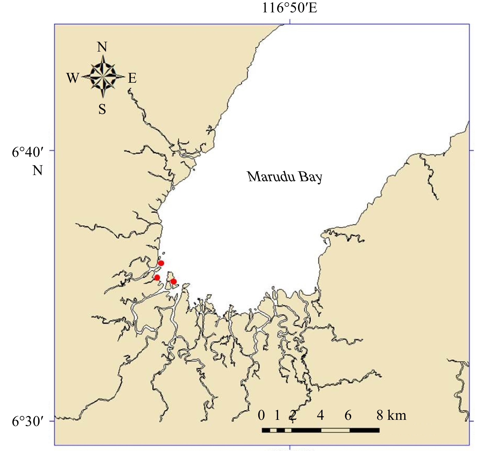
1.
Samples of blood cockle were collected in the inner region of the Marudu Bay (marked by red dots).
| Citation: | Tingting Sun, Lei Wang, Jianmin Zhao, Zhijun Dong. Application of DNA metabarcoding to characterize the diet of the moon jellyfish Aurelia coerulea polyps and ephyrae[J]. Acta Oceanologica Sinica, 2021, 40(8): 160-167. doi: 10.1007/s13131-021-1800-8

|
Blood cockle, Tegillarca granosa (Linnaeus, 1758), formerly known as Anadara granosa is a bivalvia under the Arcidae family. It inhabits soft muddy bottoms of tidal flats formed in estuaries or interior of bays (Nakao et al., 1989) and known to be widely distributed from the Middle East to East Asia (Faulkner, 2010). In Malaysia, T. granosa is naturally found in Penang, Perak, Selangor (Pathansali and Song, 1958) and Johor (Yurimoto et al., 2014). Moreover, according to Hamli et al. (2012), the bivalve is also found in Sarawak particularly in Kuching and Bintulu regions.
T. granosa is a major fishery in the Malaysia’s inshore waters, contributing over 50% to national aquaculture production (Sugiyama et al., 2004) and dominating 93% of total shellfish species production (Department of Fisheries Malaysia, 2013). In 2002, Malaysia was ranked 5th in Asia Pacific in the production of T. granosa with 78 712 tons (Sugiyama et al., 2004). Since the first commercial exploitation in Perak in 1948, this species has been cultivated extensively on several mudflats on Malaysia’s west coast such as Kedah (Merbok), Pulau Pinang (Juru), Perak (Kuala Gula, Kuala Sangga-Matang, Kuala Trong, Sg.Jarum), Selangor (Kuala Selangor) and Johor (Muar) (Mirzaei et al., 2015). There is no direct evidence in the literature on the distribution of T. granosa in Sabah. However, based on our observation, this species occurs in three areas namely Marudu Bay (North Eastern Sabah), Labuk Bay and Tawau (Eastern Sabah) in Sabah. Moreover, our observation also indicated that fewer cockles are being caught by fishers every year. This situation is alarming as the cockle resource in the bay may not be able to sustain unless an intervention is carried out to sustainably manage its natural stock.
Population parameter assessments are important for an effective management of the fishery. A number of similar studies on population dynamics of this species have been conducted in Kuala Juru, Kuala Sepetang, Sungai Besar Selangor (Oon, 1986), Sungai Buloh (Broom, 1982), and Balik Pulau (Mirzaei et al., 2015) in Malaysia as well as in other countries in Kakinada Bay, India (Narasimham, 1988b), Ang Sila, Thailand (Vakily, 1992), and Desa Menco, Kecamatan Wedung dan Demak in Indonesia (Imtihan et al., 2014). Despite the extensive literature of this topic, information on the occurrence and the distribution of this species in Northeast Malaysian Borneo (Sabah) is still scarce. Therefore, this study is established to acquire baseline information regarding the population dynamics and the level of exploitation on the natural stock of this species in the Marudu Bay.
Marudu Bay (6°35′–7°00′N, 116°45′–117°00′E) is situated within the Tun Mustapha Marine Park (Fig. 1), the largest marine protected area on the northeast Borneo. Monthly samplings were conducted from July 2017 to June 2018. Samples of T. granosa (Fig. 2) in an area of 500 m2 (50 m×10 m) were hand collected. A total of 279 specimens were obtained throughout the study period (Table 1). Shell length (anterior-posterior) of each specimen was measured with accuracy of 0.1 mm using Vernier calipers (Mitutoyo, Shah Alam, Malaysia). The total weight was recorded using an electronic balance to the nearest 0.01 g.

| Midlength/mm | Jul. 2017 | Aug. 2017 | Sept. 2017 | Oct. 2017 | Nov. 2017 | Dec. 2017 | Jan. 2018 | Feb. 2018 | Mar. 2018 | Apr. 2018 | May 2018 | Jun. 2018 |
| 27.5 | 1 | 0 | 0 | 0 | 0 | 0 | 0 | 0 | 0 | 0 | 0 | 0 |
| 32.5 | 4 | 0 | 0 | 0 | 0 | 0 | 0 | 0 | 0 | 0 | 0 | 0 |
| 37.5 | 3 | 0 | 1 | 0 | 0 | 0 | 0 | 0 | 0 | 0 | 0 | 1 |
| 42.5 | 0 | 1 | 1 | 0 | 1 | 0 | 1 | 0 | 2 | 0 | 0 | 1 |
| 47.5 | 4 | 0 | 3 | 0 | 7 | 2 | 3 | 3 | 2 | 1 | 0 | 1 |
| 52.5 | 27 | 8 | 1 | 4 | 5 | 4 | 3 | 4 | 3 | 4 | 1 | 4 |
| 57.5 | 9 | 1 | 3 | 5 | 8 | 0 | 4 | 7 | 7 | 5 | 3 | 9 |
| 62.5 | 5 | 6 | 4 | 3 | 5 | 4 | 2 | 8 | 2 | 2 | 4 | 9 |
| 67.5 | 2 | 4 | 5 | 1 | 9 | 2 | 1 | 4 | 3 | 0 | 2 | 3 |
| 72.5 | 0 | 0 | 1 | 0 | 7 | 0 | 0 | 0 | 0 | 1 | 1 | 1 |
| 77.5 | 0 | 0 | 1 | 1 | 2 | 0 | 0 | 0 | 0 | 0 | 0 | 0 |
| 82.5 | 0 | 0 | 0 | 0 | 1 | 1 | 0 | 0 | 0 | 0 | 0 | 0 |
| Total | 55 | 20 | 20 | 14 | 45 | 13 | 14 | 26 | 19 | 13 | 11 | 29 |
| Note: 0 represents no cockle found. | ||||||||||||
 DownLoad:
CSV
DownLoad:
CSV
The monthly 5 mm intervals of shell length frequency distribution data of cockle specimens were used to estimate the growth parameters (L∞, K, ϕ), mortality (Z, M, F), exploitation (E) and recruitment of the species in the Marudu Bay using the FAO-ICLARM Stock Assessment Tools (FiSAT) computer package (Gayanilo et al., 2005).
Five random specimens of blood cockles were collected each month and were used for condition index (CI) analysis during the experimental period (12 months). Briefly, the cockle specimens were dissected to separate meat from the shell. Then, the meats and the empty shells were completely dried in drying oven (Memmert, Büchenbach, Germany). The condition index was then calculated based on the ratio of the dry meat weight (DW) and the shell weight (SW) following Davenport and Chen (1987) as follows:
| $$ {\rm{CI }}\! \!=\!\! {\rm{ }}\left({{\rm{DW}}/{\rm{SW}}} \right){\rm{ }}\!\! \times\!\! {\rm{ }}100. $$ | (1) |
The monthly condition indices were analysed using the SPSS Windows Statistical Package (version 21, Chicago, IL, USA). The tests were judged to be significant at p<0.05 level. Prior to analyses, all variables were tested for normality and homogeneity of variances.
The relationship of W = aLb, where W is the weight (g) and L is the length (mm) of T. granosa, a is the intercept (condition factor) and b is the slope (growth coefficient) was used to establish the length-weight relationship (Quinn II and Deriso, 1999). The a and b parameters were calculated using regression analysis of log-log transformed data:
| $$ {\rm{log}}_{10}W = {\rm{ log}}_{10}a + b{\rm{log}}_{10}L. $$ | (2) |
The correlation (R2), which is the level of relationship between the length and weight, was calculated from the linear analysis. If b = 3.0, growth is isometric, however if b>3.0, growth is positive allometric. Growth is negative allometric when b<3.0.
The asymptotic length (L∞) and the growth coefficient (K) of the von Bertalanffy growth function (VBGF) of the cockle stock were estimated by means of ELEFAN 1 (Pauly and David, 1981). The inverse von Bertalanffy growth equation (Sparre and Venema, 1992) was used to estimate the average length of the cockle at certain age by the equation:
| $$ {L}_{t}={L}_{\infty }\left[1-{{\rm{e}}}^{-K\left(t-{t}_{0}\right)}\right]{\rm{,}} $$ | (3) |
where Lt is the mean length at age t and t0 is the hypothetical age at which the length is zero (Newman, 2002). The t0 value was predicted by using Pauly (1983) equation as follows:
| $$ \mathrm{log}_{10}\left(-{t}_{0}\right)=-0.392\;2-0.275\;2{\mathrm{log}}_{10}{L}_{\infty }-1.038{\mathrm{log}}_{10}K. $$ | (4) |
The potential longevity (tmax) of the cockles was procured using the Pauly (1983) formula tmax=3/K. The growth performance index (ϕ) was then estimated by using the estimated L∞ and K values (Pauly and Munro, 1984) based on the following equation:
| $$ \phi = {\rm{ }}2{\rm{lo}}{{\rm{g}}_{10}}{L_\infty } + {\rm{ lo}}{{\rm{g}}_{10}}K. $$ | (5) |
The recruitment rates were obtained by backward projection on the length axis of a set of available length-frequency data as described in FiSAT routine (Pauly and David, 1981).
Total mortality (Z) is comprised of two components: natural mortality (M); mortality due to predation, disease, etc., and fishing mortality (F); mortality due to harvesting by humans. The total mortality (Z) was estimated by the length converted catch curve method (Pauly and Munro, 1984) and fishing mortality (F) was estimated by the following equation:
| $$ F = Z - M. $$ | (6) |
The exploitation level (E) was then estimated based on the equation described by Gulland (1965) as follows:
| $$ E=F/\left(F+M\right). $$ | (7) |
Relative yield per recruit (Y'/R) and biomass per recruit (B'/R) were estimated according to the model of Beverton and Holt (1993) using the knife-edge selection.
The condition indices of the blood cockle (T. granosa) in the Marudu Bay ranged from 3.05 to 7.17 with a mean (±SD) of 4.98±0.86 (Fig. 3). The maximum values occurred in July followed by a steady decline in October and further decrease to the minimum levels in February. However, no significant difference (p>0.05) was observed in condition indices throughout the study period.

The length and weight of T. granosa ranged 27.7–82.2 mm and 13.11–192.7 g, respectively. The calculated length-weight relationship equation was log10W=2.681 7log10L − 0.17816, R2=0.9501. The exponential form of the equation was W=0.6635L2.6817 (R2=0.9501) which was found by plotting the length values against weight (Fig. 4). The computed growth coefficient (b) was 2.6 at 95% confidence limit.

The growth parameters (L∞, K, t0) are useful in assessing the growth rates between and within individuals inhabiting various environments. The estimated asymptotic length (L∞) of the T. granosa was 86.68 mm and the growth coefficient (K) was 0.98 a–1. The estimated t0 was −0.1212 for T. granosa in the Marudu Bay. The computer growth curve using these parameters is shown over the restructured length distribution based on the length-frequency data (Fig. 5).

The observed maximum shell length of T. granosa in the Marudu Bay was 82.55 mm and the predicted maximum shell length was 84.44 mm (Fig. 6). The confidence interval was 79.29 mm to 89.58 mm (95% probability of occurrence). The mean lengths of T. granosa in the Marudu Bay were estimated to be 21.31 mm, 31.16 mm, 39.53 mm, 46.63 mm, 52.67 mm and 57.79 mm at the end of 2, 4, 6, 8, 10 and 12 months of age, respectively. The best estimated value of K was 0.98 a–1 (Fig. 7) and the growth performance index (ϕ) was 3.87. The estimated maximum life span (tmax) was 3.06 years, which showed that T. granosa is a short-lived species.


The recruitment of T. granosa in the Marudu Bay occurred throughout the year with two apparent peaks, one is in March and another is in October (Fig. 8). The percent recruitment varied from 1.2% to 19.75% during the 1-year study. The highest and lowest percent recruitment was observed in October and August. More than 38% of the total recruitment was contributed by the spawning peaks in March and October.

The total mortality of the blood cockle in the Marudu Bay was estimated at 2.39 a–1. The mean annual seawater temperature (28.4°C) was used to calculate the natural mortality in study site. Natural events and fishing activities were estimated to contribute the mortality at the rate of 1.32 a–1 and 1.07 a–1, respectively (Fig. 9). Meanwhile, the estimated exploitation level (E) of the cockle in Marudu Bay was at 0.45. Figure 10 shows the results of the relative Y'/R and B'/R analysis for T. granosa using two types of selection curves. The computed maximum allowable limit of exploitation (Emax) for the Y'/R and B'/R was 0.395.


Condition index (CI) is often used to characterize flesh quality or the apparent condition of a stock under a given environmental condition (Li et al., 2009). The values of condition index can be generally divided into three fatness categories (CI≤2 (thin); CI=2 to 4 (moderate); CI≥4 (fat)) (Davenport and Chen, 1987). In the present study it was noted that the condition index of the blood cockles in the Marudu Bay was estimated at 4.98±0.86 which fell within the fat category. This value was higher than that of the same species recorded in the Kakinada Bay, India (Narasimham, 1988a) (Table 2) but much lower than those occurred in the Straits of Malacca, Malaysia (Khalil et al., 2017) and Black Sea Coast, Turkey (Sahin et al., 2006).
| Location | Species | Condition index (±SD) | Reference |
| Marudu Bay, Malaysia | Tegillarca granosa | 4.98±0.86 | current study |
| Straits of Malacca, Malaysia | Anadara granosa | 6.76±1.13 | Khalil et al. (2017) |
| Black Sea Coast, Turkey | A. granosa | 7.88±1.80 | Sahin et al. (2006) |
| Kakinada Bay, India | A. granosa | 4.11 | Narasimham (1988a) |
DownLoad:
CSV
The influence of environmental conditions such as temperature (Freites et al., 2010; Khalil, 2013), salinity (Engle, 1958), seasonal variations (Rebelo et al., 2005; Sahin et al., 2006), chemical property of the water and the sediment (Engle, 1958), population density, availability of food (Korringa, 1952; Galtsoff, 1965) and different pollutants have on bivalves can be evaluated using the CI (Lawrence and Scott, 1982; Scott and Lawrence, 1982; Rosas et al., 1983; Marcus et al., 1989). The CI can be used as a tool to determine the ecophysiological influences that affect the physiological changes which suffered by the bivalves in the forms of carbohydrate, glycogen and protein fractions, and also lipid and mineral contents (Mercado-Silva, 2005). In the previous studies, the correlations between CI and phytoplankton biomass were shown apparent in Anadara inaequivalvis (Sahin et al., 2006), Laternula elliptica (Kang et al., 2009) and Fulvia fragilis (Rifi et al., 2015). Besides, previous studies also showed correlation between CI and sea temperature in Cerastoderma edule (Ong et al., 2017) and F. fragilis (Rifi et al., 2015).
Based on the estimation from the length-weight relationship, the growth coefficient b generally lies between 2.5 and 3.5. The growth coefficient b is a shape parameter to determine the body form of the species (Kuriakose, 2017). The relation is said to be isometric when it is equal to 3 (Carlander, 1997). In isometric growth, every part of the organism’s body grows at the same rate while in allometric growth the proportions of organism’s body parts grow at different rate manner in which the length was growing faster than the weight. The growth coefficient b value (2.6) in the current study was smaller than the isometric value (b=3). Therefore, the value of b in the current study demonstrates that T. granosa grows negative allometrically (length was growing faster than the weight) instead of isometrically.
In addition, b value of the current study (2.6) was higher than those reported in the Balik Pulau, Malaysia (2.33) (Mirzaei et al., 2015) and Kakinada Bay, India (2.12) (Narasimham, 1988b) but lower than those reported in the Phuket, Thailand (3.04) (Boonruang and Janekarn, 1983) and Sungai Buloh, Malaysia (3.37) (Broom, 1982) (Table 3). The different values may be due to the influence of biological and ecological factors such as the availability of food (Fréchette et al., 1992; Nakaoka, 1992), water temperature, density and shore level (Hickman, 1979).
| Location | Species | a | b | Reference |
| Marudu Bay, Malaysia | Tegillarca granosa | 0.664 | 2.60 | current study |
| Balik Pulau, Malaysia | Anadara granosa | 0.002 | 2.33 | Mirzaei et al. (2015) |
| Sungai Buloh, Malaysia | A. granosa | 0.240 | 3.37 | Broom (1982) |
| Kakinada Bay, India | A. granosa | 0.260 | 2.12 | Narasimham (1988b) |
| Thailand | A. granosa | 0.360 | 3.04 | Boonruang and Janekarn (1983) |
| Note: a is the intercept (condition factor) and b is the slope (growth coefficient). | ||||
DownLoad:
CSV
The asymptotic length (L∞) of T. granosa in the Marudu Bay (86.68 mm) was higher compared to species occurring in other places: Malaysia (35.4 mm to 45 mm) (Mirzaei et al., 2015; Broom, 1982; Oon, 1986), India (73.4 mm) (Narasimham, 1988b) and Thailand (36.9 mm) (Vakily, 1992) but lower than the one reported in the Indonesia (106.8 mm to 129.9 mm) (Imtihan et al., 2014) (Table 4). The growth coefficient value, K for the cockles in the Marudu Bay (0.98 a–1) which describes how quickly the maximum length is attained was higher than those recorded in other places (0.06 a–1 to 0.88 a–1) with exception to Balik Pulau, Malaysia (1.1 a–1) (Mirzaei et al., 2015), Sungai Buloh, Malaysia (1.01 a–1) (Broom, 1982) and Ang Sila, Thailand (1.86 a–1) (Vakily, 1992).
| Location | Species | L∞/mm | K/a–1 | F/a–1 | E | Reference |
| Marudu Bay, Malaysia | Tegillarca granosa | 86.68 | 0.98 | 1.07 | 0.45 | current study |
| Balik Pulau, Malaysia | Anadara granosa | 35.4 | 1.1 | 0.48 | 0.16 | Mirzaei et al.(2015) |
| Kuala Juru, Malaysia | A. granosa | 45 | 0.55 | 2.69 | 0.83 | Oon (1986) |
| Kuala Sepetang, Malaysia | A. granosa | 40.5 | 0.79 | 3.33 | 0.81 | Oon (1986) |
| Sungai Besar Selangor, Malaysia | A. granosa | 41.4 | 0.78 | 2.88 | 0.79 | Oon (1986) |
| Pulau Sangga, Malaysia | A. granosa | 37.2 | 0.88 | 2.05 | 0.7 | Oon (1986) |
| Sungai Buloh, Malaysia | A. granosa | 44.4 | 1.01 | – | – | Broom (1982) |
| Kakinada Bay, India | A. granosa | 73.4 | 0.58 | – | – | Narasimham (1988b) |
| Ang Sila, Thailand | A. granosa | 36.9 | 1.86 | – | – | Vakily (1992) |
| Desa Menco, Indonesia | A. granosa | 129.9 | 0.07 | – | – | Imtihan et al. (2014) |
| Kecamatan Wedung, Indonesia | A. granosa | 112.1 | 0.07 | – | – | Imtihan et al. (2014) |
| Demak, Indonesia | A. granosa | 106.8 | 0.06 | – | – | Imtihan et al. (2014) |
| Note: L∞: estimated asymptotic length; K: growth coefficient; F: estimated fishing mortality; E: estimated exploitation level. | ||||||
DownLoad:
CSV
Environmental conditions and population crowding have known to negatively influence the growth of blood cockles (Broom, 1985; Tiensongrusmee and Pontjoprawiro, 1988). Substrate, salinity, dissolved oxygen, slope of the muddy flat where the cockles are seeded and the food availability are among the main environmental factors known to affect the growth of blood cockles (Broom, 1985; Gosling, 2003). The productivity and the growth rate of mollusc species can be restricted by extreme differences in salinity, increase exposure period of the muddy flat, and population density of cockles (Broom, 1985, Davenport and Wong, 1986).
The estimated maximum life span (tmax) was 3.06 years, for the blood cockle T. granosa in the Marudu Bay, Sabah. The present findings seem to be consistent with Mirzaei et al. (2015) in the Balik Pulau, Penang Island (2.72 years) and Narasimham (1969) in the Kakinada Bay, India (3 years) which showed that T. granosa is a short-lived species.
The current study demonstrated that the recruitment of T. granosa in the Marudu Bay occurs all year round, with two seasonal pulse producing two cohorts per year (March and October) and the highest peak occurs in October. This finding is in agreement with major spawning season reported from previous research (Table 5) and is backed up by the evidence in Khalil et al. (2017) through which the author reported that Anadara granosa spawn in February to March and October in the Pulau Pinang, Malaysia, September to October in the Banda Aceh and Lhokseumawe, Indonesia. Further studies using environmental variables are recommended to explain spawning and recruitment patterns.
| Location | Species | Spawning period | Reference |
| Marudu bay, Malaysia | Tegillarca granosa | March to April and September to October | current study |
| Pulau Pinang, Malaysia | Anadara granosa | February to March and October | Khalil et al. (2017) |
| Pulau Pinang, Malaysia | A. granosa | August to September | Broom (1983) |
| Selangor, Malaysia | A. granosa | September and November | Broom (1983) |
| Phuket, Thailand | A. granosa | October to November | Boonruang and Janekarn (1983) |
| Pattani Bay, Thailand | A. granosa | September and December | Suwanjarat et al. (2009) |
| Banda Aceh, Indonesia | A. granosa | September to October | Khalil et al. (2017) |
| Lhokseumawe, Indonesia | A. granosa | September to October | Khalil et al. (2017) |
DownLoad:
CSV
Mortality and exploitation level are important parameters to understand the dynamic population of cockles (Mirzaei et al., 2015). Recommended exploitation rate of 0.5 has been suggested by Gulland (1984) as a sustainable exploitation, where the fishing mortality is equal to natural mortality. In the current study, the higher natural mortality (M=1.32 a–1) compared to the fishing mortality (F=1.07 a–1) rate indicated the unbalance position of the stock. The exploitation rate of 0.45 which is below the recommended exploitation rate of 0.5 suggesting that natural events were the major cause of death among cockles in the Marudu Bay.
However, the estimated maximum allowable limit of exploitation rate (Emax) giving maximum relative Y'/R was 0.395, which was very well below the actual exploitation rates of 0.45. Thus, the cockle stock in the Marudu Bay appears to be overexploited in terms of Y'/R and B'/R. This is confirmed by the local’s scarcity observation of cockles at the areas close to the villages and that the fishers tended to explore areas far from the common fishing grounds to get a good catch.
The result of the current study was in accordance with the findings of other studies conducted in Malaysia such as Kuala Juru, Kuala Sepetang, Sangga Besar and Sungai Buloh (0.7 to 0.83) (Oon, 1986), where the exploitation rates of T. granosa were above the recommended sustainable exploitation rate of 0.5. These high exploitation levels could have been attributed to the high market demand of T. granosa in the Peninsular Malaysia (Mirzaei et al., 2015). Through this analysis, the need of decreasing fishing effort corresponding fishing mortality has been made evident. An alternative to this is to carry out a sustainable fishery management.
These scientific information on population dynamics and condition index of cockle derived from the current study can be utilized for establishing sustainable fishery management strategies for natural stocks of blood cockle in the Marudu Bay. Dynamic population models can be designed to provide management authorities an indication of the bay’s carrying capacity (Dame, 1993) as the aim of a sustainable fishery management is the estimation of the area’s carrying capacity (National Research Council, 2010). Carrying capacity can be described in terms of a system’s physical environment, output yield and ecological condition, as well as local social and cultural structures tolerance (National Research Council, 2010). Estimating the capacity carrying system has focused largely on determining the carrying capacity output, which is the maximum sustainable yield that can be produced within a region (McKindsey et al., 2006). By understanding the maximum sustainable yield, it will help to determine how much resources can be harvested from sea without further depletion.
Besides, strategies such as size restriction for harvesting, close season for fishing, restricted fishing zone and use of non-destructive fishing gear can also be implemented in carrying out sustainable fishery management. However, these management strategies should take into consideration the economic aspects of fishermen communities as the farmers are more concerned with short-term economic benefits or meeting the demands of their daily needs (Santoso et al., 2015). This fact can be supported by the past event whereby the involvement of government to stabilize the industry and to prevent overexploitation of the cockle population was met with much resistance from the cockle farmers. The dropped production of cockles from an all-time high of 120 000 tonnes in 1980 to 40 000 tonnes in 1983 and the increased of spats’ prices to more than double from 1919 to 1980 had caused the government to enforce minimum catch size of 31.8 mm and a ban on the exports of spats. However, the implementation of the minimum catch size of 31.8 mm has experienced much objections from the cockle farmers since they considered the size is too large for feasible culture operations (Oon, 1986).
Therefore, more viable management strategy is suggested by practising cohesive interaction in responsible blood cockle fisheries management. In this interaction, local farmers’ participation in management is incorporated in creating sustainable livelihoods and promoting integrated management towards sustainable fisheries (De Young et al., 2008). The local farmers will be able to earn income by collecting blood cockles and selling them to markets in terms of livelihood sustainability while practicing sea ranching strategy by rearing juveniles’ blood cockle caught and allowing blood cockle to breed in the wild before marketed. This sea ranching strategy is helpful in developing aquaculture for replenishing cockle stocks and at the same time allowing farmers to gain both caught and aquaculture productions for economic benefits (Santoso et al., 2015). Besides, it is also important to practice integrated management approach by conserving the mangrove forests and conducting surveillance on the irresponsible fishing practiced in the area to ensure the sustainability of this blood cockle fisheries (Suanrattanachai et al., 2011).
The current study demonstrated T. granosa population in the Marudu Bay grew in negative allometric fashion. However, it has a satisfactory condition index and recruitment. Although it reproduces continuously throughout the year, the exploitation level was approaching the maximum exploitation level that if it is not managed sustainably, it could lead to population collapse. Hence, fishing the natural stock of the cockle in the Marudu Bay requires sustainable management plan by involving local farmers in practicing integrated management approach such as sea ranching program, conservation of mangrove forests and surveillance on irresponsible fishing.
| [1] |
Albaina A, Aguirre M, Abad D, et al. 2016. 18S rRNA V9 metabarcoding for diet characterization: a critical evaluation with two sympatric zooplanktivorous fish species. Ecology and Evolution, 6(6): 1809–1824. doi: 10.1002/ece3.1986
|
| [2] |
Arai M N. 1997. A Functional Biology of Scyphozoa. London, UK: Chapman & Hall, 58–91
|
| [3] |
Ballard J W O, Melvin R G. 2010. Linking the mitochondrial genotype to the organismal phenotype. Molecular Ecology, 19(8): 1523–1539. doi: 10.1111/j.1365-294X.2010.04594.x
|
| [4] |
Båmstedt U. 1990. Trophodynamics of the scyphomedusae Aurelia aurita. Predation rate in relation to abundance, size and type of prey organism. Journal of Plankton Research, 12(1): 215–229. doi: 10.1093/plankt/12.1.215
|
| [5] |
Båmstedt U, Wild B, Martinussen M. 2001. Significance of food type for growth of ephyrae Aurelia aurita (Scyphozoa). Marine Biology, 139(4): 641–650. doi: 10.1007/s002270100623
|
| [6] |
Bayha K M, Dawson M N. 2010. New family of allomorphic jellyfishes, Drymonematidae (Scyphozoa, Discomedusae), emphasizes evolution in the functional morphology and trophic ecology of gelatinous zooplankton. The Biological Bulletin, 219(3): 249–267. doi: 10.1086/BBLv219n3p249
|
| [7] |
Bohmann K, Monadjem A, Noer C L, et al. 2011. Molecular diet analysis of two African free-tailed bats (Molossidae) using high throughput sequencing. PLoS ONE, 6(6): e21441. doi: 10.1371/journal.pone.0021441
|
| [8] |
Brassea-Pérez E, Schramm Y, Heckel G, et al. 2019. Metabarcoding analysis of the Pacific harbor seal diet in Mexico. Marine Biology, 166(8): 106. doi: 10.1007/s00227-019-3555-8
|
| [9] |
Caporaso J G, Kuczynski J, Stombaugh J, et al. 2010. QIIME allows analysis of high-throughput community sequencing data. Nature Methods, 7(5): 335–336. doi: 10.1038/nmeth.f.303
|
| [10] |
Cardona L, de Quevedo I Á, Borrell A, et al. 2012. Massive consumption of gelatinous plankton by Mediterranean apex predators. PLoS ONE, 7(3): e31329. doi: 10.1371/journal.pone.0031329
|
| [11] |
Cardona L, Martínez-Iñigo L, Mateo R, et al. 2015. The role of sardine as prey for pelagic predators in the western Mediterranean Sea assessed using stable isotopes and fatty acids. Marine Ecology Progress Series, 531: 1–14. doi: 10.3354/meps11353
|
| [12] |
Carrizo S S, Schiariti A, Nagata R M, et al. 2016. Preliminary observations on ephyrae predation by Lychnorhiza lucerna medusa (Scyphozoa; Rhizostomeae). Der Zoologische Garten, 85(1–2): 74–83. doi: 10.1016/j.zoolgart.2015.09.011
|
| [13] |
Cavalier-Smith T. 1998. A revised six-kingdom system of life. Biological Reviews of the Cambridge Philosophical Society, 73: 203–266. doi: 10.1017/s0006323198005167
|
| [14] |
Costello J H, Colin S P, Dabiri J O. 2008. Medusan morphospace: phylogenetic constraints, biomechanical solutions, and ecological consequences. Invertebrate Biology, 127(3): 265–290. doi: 10.1111/j.1744-7410.2008.00126.x
|
| [15] |
Dawson M N, Gupta A S, England M H. 2005. Coupled biophysical global ocean model and molecular genetic analyses identify multiple introductions of cryptogenic species. Proceedings of the National Academy of Sciences of the United States of America, 102(34): 11968–11973. doi: 10.1073/pnas.0503811102
|
| [16] |
Deagle B E, Chiaradia A, McInnes J, et al. 2010. Pyrosequencing faecal DNA to determine diet of little penguins: is what goes in what comes out?. Conservation Genetics, 11(5): 2039–2048. doi: 10.1007/s10592-010-0096-6
|
| [17] |
Dong Zhijun. 2019. Blooms of the moon jellyfish Aurelia: causes, consequences and controls. In: Sheppard C, ed. World Seas: An Environmental Evaluation. 2nd ed. Amsterdam, the Netherlands: Elsevier, 163–171, doi: 10.1016/B978-0-12-805052-1.00008-5
|
| [18] |
Dong Zhijun, Liu Dongyan, Keesing J K. 2010. Jellyfish blooms in China: dominant species, causes and consequences. Marine Pollution Bulletin, 60(7): 954–963. doi: 10.1016/j.marpolbul.2010.04.022
|
| [19] |
Dong Zhijun, Liu Dongyan, Keesing J K. 2014. Contrasting trends in populations of Rhopilema esculentum and Aurelia aurita in Chinese waters. In: Pitt K A, Lucas C H, eds. Jellyfish Blooms. Dordrecht, the Netherlands: Springer, 207–218, doi: 10.1007/978-94-007-7015-7_9
|
| [20] |
Dong Zhijun, Liu Zhongyuan, Liu Dongyan. 2015. Genetic characterization of the scyphozoan jellyfish Aurelia spp. in Chinese coastal waters using mitochondrial markers. Biochemical Systematics and Ecology, 60: 15–23. doi: 10.1016/j.bse.2015.02.018
|
| [21] |
Duarte C M, Pitt K A, Lucas C H, et al. 2013. Is global ocean sprawl a cause of jellyfish blooms?. Frontiers in Ecology and the Environment, 11(2): 91–97. doi: 10.1890/110246
|
| [22] |
Ficetola G F, Coissac E, Zundel S, et al. 2010. An In silico approach for the evaluation of DNA barcodes. BMC Genomics, 11: 434. doi: 10.1186/1471-2164-11-434
|
| [23] |
Graham W M, Kroutil R M. 2001. Size-based prey selectivity and dietary shifts in the jellyfish, Aurelia aurita. Journal of Plankton Research, 23(1): 67–74. doi: 10.1093/plankt/23.1.67
|
| [24] |
Gröndahl F. 1988. Interactions between polyps of Aurelia aurita and planktonic larvae of scyphozoans: an experimental study. Marine Ecology-Progress Series, 45: 87–93. doi: 10.3354/meps045087
|
| [25] |
Gröndahl F. 1989. Evidence of gregarious settlement of planula larvae of the scyphozoan Aurelia aurita: an experimental study. Marine Ecology-Progress Series, 56: 119–125. doi: 10.3354/meps056119
|
| [26] |
Han C H, Uye S I. 2010. Combined effects of food supply and temperature on asexual reproduction and somatic growth of polyps of the common jellyfish Aurelia aurita s.l. Plankton and Benthos Research, 5(3): 98–105. doi: 10.3800/pbr.5.98
|
| [27] |
Higgins III J E, Ford M D, Costello J H. 2008. Transitions in morphology, nematocyst distribution, fluid motions, and prey capture during development of the scyphomedusa Cyanea capillata. The Biological Bulletin, 214(1): 29–41. doi: 10.2307/25066657
|
| [28] |
Hirai J, Hidaka K, Nagai S, et al. 2017. Molecular-based diet analysis of the early post-larvae of Japanese sardine Sardinops melanostictus and Pacific round herring Etrumeus teres. Marine Ecology Progress Series, 564: 99–113. doi: 10.3354/meps12008
|
| [29] |
Hu Simin, Guo Zhiling, Li Tao, et al. 2015. Molecular analysis of in situ diets of coral reef copepods: evidence of terrestrial plant detritus as a food source in Sanya Bay, China. Journal of Plankton Research, 37(2): 363–371. doi: 10.1093/plankt/fbv014
|
| [30] |
Huang Yousong. 2013. PCR-based in situ dietary analysis of two common copepods in Bohai Sea and Yellow Sea coastal waters (in Chinese)[dissertation]. Qingdao: Ocean University of China
|
| [31] |
Jarman S N, McInnes J C, Faux C, et al. 2013. Adélie penguin population diet monitoring by analysis of food DNA in scats. PLoS ONE, 8(12): e82227. doi: 10.1371/journal.pone.0082227
|
| [32] |
Kamiyama T. 2013. Planktonic ciliates as food for the scyphozoan Aurelia aurita (s.l.): effects on asexual reproduction of the polyp stage. Journal of Experimental Marine Biology and Ecology, 445: 21–28. doi: 10.1016/j.jembe.2013.03.018
|
| [33] |
Kamiyama T. 2018. Planktonic ciliates as food for the scyphozoan Aurelia coerulea: feeding and growth responses of ephyra and metephyra stages. Journal of Oceanography, 74: 53–63. doi: 10.1007/s10872-017-0438-9
|
| [34] |
Kodama T, Hirai J, Tamura S, et al. 2017. Diet composition and feeding habits of larval Pacific bluefin tuna Thunnus orientalis in the Sea of Japan: integrated morphological and metagenetic analysis. Marine Ecology Progress Series, 583: 211–226. doi: 10.3354/meps12341
|
| [35] |
Kogovšek T, Bogunović B, Malej A. 2010. Recurrence of bloom-forming scyphomedusae: wavelet analysis of a 200-year time series. Hydrobiologia, 645: 81–96. doi: 10.1007/s10750-010-0217-8
|
| [36] |
Lo W T, Chen I L. 2008. Population succession and feeding of scyphomedusae, Aurelia aurita, in a eutrophic tropical lagoon in Taiwan. Estuarine, Coastal and Shelf Science, 76(2): 227–238. doi: 10.1016/j.ecss.2007.07.015
|
| [37] |
Lucas C H, Graham W M, Widmer C. 2012. Jellyfish life histories: role of polyps in forming and maintaining scyphomedusa populations. Advances in Marine Biology, 63: 133–196. doi: 10.1016/b978-0-12-394282-1.00003-x
|
| [38] |
Magoč T, Salzberg S L. 2011. FLASH: fast length adjustment of short reads to improve genome assemblies. Bioinformatics, 27(21): 2957–2963. doi: 10.1093/bioinformatics/btr507
|
| [39] |
Malej A, Turk V, Lučić D, et al. 2007. Direct and indirect trophic interactions of Aurelia sp. (Scyphozoa) in a stratified marine environment (Mljet Lakes, Adriatic Sea). Marine Biology, 151(3): 827–841. doi: 10.1007/s00227-006-0503-1
|
| [40] |
McInnes J C, Alderman R, Lea M A, et al. 2017. High occurrence of jellyfish predation by black-browed and Campbell albatross identified by DNA metabarcoding. Molecular Ecology, 26(18): 4831–4845. doi: 10.1111/mec.14245
|
| [41] |
O’Rorke R, Lavery S, Chow S, et al. 2012. Determining the diet of larvae of western rock lobster (Panulirus cygnus) using high-throughput DNA sequencing techniques. PLoS ONE, 7(8): e42757. doi: 10.1371/journal.pone.0042757
|
| [42] |
O’Rorke R, Lavery S D, Wang M, et al. 2014. Determining the diet of larvae of the red rock lobster (Jasus edwardsii) using high-throughput DNA sequencing techniques. Marine Biology, 161(3): 551–563. doi: 10.1007/s00227-013-2357-7
|
| [43] |
Östman C. 1997. Abundance, feeding behaviour and nematocysts of scyphopolyps (Cnidaria) and nematocysts in their predator, the nudibranch Coryphella verrucosa (Mollusca). Hydrobiologia, 355(1): 21–28. doi: 10.1023/A:1003065726381
|
| [44] |
Pompanon F, Deagle B E, Symondson W O C, et al. 2012. Who is eating what: diet assessment using next generation sequencing. Molecular Ecology, 21(8): 1931–1950. doi: 10.1111/j.1365-294x.2011.05403.x
|
| [45] |
Purcell J E. 1997. Pelagic cnidarians and ctenophores as predators: selective predation, feeding rates and effects on prey populations. Annales de l'Institute Oceanographique, 73(2): 125–137
|
| [46] |
Purcell J E. 2012. Jellyfish and ctenophore blooms coincide with human proliferations and environmental perturbations. Annual Review of Marine Science, 4: 209–235. doi: 10.1146/annurev-marine-120709-142751
|
| [47] |
Purcell J E, Baxter E J, Fuentes V. 2013. Jellyfish as products and problems of aquaculture. In: Allan G, Burnell G, eds. Advances in Aquaculture Hatchery Technology. Cambridge, UK: Woodhead Publishing, 404–430, doi: 10.1533/9780857097460.2.404
|
| [48] |
Purcell J E, Hoover R A, Schwarck N T. 2009. Interannual variation of strobilation by the scyphozoan Aurelia labiata in relation to polyp density, temperature, salinity, and light conditions in situ. Marine Ecology Progress Series, 375: 139–149. doi: 10.3354/meps07785
|
| [49] |
Purcell J E, Sturdevant M V. 2001. Prey selection and dietary overlap among zooplanktivorous jellyfish and juvenile fishes in Prince William Sound, Alaska. Marine Ecology Progress Series, 210: 67–83. doi: 10.3354/meps210067
|
| [50] |
Riisgård H U, Madsen C V. 2011. Clearance rates of ephyrae and small medusae of the common jellyfish Aurelia aurita offered different types of prey. Journal of Sea Research, 65(1): 51–57. doi: 10.1016/j.seares.2010.07.002
|
| [51] |
Schiariti A, Morandini A C, Jarms G, et al. 2014. Asexual reproduction strategies and blooming potential in Scyphozoa. Marine Ecology Progress Series, 510: 241–253. doi: 10.3354/meps10798
|
| [52] |
Scorrano S, Aglieri G, Boero F, et al. 2017. Unmasking Aurelia species in the Mediterranean Sea: an integrative morphometric and molecular approach. Zoological Journal of the Linnean Society, 180(2): 243–267. doi: 10.1111/zoj.12494
|
| [53] |
Skikne S A, Sherlock R E, Robison B H. 2009. Uptake of dissolved organic matter by ephyrae of two species of scyphomedusae. Journal of Plankton Research, 31(12): 1563–1570. doi: 10.1093/plankt/fbp088
|
| [54] |
Su Maoliang, Liu Huifen, Liang Xuemei, et al. 2018. Dietary analysis of marine fish species: enhancing the detection of prey-specific DNA sequences via high-throughput sequencing using blocking primers. Estuaries and Coasts, 41(2): 560–571. doi: 10.1007/s12237-017-0279-1
|
| [55] |
Sullivan B K, Suchman C L, Costello J H. 1997. Mechanics of prey selection by ephyrae of the scyphomedusa Aurelia aurita. Marine Biology, 130(2): 213–222. doi: 10.1007/s002270050241
|
| [56] |
Thiebot J B, Arnould J P Y, Gómez-Laich A, et al. 2017. Jellyfish and other gelata as food for four penguin species-insights from predator-borne videos. Frontiers in Ecology and the Environment, 15(8): 437–441. doi: 10.1002/fee.1529
|
| [57] |
Titelman J, Hansson L J. 2006. Feeding rates of the jellyfish Aurelia aurita on fish larvae. Marine Biology, 149(2): 297–306. doi: 10.1007/s00227-005-0200-5
|
| [58] |
Tsikhon-Lukanina E A, Reznichenko O G, Lukasheva T A. 1996. Food consumption by scyphistomae of the jellyfish Aurelia aurita in the Black Sea. Oceanology, 35(6): 815–818
|
| [59] |
Uye S I. 2011. Human forcing of the copepod-fish-jellyfish triangular trophic relationship. Hydrobiologia, 666(1): 71–83. doi: 10.1007/s10750-010-0208-9
|
| [60] |
Uye S, Shimauchi H. 2005. Population biomass, feeding, respiration and growth rates, and carbon budget of the scyphomedusa Aurelia aurita in the Inland Sea of Japan. Journal of Plankton Research, 27(3): 237–248. doi: 10.1093/plankt/fbh172
|
| [61] |
Wang Nan, Li Chaolun. 2015. The effect of temperature and food supply on the growth and ontogeny of Aurelia sp. 1 ephyrae. Hydrobiologia, 754(1): 157–167. doi: 10.1007/s10750-014-1981-7
|
| [62] |
Wang Yantao, Zheng Shan, Sun Song, et al. 2015. Effect of temperature and food type on asexual reproduction in Aurelia sp. 1 polyps. Hydrobiologia, 754(1): 169–178. doi: 10.1007/s10750-014-2020-4
|
| [63] |
Zheng Shan, Sun Xiaoxia, Wang Yantao, et al. 2015. Significance of different microalgal species for growth of moon jellyfish ephyrae, Aurelia sp.1. Journal of Ocean University of China, 14(5): 823–828. doi: 10.1007/s11802-015-2775-x
|
| [64] |
Zoccarato L, Celussi M, Pallavicini A, et al. 2016. Aurelia aurita ephyrae reshape a coastal microbial community. Frontiers in Microbiology, 7: 749. doi: 10.3389/fmicb.2016.00749
|
| 1. | Mawardi Mawardi, M. Ali Sarong, Suhendrayatna Suhendrayatna, et al. Morphometric Analysis and Growth Patterns of Blood Cockle (Tegillarca granosa) in Langsa Mangrove Ecosystems, Indonesia. Grimsa Journal of Science Engineering and Technology, 2024, 2(2): 66. doi:10.61975/gjset.v2i2.55 | |
| 2. | Snigdhodeb Dutta. Population Dynamics of Four Fin Fish Species from a Tropical Estuary. Thalassas: An International Journal of Marine Sciences, 2023, 39(1): 333. doi:10.1007/s41208-023-00527-8 |


Figures(3) / Tables(1)

Supported by:
Beijing Renhe Information Technology Co. Ltd

Joanna W. Doinsing, Vienna Anastasia Admodisastro, Laditah Duisan, Julian Ransangan. Population dynamics and condition index of natural stock of blood cockle, Tegillarca granosa (Mollusca, Bivalvia, Arcidae) in the Marudu Bay, Malaysia[J]. Acta Oceanologica Sinica, 2021, 40(8): 89-97. doi: 10.1007/s13131-021-1791-5

| Midlength/mm | Jul. 2017 | Aug. 2017 | Sept. 2017 | Oct. 2017 | Nov. 2017 | Dec. 2017 | Jan. 2018 | Feb. 2018 | Mar. 2018 | Apr. 2018 | May 2018 | Jun. 2018 |
| 27.5 | 1 | 0 | 0 | 0 | 0 | 0 | 0 | 0 | 0 | 0 | 0 | 0 |
| 32.5 | 4 | 0 | 0 | 0 | 0 | 0 | 0 | 0 | 0 | 0 | 0 | 0 |
| 37.5 | 3 | 0 | 1 | 0 | 0 | 0 | 0 | 0 | 0 | 0 | 0 | 1 |
| 42.5 | 0 | 1 | 1 | 0 | 1 | 0 | 1 | 0 | 2 | 0 | 0 | 1 |
| 47.5 | 4 | 0 | 3 | 0 | 7 | 2 | 3 | 3 | 2 | 1 | 0 | 1 |
| 52.5 | 27 | 8 | 1 | 4 | 5 | 4 | 3 | 4 | 3 | 4 | 1 | 4 |
| 57.5 | 9 | 1 | 3 | 5 | 8 | 0 | 4 | 7 | 7 | 5 | 3 | 9 |
| 62.5 | 5 | 6 | 4 | 3 | 5 | 4 | 2 | 8 | 2 | 2 | 4 | 9 |
| 67.5 | 2 | 4 | 5 | 1 | 9 | 2 | 1 | 4 | 3 | 0 | 2 | 3 |
| 72.5 | 0 | 0 | 1 | 0 | 7 | 0 | 0 | 0 | 0 | 1 | 1 | 1 |
| 77.5 | 0 | 0 | 1 | 1 | 2 | 0 | 0 | 0 | 0 | 0 | 0 | 0 |
| 82.5 | 0 | 0 | 0 | 0 | 1 | 1 | 0 | 0 | 0 | 0 | 0 | 0 |
| Total | 55 | 20 | 20 | 14 | 45 | 13 | 14 | 26 | 19 | 13 | 11 | 29 |
| Note: 0 represents no cockle found. | ||||||||||||
DownLoad:
CSV
| Location | Species | Condition index (±SD) | Reference |
| Marudu Bay, Malaysia | Tegillarca granosa | 4.98±0.86 | current study |
| Straits of Malacca, Malaysia | Anadara granosa | 6.76±1.13 | Khalil et al. (2017) |
| Black Sea Coast, Turkey | A. granosa | 7.88±1.80 | Sahin et al. (2006) |
| Kakinada Bay, India | A. granosa | 4.11 | Narasimham (1988a) |
DownLoad:
CSV
| Location | Species | a | b | Reference |
| Marudu Bay, Malaysia | Tegillarca granosa | 0.664 | 2.60 | current study |
| Balik Pulau, Malaysia | Anadara granosa | 0.002 | 2.33 | Mirzaei et al. (2015) |
| Sungai Buloh, Malaysia | A. granosa | 0.240 | 3.37 | Broom (1982) |
| Kakinada Bay, India | A. granosa | 0.260 | 2.12 | Narasimham (1988b) |
| Thailand | A. granosa | 0.360 | 3.04 | Boonruang and Janekarn (1983) |
| Note: a is the intercept (condition factor) and b is the slope (growth coefficient). | ||||
DownLoad:
CSV
| Location | Species | L∞/mm | K/a–1 | F/a–1 | E | Reference |
| Marudu Bay, Malaysia | Tegillarca granosa | 86.68 | 0.98 | 1.07 | 0.45 | current study |
| Balik Pulau, Malaysia | Anadara granosa | 35.4 | 1.1 | 0.48 | 0.16 | Mirzaei et al.(2015) |
| Kuala Juru, Malaysia | A. granosa | 45 | 0.55 | 2.69 | 0.83 | Oon (1986) |
| Kuala Sepetang, Malaysia | A. granosa | 40.5 | 0.79 | 3.33 | 0.81 | Oon (1986) |
| Sungai Besar Selangor, Malaysia | A. granosa | 41.4 | 0.78 | 2.88 | 0.79 | Oon (1986) |
| Pulau Sangga, Malaysia | A. granosa | 37.2 | 0.88 | 2.05 | 0.7 | Oon (1986) |
| Sungai Buloh, Malaysia | A. granosa | 44.4 | 1.01 | – | – | Broom (1982) |
| Kakinada Bay, India | A. granosa | 73.4 | 0.58 | – | – | Narasimham (1988b) |
| Ang Sila, Thailand | A. granosa | 36.9 | 1.86 | – | – | Vakily (1992) |
| Desa Menco, Indonesia | A. granosa | 129.9 | 0.07 | – | – | Imtihan et al. (2014) |
| Kecamatan Wedung, Indonesia | A. granosa | 112.1 | 0.07 | – | – | Imtihan et al. (2014) |
| Demak, Indonesia | A. granosa | 106.8 | 0.06 | – | – | Imtihan et al. (2014) |
| Note: L∞: estimated asymptotic length; K: growth coefficient; F: estimated fishing mortality; E: estimated exploitation level. | ||||||
DownLoad:
CSV
| Location | Species | Spawning period | Reference |
| Marudu bay, Malaysia | Tegillarca granosa | March to April and September to October | current study |
| Pulau Pinang, Malaysia | Anadara granosa | February to March and October | Khalil et al. (2017) |
| Pulau Pinang, Malaysia | A. granosa | August to September | Broom (1983) |
| Selangor, Malaysia | A. granosa | September and November | Broom (1983) |
| Phuket, Thailand | A. granosa | October to November | Boonruang and Janekarn (1983) |
| Pattani Bay, Thailand | A. granosa | September and December | Suwanjarat et al. (2009) |
| Banda Aceh, Indonesia | A. granosa | September to October | Khalil et al. (2017) |
| Lhokseumawe, Indonesia | A. granosa | September to October | Khalil et al. (2017) |
DownLoad:
CSV
| Midlength/mm | Jul. 2017 | Aug. 2017 | Sept. 2017 | Oct. 2017 | Nov. 2017 | Dec. 2017 | Jan. 2018 | Feb. 2018 | Mar. 2018 | Apr. 2018 | May 2018 | Jun. 2018 |
| 27.5 | 1 | 0 | 0 | 0 | 0 | 0 | 0 | 0 | 0 | 0 | 0 | 0 |
| 32.5 | 4 | 0 | 0 | 0 | 0 | 0 | 0 | 0 | 0 | 0 | 0 | 0 |
| 37.5 | 3 | 0 | 1 | 0 | 0 | 0 | 0 | 0 | 0 | 0 | 0 | 1 |
| 42.5 | 0 | 1 | 1 | 0 | 1 | 0 | 1 | 0 | 2 | 0 | 0 | 1 |
| 47.5 | 4 | 0 | 3 | 0 | 7 | 2 | 3 | 3 | 2 | 1 | 0 | 1 |
| 52.5 | 27 | 8 | 1 | 4 | 5 | 4 | 3 | 4 | 3 | 4 | 1 | 4 |
| 57.5 | 9 | 1 | 3 | 5 | 8 | 0 | 4 | 7 | 7 | 5 | 3 | 9 |
| 62.5 | 5 | 6 | 4 | 3 | 5 | 4 | 2 | 8 | 2 | 2 | 4 | 9 |
| 67.5 | 2 | 4 | 5 | 1 | 9 | 2 | 1 | 4 | 3 | 0 | 2 | 3 |
| 72.5 | 0 | 0 | 1 | 0 | 7 | 0 | 0 | 0 | 0 | 1 | 1 | 1 |
| 77.5 | 0 | 0 | 1 | 1 | 2 | 0 | 0 | 0 | 0 | 0 | 0 | 0 |
| 82.5 | 0 | 0 | 0 | 0 | 1 | 1 | 0 | 0 | 0 | 0 | 0 | 0 |
| Total | 55 | 20 | 20 | 14 | 45 | 13 | 14 | 26 | 19 | 13 | 11 | 29 |
| Note: 0 represents no cockle found. | ||||||||||||
| Location | Species | Condition index (±SD) | Reference |
| Marudu Bay, Malaysia | Tegillarca granosa | 4.98±0.86 | current study |
| Straits of Malacca, Malaysia | Anadara granosa | 6.76±1.13 | Khalil et al. (2017) |
| Black Sea Coast, Turkey | A. granosa | 7.88±1.80 | Sahin et al. (2006) |
| Kakinada Bay, India | A. granosa | 4.11 | Narasimham (1988a) |
| Location | Species | a | b | Reference |
| Marudu Bay, Malaysia | Tegillarca granosa | 0.664 | 2.60 | current study |
| Balik Pulau, Malaysia | Anadara granosa | 0.002 | 2.33 | Mirzaei et al. (2015) |
| Sungai Buloh, Malaysia | A. granosa | 0.240 | 3.37 | Broom (1982) |
| Kakinada Bay, India | A. granosa | 0.260 | 2.12 | Narasimham (1988b) |
| Thailand | A. granosa | 0.360 | 3.04 | Boonruang and Janekarn (1983) |
| Note: a is the intercept (condition factor) and b is the slope (growth coefficient). | ||||
| Location | Species | L∞/mm | K/a–1 | F/a–1 | E | Reference |
| Marudu Bay, Malaysia | Tegillarca granosa | 86.68 | 0.98 | 1.07 | 0.45 | current study |
| Balik Pulau, Malaysia | Anadara granosa | 35.4 | 1.1 | 0.48 | 0.16 | Mirzaei et al.(2015) |
| Kuala Juru, Malaysia | A. granosa | 45 | 0.55 | 2.69 | 0.83 | Oon (1986) |
| Kuala Sepetang, Malaysia | A. granosa | 40.5 | 0.79 | 3.33 | 0.81 | Oon (1986) |
| Sungai Besar Selangor, Malaysia | A. granosa | 41.4 | 0.78 | 2.88 | 0.79 | Oon (1986) |
| Pulau Sangga, Malaysia | A. granosa | 37.2 | 0.88 | 2.05 | 0.7 | Oon (1986) |
| Sungai Buloh, Malaysia | A. granosa | 44.4 | 1.01 | – | – | Broom (1982) |
| Kakinada Bay, India | A. granosa | 73.4 | 0.58 | – | – | Narasimham (1988b) |
| Ang Sila, Thailand | A. granosa | 36.9 | 1.86 | – | – | Vakily (1992) |
| Desa Menco, Indonesia | A. granosa | 129.9 | 0.07 | – | – | Imtihan et al. (2014) |
| Kecamatan Wedung, Indonesia | A. granosa | 112.1 | 0.07 | – | – | Imtihan et al. (2014) |
| Demak, Indonesia | A. granosa | 106.8 | 0.06 | – | – | Imtihan et al. (2014) |
| Note: L∞: estimated asymptotic length; K: growth coefficient; F: estimated fishing mortality; E: estimated exploitation level. | ||||||
| Location | Species | Spawning period | Reference |
| Marudu bay, Malaysia | Tegillarca granosa | March to April and September to October | current study |
| Pulau Pinang, Malaysia | Anadara granosa | February to March and October | Khalil et al. (2017) |
| Pulau Pinang, Malaysia | A. granosa | August to September | Broom (1983) |
| Selangor, Malaysia | A. granosa | September and November | Broom (1983) |
| Phuket, Thailand | A. granosa | October to November | Boonruang and Janekarn (1983) |
| Pattani Bay, Thailand | A. granosa | September and December | Suwanjarat et al. (2009) |
| Banda Aceh, Indonesia | A. granosa | September to October | Khalil et al. (2017) |
| Lhokseumawe, Indonesia | A. granosa | September to October | Khalil et al. (2017) |
 DownLoad:


