Spatial distribution and behavior of dissolved selenium speciation in the South China Sea and Malacca Straits during spring inter-monsoon period

1. Introduction

Selenium (Se) is a vital trace nutrient for the growth of many marine biota, especially primary producers (Araie and Shiraiwa, 2016) due to biological requirement in synthetize of seleno-proteins (Böck et al., 1991; Baines and Fisher, 2001) and cell division (Araie and Shiraiwa, 2016). Selenium limitation can frequently decrease phytoplankton biomass and subsequently constrain the carbon sequestration capability (Wake et al., 2012). Thus, the investigation of Se species is essential for primary production estimation and global carbon cycle (Cutter, 2005; Wake et al., 2012).

Dissolved Se in oceans is defined as dissolved organic selenides (DOSe) and dissolved inorganic Se (DISe, including Se(VI) and Se(IV)) (Fig. 1). Se(IV) and Se(VI) perform a nutrient-like profile from surface ocean to seabed, while DOSe preforms an enrichment in surface and decreases in concentration with depth (Cutter and Cutter, 2001, 1998; Measures et al., 1983; Wambaugh, 2017). Such distribution are the results of intense biological process in euphotic surface layer and multiple regeneration in the deep water (Cutter and Bruland, 1984). Upwelling can introduce Se(IV) and Se(VI) from deep water to surface water (Cutter and Cutter, 1995, 2001; Cutter and Bruland, 1984; Measures et al., 1983; Wambaugh, 2017). Atmosphere deposition and surface loading are frequently assumed to be the major pathway for the transport of terrestrial Se into oceans (Chang et al., 2016; Ibrahim and Al-Farawati, 2017). Se concentrations in surface water are also related with environmental factors in watersheds, e.g. soil composition, temperature and erosion rate (Chang et al., 2020). In addition, anthropogenic activities, such as domestic sewage discharge and petrochemical industry, also deeply influence the land-ocean Se transport process (Duan et al., 2010). Both Se(VI) and Se(IV) can be assimilated by many primary producers, especially with a preference of Se(IV). DOSe inventory in marine systems is under a dynamic balance. On the one hand, decomposition of phytoplankton releases DOSe into the ambient water (Cutter and Cutter, 2001), while DOSe is also consumed as a Se source by several phytoplankton species, especially under the low-level Se(IV) and Se(VI) condition (Baines et al., 2001). Therefore, Se can be rapidly consumed in the surface ocean (euphotic layer) and transferred along food webs (Mason et al., 2018). The assimilation efficiency varies among phytoplankton species (Baines and Fisher, 2001) due to different requirement of Se in their metabolism (Araie and Shiraiwa, 2016). Diatom (e.g. Skeletonema costatum, Thalassiosira oceanica) and Dinophyceae (e.g. Scrippsiella trochoides) frequently host a rapid assimilation rate, while Se utilization by Chlorophyceae is much slower (Baines et al., 2001; Harrison et al., 1988). Therefore, the distribution of Se in oceanic environment, especially in marine upper layer, is commonly linked to composition of phytoplankton communities.

Figure  1.  Sketch of biogeochemical cycle for dissolved Se in oceans (adapted from Cutter and Bruland, 1984; Cutter and Cutter, 1995, 1998, 2001, 2004; Baines and Fisher, 2001; Baines et al., 2001; Wen and Carignan, 2007).

DownLoad: Full-Size Img PowerPoint

As a trace nutrient for biological activities with multiple sources, Se concentration, including Se(VI), Se(IV) and DOSe, markedly varies among different oceans, especially in surface water where sunlight exposure boosts the growth of phytoplankton. For instance, Se(IV) was below 0.01 nmol/L in the Pacific Ocean (20°S–35.67°N) (Cutter and Bruland, 1984). Se(IV) was below 0.03 nmol/L in the north Atlantic Ocean (41.17°–44.55°N) (Measures and Burton, 1980), while increased to range of 0.05 nmol/L to 0.15 nmol/L in the tropical Atlantic Ocean (32.78°S–15.32°N) (Cutter and Cutter, 2001). Few investigation was done in Indian Ocean and Se(IV) was found in the range from 0.03 nmol/L to 0.10 nmol/L (Hattori et al., 2001; Measures et al., 1983). In the Antarctic Ocean, Se(IV) varied at 0.04–0.43 nmol/L (Wake et al., 2012; Xia et al., 1996). Most marine phytoplankton require trace amount (nmol/L level) of Se to maintain their metabolism (Ivanenko, 2018). Then Se is transferred into food chains and involved in the full range of metabolic functions (Ivanenko, 2018), indicating a significance of Se supply on the status and functions of the ecosystem. Previous studies focused much on spatial distribution of Se concentrations in coastal estuaries along a salinity gradient and vertical profile with depth in open oceans (Fig. 2a). However, seldom investigations are done in the Asia monsoon region, particularly in the South China Sea (SCS) and Malacca Straits (MS).

Figure  2.  Stations of Se sampling (a), sea surface height (color shading) and overlaid geostrophic current (black vectors) in the SCS and MS during March (b, d) and May (c, e) 2018. Dataset of sea surface height and current are downloaded from https://www.hycom.org. In d and e, black triangle represents the Singapore and blue dash (12°N) separates the SCS into northern and southern (NSCS, SSCS). MS: Malacca Straits, KC: Kuroshio Current, NLCG: Northwest Luzon Cyclonic Gyre, SCSSCG: SCS Southern Cyclonic Gyre, SVOC: Southeast Vietnam Offshore Current (after Fang et al., 1998. Dataset for a is from Aono et al., 1991; Cutter and Cutter, 1995, 2001; Cutter and Bruland, 1984; Harrori et al., 2001; Mason et al., 2018; Measures et al., 1983, 1980; Measures and Burton, 1980; Nakaguchi et al., 2004; Rue et al., 1997; Sugimura et al., 1976; Takayanagi and Wong, 1985; Wambaugh, 2017; Xia et al., 1996).

DownLoad: Full-Size Img PowerPoint

The SCS are enriched with biological resources, such as phytoplankton (>200 species) and coral reef fish (168 species) (Chen et al., 2007; Wei et al., 2018). Meanwhile, seasonal surface current and primary productivity are strongly influenced by monsoon in the SCS (Li et al., 2017), leading to potential variability of oceanic Se inventory. The paucity of reliable data limits the understanding of biogeochemical cycling of Se and its role in the SCS and MS ecosystem during the inter-monsoon period.

In this study, surface seawater samples were collected from the Zhujiang River Estuary (ZRE) through the SCS, the Singapore Strait (SS) to the MS in March (ZRE to MS) and May (MS back to ZRE) 2018. To authors’ best knowledge, this is the first regional dataset of surface Se species in the SCS and MS. Concentrations of Se(VI), Se(IV) and DOSe in these water samples were analyzed. Combined with physical and biochemical parameters (e.g. temperature, salinity, nutrients concentrations), this study aims to investigate the spatial and temporal distribution of Se species in the ZRE, SCS and MS during spring inter-monsoon transition period and explore the impact of terrestrial sources, physical and biological processes on Se behaviors.

2. Materials and methods

2.1 Sampling areas

The Zhujiang River extends 2 320 km in China (Fig. 2d), with a mean discharge rate of 0.326 ×10¹² m³/a (Fang et al., 2009). Since the 1970s, rapid urbanization and industrialization have taken place in the Zhujiang River Delta, coupled with a significant transport of land-borne solutes (Chen et al., 2001). The MS, as an important channel for marine transport, is located between the east coast of the Sumatra Island in Indonesia and the west coast of the Peninsular Malaysia (Thia-Eng et al., 2000), and is the largest estuarine environments in the southeast Asia, characterized by soft-bottom habitats, fringing coral reefs, seagrass beds and mangroves. Approximately 14 rivers in the Sumatra Island drain into the MS, with an estimated annual discharge of 0.094×10¹² m³ (Thia-Eng et al., 2000). Along the MS, a significant fraction of terrestrial lands is used for agriculture (Looi et al., 2013). The northwest direction current and strong vertical mixing delineate the hydrological environment of the MS (Rizal et al., 2010; Thia-Eng et al., 2000).

Seasonally monsoon winds drive the upper layer circulation in the SCS (Nan et al., 2015) (Figs 2b and c). In winter, a cyclonic circulation occupied the entire SCS basin. A branch of the Kuroshio Current intrudes through the Luzon Straits and eventually flows into the northern continental slope of the SCS (Yuan et al., 2006). The strong westward current from the western or southwestern of Luzon exists at about 18°N, likely driven by wind (Du et al., 2013). During summer, anticyclonic circulation occurs in the southern SCS (south of 12°N, SSCS) and a cyclonic circulation still exists in the northern SCS (north of 12°N, NSCS) (Wang et al., 2005). Due to the seasonal variations of surface current, the entire SCS can be divided into the NSCS and SSCS at the boundary of 12°N. The spring and autumn are the transitional inter-monsoon seasons, with complicated circulation of surface water (Hu et al., 2000). Combined with the dataset of sea surface height during sampling period, main surface currents were outlined (Figs 2d and e). During the first period (P1, March 15–24, 2018), the Northwest Luzon Cyclonic Gyre (NLCG) transported high salinity water to the NSCS, and the southwestward current took place at the SSCS. During the second period (P2, May 4–12, 2018), the NSCS was still impacted by the NLC, while the northeastward current, especially the Southeast Vietnam Offshore Current (SVOC), occurred in the SSCS.

2.2 Sample collection

Samples were collected with a resolution of about 110 km distance per sample on R/V Shiyan III (South China Sea Institute of Oceanology, Chinese Academy of Sciences) with an underway surface water sampling system (at about 5 m below sea surface) (Figs 2d and e red dots). The cruise covered the ZRE, SCS and MS. Collected water samples were filtered with 0.4 μm pore size polycarbonate filters (Nuclepore, Whatman, UK) at an air flow clean bench on board. The filtrates were placed in acid–cleaned polyethylene containers and kept frozen (−20°C) for dissolved Se species and nutrient analyses. Water temperature and salinity were measured immediately after collecting samples using a portable multifunction probe (Multi 3630 IDS, WTW, Weilheim, Germany). Chl a concentration values identified with remote sensing were obtained from https://giovanni.gsfc.nasa.gov. Dataset of sea surface height and current were downloaded from https://www.hycom.org.

2.3 Analytical methods

Selenium species in water samples was measured in carbon-containing plasma using a hydride generation (HG) system (Hydride FAST, ESI, Omaha, NE, USA) combined with a sector field inductively coupled plasma–mass spectrometry (ICP-MS). Briefly, Se(IV) was acidified to 2 mol/L [H⁺] concentration and reacted with sodium borohydride to produce hydrogen selenide, then quantified on HG-ICP-MS (Chang et al., 2014, 2016). [H⁺] concentration in water samples increased to 3 mol/L by adding concentrate HCl. The acidified solution was heated at 97°C for 75 min for reducing Se(VI) to Se(IV). The reduction recovery rate of Se(VI) ranged from 98% to 103%. Se(VI) concentrations was difference between DISe and Se(IV) levels. The total dissolved Se (TDSe) was acidified to 4 mol/L [H⁺] concentration with adding 1 mL 2% (weight-volume) potassium persulfate solution, and transformed to Se(IV) at 97°C for 75 min (Cutter, 1982). The difference between TDSe and DISe was DOSe. The detection limits for Se(IV), DISe and TDSe were 0.010 nmol/L, 0.009 nmol/L and 0.008 nmol/L, respectively. The accuracy of methods was tested with standard solutions, Se(IV) GSBZ50031–94, Se(VI) GBW10033, selenocysteine GBW10087 and selenomethionine GBW10034, and showed differences within 3%, 0.7%, 1.6% and 1.4%.

Nutrients (silicate, phosphate, nitrate) were determined photometrically using an auto-analyzer (Model: Skalar SANplus) and detection limits <0.10 μmol/L (Si: 0.07 μmol/L, P: 0.03 μmol/L, N: 0.10 μmol/L). The content of total dissolved phosphorus (TDP) and total dissolved nitrogen (TDN) were measured by the potassium persulfate digestion method (121°C, 30 min digestion) according to Ebina et al. (1983). The difference of TDP and dissolved inorganic phosphorus (DIP) was assumed to be the level of dissolved organic phosphorus (DOP).

2.4 Data statistics and analysis

The spatial patterns of Se species and environmental parameters (salinity, temperature, Chl a concentration) were plotted by Ocean Data View (ODV, version 4.6.7) software. Origin 8.5 PRO software was used for bar chart plots. All data were analyzed by using the statistics software package SPSS (Statistical Package for the Social Science) version 23.0. Statistical significances among groups were tested using ANOVA (Analysis of Variance) and t-test, and p<0.05 was taken.

3. Results

3.1 Water chemistry

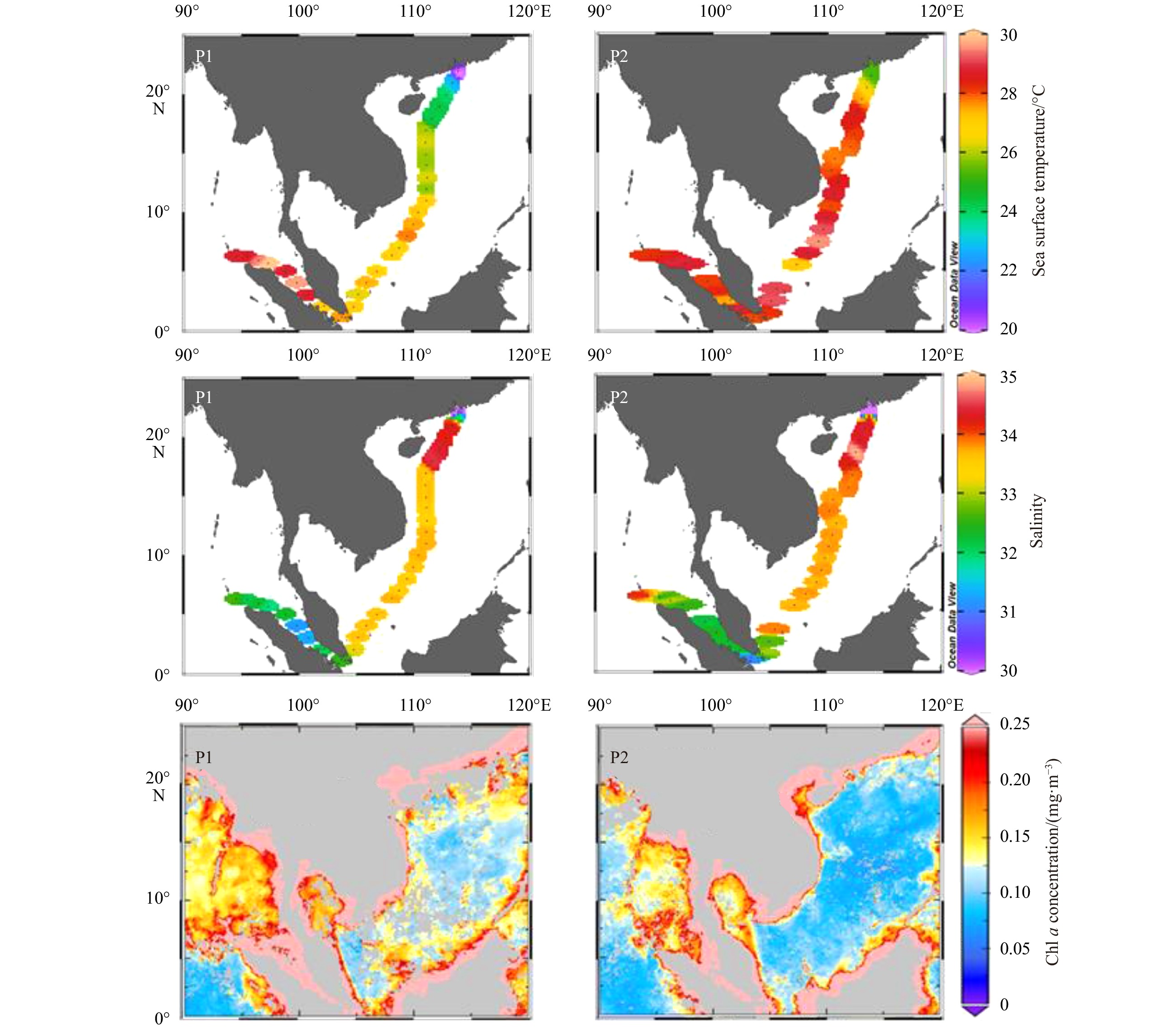
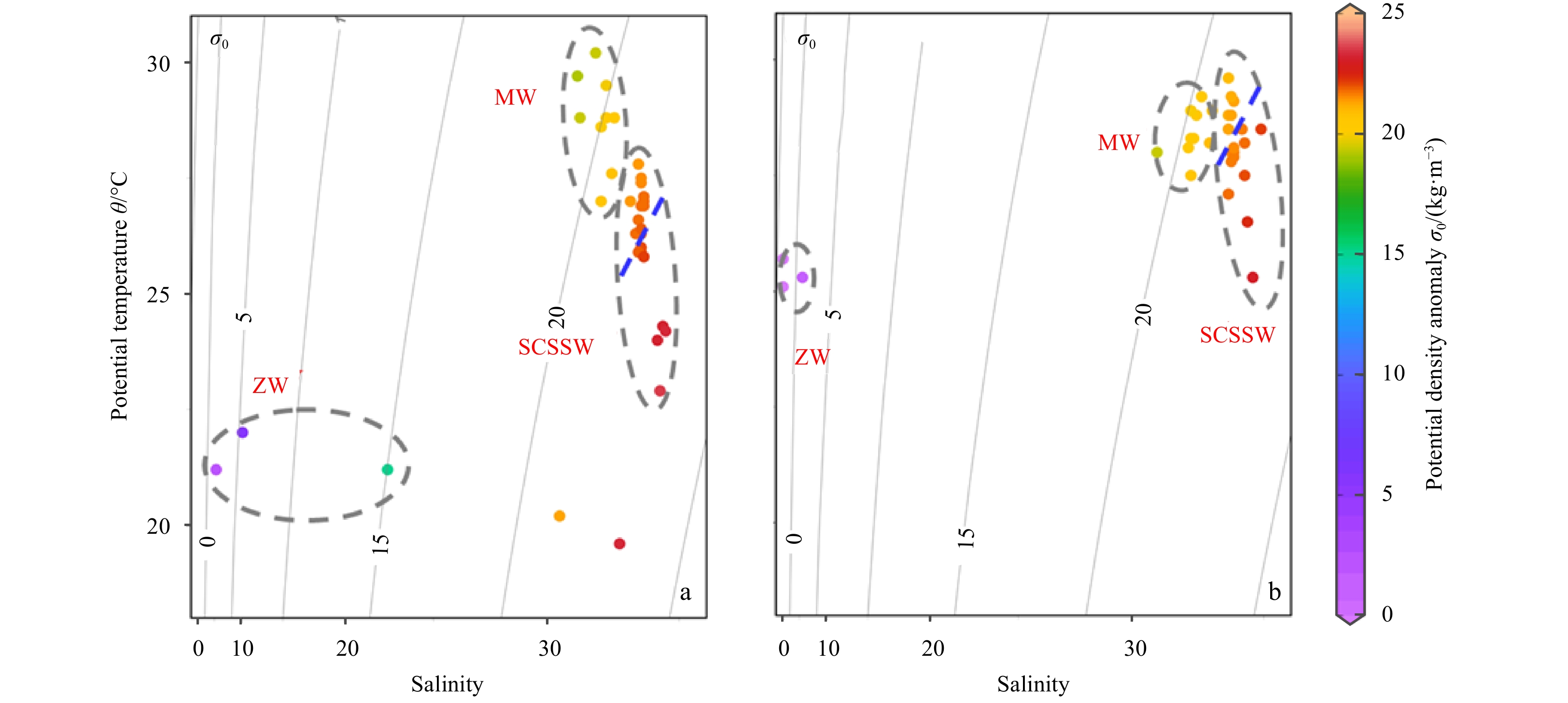
During March 2018 (Fig. 3), water temperature in the ZRE ranged from 19.6°C to 22.0°C. Salinity increased from 0 to 32.8. In the NSCS, water temperature ranged from 22.9°C to 26.3°C (mean of 25.2°C), while the salinity varied between 33.4 and 34.5 (mean of 33.9) and peak value occurred at 18°–22°N, associated with the westward current of the Northwest Luzon Cyclonic Gyre (Fig. 2d). The water temperature in the SSCS elevated (mean of 27.1°C), while the salinity dropped to the range from 32.5 to 33.7 (mean of 33.5). In the MS, surface water temperature ranged from 27.0°C to 30.2°C (mean of 28.9°C) and salinity ranged from 31.2 to 32.3 (mean of 31.9). Remote sensing showed high Chl a concentrations in the ZRE and MS (Fig. 3), over 0.21 mg/m³, while lower values were found in the NSCS (minimum 0.10 mg/m³). During May 2018 (Fig. 3), the water temperature in the ZRE increased to 25.3°C. It also increased in the NSCS and SSCS, while the variation of salinity between March and May 2018 in the SCS was limited. In the MS, the mean temperature was 28.3°C and the salinity was 32.5. The Chl a concentration in the ZRE and MS was still over 0.17 mg/m³, while it significantly declined in the NSCS and SSCS. According to variations in sea surface temperature and salinity, the ZRE, MS, SSCS and NSCS surface water can be clearly identified (Fig. 4). This distribution is in line with the geographical zonation demonstrated in Section 2.1.

Figure  3.  Surface temperature, salinity and Chl a concentration distribution in the ZRE, SCS and MS during March (P1) and May (P2) 2018 (Dataset of Chl a concentration is downloaded from https://giovanni.gsfc.nasa.gov/).

DownLoad: Full-Size Img PowerPoint

Figure  4.  Temperature and salinity diagram during March (a) and May (b) 2018. The major water masses are classified. ZW: Zhujiang River Estuarine Surface Water; MW: Malacca Straits Surface Water; SCSSW: South China Sea Surface Water. The dots at the left of blue dash are southern SCSSW and the right are northern SCSSW; two unclassified dots are the mixing water between ZW and SCSSW.

DownLoad: Full-Size Img PowerPoint

3.2 Dissolved Se species distribution

During March 2018 (Table 1), in the ZRE, Se(IV), Se(VI) and DOSe concentration ranged at 0.14–3.32 nmol/L, 0.53–2.36 nmol/L, 0.01–0.47 nmol/L. In contrast, in the MS, Se(IV) and Se(VI) concentration significantly decreased to 0.05–0.11 nmol/L and 0.21–0.31 nmol/L (one-way ANOVA, p<0.05) (Fig. 5), while DOSe concentration significantly increased to 0.25–0.79 nmol/L (p<0.05). In the NSCS, Se(IV), Se(VI) and DOSe concentration ranged at 0.06–0.10 nmol/L, 0.37–0.44 nmol/L and 0.15–0.66 nmol/L. In the SSCS, Se(IV) (0.05–0.15 nmol/L) and Se(VI) (0.18–0.40 nmol/L) concentrations showed statistically similar variations as the results in the NSCS (p>0.05), while DOSe concentration dropped to 0.01–0.42 nmol/L (p<0.01), except a peak value (0.73 nmol/L). The concentration variability led to the changes of ratios between DOSe, Se(IV) and Se(VI) among different water masses, as outlined in Table 1. In particular, the mean ratio among DOSe, Se(IV) and Se(VI) was 1:5:4 in the ZRE, while it changed to 5:1:4 in the MS and NSCS, 4:1:5 in the SSCS.

Table  1.  Mean concentration and ranges of different Se species in the ZRE, MS, NSCS and SSCS during P1 (March) and P2 (May) 2018

Location	TDSe concentration/(nmol·L–1)			DOSe concentration/(nmol·L–1)			Se(IV) concentration/(nmol·L–1)
	P1	P2		P1	P2		P1	P2
ZRE	2.89	4.42		0.21	0.30		1.51	2.72
	(1.14–6.01)	(3.28–5.64)		(0.01–0.47)	(0.22–0.37)		(0.14–3.32)	(2.00–3.44)
MS	0.91	0.83		0.55	0.44		0.08	0.08
	(0.59–1.11)	(0.57–1.00)		(0.25–0.79)	(0.05–0.66)		(0.05–0.11)	(0.04–0.12)
NSCS	0.93	0.88		0.45	0.42		0.08	0.08
	(0.66–1.12)	(0.71–0.98)		(0.15–0.66)	(0.27–0.54)		(0.06–0.10)	(0.04–0.11)
SSCS	0.68	0.94		0.27	0.52		0.08	0.11
	(0.33–1.18)	(0.75–1.21)		(0.01–0.73)	(0.34–0.77)		(0.05–0.15)	(0.08–0.17)
Location	Se(VI) concentration/(nmol·L–1)			Se(IV)/Se(VI)			DOSe/Se(VI)
	P1	P2		P1	P2		P1	P2
ZRE	1.21	1.50		1.08	1.82		0.27	0.21
	(0.53–2.36)	(1.06–1.82)		(0.27–1.52)	(1.70–1.89)		(0.01–0.90)	(0.01–0.21)
MS	0.28	0.31		0.29	0.28		1.99	1.57
	(0.21–0.31)	(0.25–0.46)		(0.19–0.52)	(0.12–0.41)		(0.94–3.74)	(0.11–2.66)
NSCS	0.40	0.37		0.20	0.22		1.14	1.14
	(0.37–0.44)	(0.34–0.43)		(0.14–0.26)	(0.11–0.30)		(0.34–1.65)	(0.76–1.53)
SSCS	0.32	0.31		0.28	0.36		0.84	1.70
	(0.18–0.40)	(0.21–0.38)		(0.14–0.52)	(0.22–0.81)		(0.06–2.00)	(1.01–2.42)

 | Show Table

DownLoad: CSV

DownLoad: Full-Size Img PowerPoint

5.  Distribution of TDSe, DOSe, Se(IV), Se(VI) concentrations and Se(IV)/Se(VI), DOSe/Se(VI) value in the ZRE, SCS and MS during March (P1) and May (P2) 2018.

DownLoad: Full-Size Img PowerPoint

During May 2018 (Table 1), in the ZRE, concentration ranges of Se(IV), Se(VI) and DOSe were 2.00–3.44 nmol/L, 1.06–1.82 nmol/L and 0.22–0.37 nmol/L, respectively. In the MS, Se(IV) and Se(VI) ranged at 0.04–0.12 nmol/L and 0.25–0.46 nmol/L, respectively, significantly lower than those in the ZRE (p<0.05) (Fig. 5). In contrast, DOSe was 0.05–0.66 nmol/L in the MS, significantly higher than the values in the ZRE (p<0.05). In the NSCS, Se(IV), Se(VI) and DOSe ranged at 0.04–0.11 nmol/L, 0.34–0.43 nmol/L and 0.27–0.54 nmol/L. The seasonal variation was minor for Se species between March and May 2018 (p>0.05) in the ZRE, MS and NSCS. In the SSCS, Se(IV) (0.08–0.17 nmol/L) and Se(VI) (0.21–0.38 nmol/L) also showed similar ranges as concentration ranges found during March 2018, while DOSe significantly enhanced (0.34–0.77 nmol/L) during May 2018 (p<0.01), producing high ratios of DOSe: Se(VI) compared with March 2018.

3.3 Nutrients distributions and the correlations with Se species

Nutrients concentrations in the ZRE, MS, NSCS and SSCS were observed in Table 2. During March 2018, in the ZRE, TDN, DOP, DIP and DSi concentrations were 9.44–713 μmol/L, 0.27–1.97 μmol/L, 0.04–2.85 μmol/L and 2.51–115 μmol/L, respectively, which were significantly higher than the levels in the MS, NSCS and SSCS (p<0.05). DIP and DSi concentrations were statistically similar (p>0.05) among the MS, NSCS, SSCS, while the DOP concentration in the MS ranged 0.14 μmol/L to 0.27 μmol/L and was significantly higher than that in the NSCS and SSCS (p<0.05). During May 2018, nutrients in the ZRE and MS showed insignificantly seasonal variations, while DIP levels in the NSCS and SSCS were significantly declined (p>0.05).

Table  2.  TDN, DOP, DIP and DSi concentrations in the ZRE, MS, NSCS and SSCS during P1 (March) and P2 (May) 2018

Location	TDN concentration/(μmol·L–1)			DOP concentration/(μmol·L–1)			DIP concentration/(μmol·L–1)			DSi concentration/(μmol·L–1)
	P1	P2		P1	P2		P1	P2		P1	P2
ZRE	233	289		0.70	0.18		0.89	1.55		56.6	104
	(9.44–713)	(201–346)		(0.27–1.97)	(0.06–0.30)		(0.04–2.85)	(1.01–1.85)		(2.51–115)	(80.7–117)
MS	4.68	4.72		0.22	0.18		0.09	0.09		1.23	1.40
	(3.97–5.47)	(2.49–7.24)		(0.14–0.27)	(0.08–0.27)		(0.05–0.16)	(0.03–0.20)		(0.72–3.19)	(0.21–5.04)
NSCS	4.12	3.67		0.16	0.18		0.06	0.03		1.25	0.84
	(3.53–4.53)	(3.13–4.83)		(0.12–0.21)	(0.15–0.20)		(0.04–0.08)	(BDL–0.05)		(0.94–1.43)	(0.53–1.28)
SSCS	3.51	4.22		0.10	0.15		0.07	0.05		1.16	1.26
	(1.85–4.65)	(3.46–5.55)		(0.01–0.21)	(0.13–0.18)		(0.03–0.13)	(0.04–0.07)		(0.67–1.59)	(0.66–1.74)

 | Show Table

DownLoad: CSV

In the ZRE (Table S1), Se(IV) and Se(VI) concentration were negatively related with salinity, while positively linked to TDN, DIP and DSi. In the MS (Table S1), DOSe was positively correlated with DOP and concentration of Se(IV) was positively correlated with TDN, DIP and DSi. During March 2018 (Table S2), in the NSCS, Se(IV) showed significant correlations with DIP and DSi. In the SSCS, DOSe had significant correlations with TDN and DOP. During May 2018, the correlations between Se species, especially DOSe, and nutrients were frequently statistically insignificant (Table S2).

4. Discussion

4.1 Spatial variations of Se species

In the ZRE, Se(IV) (mean: 1.92 nmol/L) was the dominant species during the survey (Table 1). Such high concentration was similar to the observation in Yao et al. (2006) (Fig. S1). On a global scale, this phenomenon was contrast to the majority of rivers (>70% of total), especially the rivers in remote areas, where Se(VI) was the dominant chemical species (Cutter, 1989; Cutter and Cutter, 2004). Such contradiction likely results from human disturbance in the watershed. The ZRE is located at a highly populated and industrialized area including metropolises such as Guangzhou, Macao and Hong Kong. Intensive anthropogenic activities, mainly as the industrial practices (e.g., petroleum refining, power production), may release a significant quantity of Se(IV) from their sewage discharge and then increase Se concentrations in the receiving river water (Cutter and Cutter, 2004). The dominance of Se(IV) in the Se inventory was also reported in the Bohai (Se(IV)/Se(VI): 2.74) (Duan et al., 2010) and San Francisco Bay (Se(IV)/Se(VI): 1.20) (Cutter, 1989), where intensive anthropogenic activities were observed along their coastal lines.

In the MS (Fig. 5), Se(IV) and Se(VI) concentrations significantly decreased compared with the ZRE, while DOSe concentration increased (Table 1). Tropical rivers attributed substantial amount of DOSe to estuaries, e.g. DOSe flux of Rajang River and Muludam River in Malaysia ranged 2.78 mol/(km²·a) to 3.55 mol/(km²·a) (Chang et al., 2020). As a region with intensive surface loading (14 rivers in Sumatra and 12 major rivers in Malaysia drain into the MS) (Thia-Eng et al., 2000), the variability of Se inventory is deemed to be responsible for the change of environmental settings in the watershed. In particular, the soil in the South China is frequently to be red clay (Jiang et al., 2018) with low organic matter, while the surrounding coastal areas of the MS are covered with great proportions of peatlands (Jiang et al., 2019) with marked accumulation of terrestrial organic matter (Wu et al., 2019). In Xiamen Jiulong River Estuary, sediment organic selenium has a positive relationship with organic carbon levels (Hu et al., 1996). Coupled with intensive wet precipitation, a significant fraction of organic matter is transported via the surface loading into the receiving coastal seawater (Wit et al., 2015), including a high loading of organic matter associated DOSe, as evidenced by Chang et al. (2020) in several peat-draining rivers in Malaysia. In these peat-draining rivers, dissolved organic carbon (DOC) is frequently enriched, e.g. 2 594 μmol/L DOC concentration in the Siak River (Baum et al., 2007). Considering that Se usually shows a linear relationship with DOC concentration in the tropical zone (Wit et al., 2015), the high proportions of DOSe may be delivered from the surrounding peatlands in the MS. The significant correlation between DOSe and DOP in the MS (Table S1) further reinforced such organic matter transport. In addition, the coastal water in the MS was very turbid due to the surface loading and the resuspension of bottom sediment from tides (Thia-Eng et al., 2000), indicating a potential release of DOSe from sediment sorption-desorption dynamic. Moreover, compared with the ZRE, the dominant anthropogenic activity in the MS surrounding countries is likely to be agriculture (Looi et al., 2013), which accelerates the release of terrestrial organic matter from the soils in the watershed into the coastal seawater. Adding this together, high concentration of DOSe was obtained in the MS. The difference in the Se dominant species between the MS and ZRE, providing a unique ‘‘signature’’ for varies terrestrial inputs and anthropogenic activities.

The terrestrial Se from the surface loading (ZRE and MS surrounding rivers) was rapidly diluted by seawater, as evidenced by the negative correlation between salinity and Se species (Fig. S1). In addition, a significant fraction of Se was rapidly consumed by marine phytoplankton, then transported into biomasses (Cutter and Cutter, 2001). The entire SCS can be classified into NSCS and SSCS based on seasonal variations of surface current circulation (Fig. 2). A similar pattern was identified in the temperature and salinity diagram (Fig. 4). For Se, the Se(IV) concentrations performed low levels and insignificant variation between the NSCS and SSCS (Fig. 5). Such discrepancy might be related with the strong biological assimilation on marine Se(IV). In particular, Se(IV) is strongly impacted by marine phytoplankton activities in the upper layer of oceans (Cutter and Cutter, 1998, 2001), evidenced by a wide range of field observations and laboratory incubations (Baines et al., 2001). As aforementioned, the SCS is enriched with large quantity of phytoplankton species with significant requirement on nutrients and trace elements. Under the strong removal conditions, a constantly low-level Se(IV) among the entire SCS was observed. In addition, the phosphorus concentration in the surface SCS during March 2018 frequently remained the level below 0.21 μmol/L (Fig. S2). Phytoplankton in such oligotrophic oceans may enhance the assimilation of nutrient-like Se, as an alternation (Wang and Dei, 2001). Accordingly, the Se(IV) concentration tended to be similar between the NSCS and SSCS (Fig. 5).

Different with Se(IV) (Fig. 5), Se(VI) and DOSe concentrations significantly decreased in the SSCS compared to that of the NSCS (p<0.05), particularly at the southeast of Vietnam. Indeed, compared with Se(IV), Se(VI) and DOSe are chemically inert for biological assimilation. However, in oligotrophic regions, the absence of allochthonous Se(IV) resulted in the uptake of Se(VI) (Cutter and Bruland, 1984). Between the NSCS and SSCS, a similar concentration of Chl a was obtained during March 2018 (Fig. 3), while water temperature in the SSCS increased to 27.1°C, which likely stimulated the phytoplankton metabolism. Consequently, a consumption of Se(VI), as replacement of Se(IV), was observed in the SSCS. The reduction of DOSe in the SSCS might be more complex since DOSe in seawater is under a dynamic balance. Specifically, it’s widely presumed that phytoplankton can utilize Se(IV) and Se(VI), and released DOSe into the environment through excretion, cell lysis or grazing activity (Besser et al., 1994). The DOSe enrichment is frequently coincided with the high-level primary productivity index, e.g. pigments, bioluminescence and dissolved free amino acids (Cutter and Bruland, 1984). On the other hand, Baines et al. (2001) illustrated that DOSe molecules released from algal cells can be taken up by specific phytoplankton species (e.g. Synechococcus and Dunaliella tertiolecta). This biological consumption rate of DOSe was even similar to that of Se(IV). In the SCS, presence of Synechococcus was reported in the south section but absented in the NSCS during spring (Liu and Chen, 2012). Accordingly, the decline of DOSe in the SSCS may also be resulted from the biological consumption.

4.2 Temporal variations of Se species

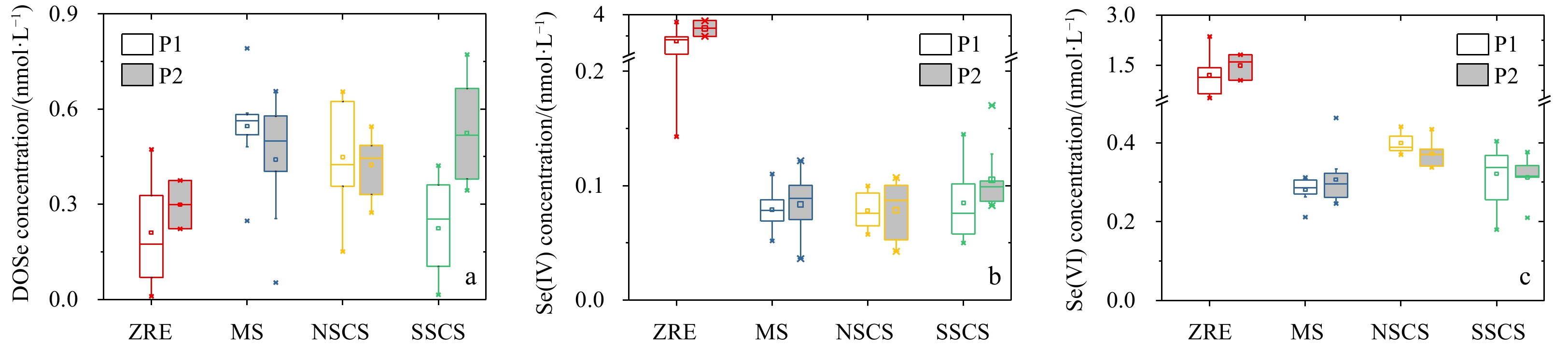
In the ZRE, minor differences in the Se(IV) and Se(VI) concentration between March and May 2018 were observed (Fig. 6). Though the precipitation rate and water temperature might be significantly changed between March and May (Liu et al., 2018), while the Se inventory in the river water was stable, suggesting that soil character and anthropogenic activities might be key factor for the riverine Se concentration. Similarly, in the MS (Fig. 6), the variation of Se inventory between March and May 2018 was also insignificant since both March and May can be identified as the dry season in surrounding coastal zones (Jiang et al., 2019). Together with other nutrient species, the terrestrial Se in both ZRE and MS was also rapidly diluted by seawater and consumed by marine phytoplankton (Fig. S1).

Figure  6.  The DOSe (a), Se(IV) (b) and Se(VI) (c) concentrations in the ZRE, MS, NSCS and SSCS during P1 (March) and P2 (May) 2018. Significant difference of Se(VI) and DOSe concentrations were found between NSCS and SSCS during P1 (p<0.05). DOSe concentration significantly increased in the SSCS during P2 compared to that of P1. The ends of the boxes, the whiskers and the line across each box represent the 25th and 75th percentiles, the 5th and 99th percentiles, and the median, respectively; the square indicates the mean value.

DownLoad: Full-Size Img PowerPoint

In the NSCS, the temporal variation of all Se species was minor (Fig. 6). Interestingly, in the NSCS, the Chl a concentration during May 2018 significantly decrease (Fig. 3), indicating a slow biological consumption and subsequently Se accumulation in the surface seawater. On the other hand, the enhanced stratification in the upper layer driven by temperature increased during May (Zeng et al., 2016), which decreased the vertical mixing between upper water and deep Se-enriched water. Accordingly, the supply of Se from the deep water to the surface reduced, leading to minor enrichment in the surface water though consumption rate was assumed to be significantly decreased. Different with the NSCS, a significant increase of DOSe was observed in the SSCS (Fig. 6a). Two reasons might be important. Firstly, in the SSCS, the surface current reversed during May and the Southeast Vietnam Offshore Current appeared (Fig. 2e), leading to an enhanced input of terrestrial Se, especially DOSe, from tropical coasts to the SSCS. The current may also introduce a fraction of coastal phytoplankton to the SSCS. Compared with the coastal environment, the SSCS was oligotrophic during May (Fig. S2), which could not sustain a high primary production. The intruded phytoplankton from the Vietnam coast (Wang and Tang, 2014) might be decayed in such seawater environment and released Se from cellular biomass via catabolic transformations (Ivanenko, 2018), increasing DOSe concentrations in the SSCS. In addition, during May 2018, Chl a concentration in the SSCS markedly decreased, indicating a decline of biomass for DOSe consumers (Synechococcus). Accordingly, the DOSe assimilation rate decreased. The balance between DOSe consumption and accumulation changed, enhancing the DOSe concentration in the SSCS.

4.3 Se species in the surface waters at a global view

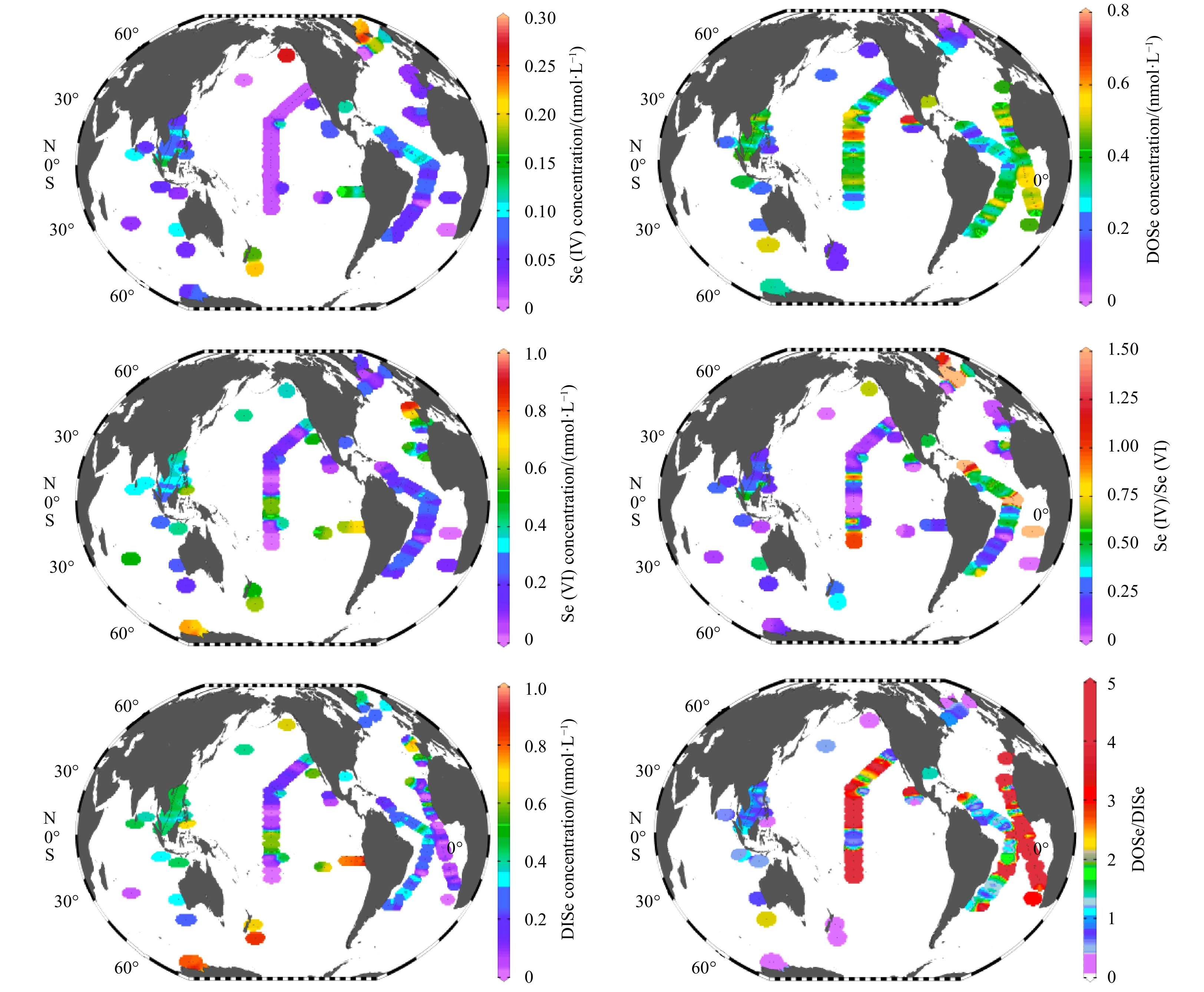
Se compositions obtained from the SCS would be reviewed at a global view via comparing with other oceanic survey results (Fig. 7). In the SCS, Se(IV) (0.04–0.17 nmol/L) and Se(VI) (0.18–0.44 nmol/L) values were obtained and took up 9% and 41% of TDSe (Fig. 5). In other tropical oceans, a similar range was observed. For instance, in the tropical Pacific Ocean and Atlantic Oceans (Se(IV): <0.15 nmol/L, Se(VI): 0.02–0.59 nmol/L) (Cutter and Bruland, 1984; Cutter and Cutter, 1998, 2001). The elevated Se(VI) in the tropical Pacific Ocean was associated with local equatorial upwelling, introducing Se(VI) enriched deep water into ocean surface, as well as east coastal of Atlantic Ocean (0°–30°N). DOSe concentration (0.01–0.77 nmol/L) in the SCS (Fig. 5) was also close to that in the tropical Pacific Ocean (0.06–0.75 nmol/L) (Aono et al., 1991; Cutter and Bruland, 1984; Nakaguchi et al., 2004; Rue et al., 1997; Takayanagi and Wong, 1985), the tropical Atlantic Ocean (<0.45 nmol/L) (Cutter and Cutter, 1995, 2001) and Indian Ocean (0.24 nmol/L) (Hattori et al., 2001). Such low-level Se suggests the strong biological assimilation in tropical oceans. In addition, in the Se inventory, DOSe accounted for the dominant fraction of the TDSe (DOSe/TDSe: 0.48) in the SCS (Fig. 5), consistent with Se species fractions in the tropical Pacific Ocean (DOSe/TDSe: 0.66), tropical Atlantic Ocean (DOSe/TDSe: 0.50) and Indian Ocean (DOSe/TDSe: 0.47) surface water, as outlined in Fig. 7. As aforementioned, DOSe can be produced from phytoplankton metabolization (Ivanenko, 2018), as the product from cell decay or exudation (Araie and Shiraiwa, 2016). In the tropical oceans, including SCS, the dominant phytoplankton species was frequently to be Prochlorococcus (Flombaum et al., 2013). This wide distribution of Prochlorococcus with relatively high biomass likely produces the similar enrichment of DOSe in the marine environment.

Figure  7.  Concentrations of Se(IV), Se(VI), DISe, DOSe, and values of Se(IV)/Se(VI) and DOSe/DISe surface seawater in global oceans (Dataset of the ZRE, SCS and MS are from this study. Others are from Aono et al., 1991; Cutter and Bruland, 1984; Cutter and Cutter, 1995, 1998, 2001; Harrori et al., 2001; Measures et al., 1983; 1980; Measures and Burton, 1980; Nakaguchi et al., 2004; Rue et al., 1997; Takayanagi and Wong, 1985; Wambaugh, 2017; Xia et al., 1996).

DownLoad: Full-Size Img PowerPoint

Se species varied from the tropical ocean to the high-latitude ocean (Fig. 7), changing from the DOSe-dominance to the DISe-dominance. In particular, in the high-latitude ocean (e.g. the North and South Pacific Ocean), DOSe/DISe was below 1. In the high-latitude of Northern Hemisphere, Se(IV) was the main species with Se(IV)/Se(VI) above 1. While in the Antarctic Ocean, the proportion of Se(VI) in the seawater increased to 55% of TDSe (Xia et al., 1996) and Se(VI) became the major species. In a word, the dominate Se species in high-latitude ocean was Se(IV) (Northern Hemisphere) and Se(VI) (Southern Hemisphere), while changed to DOSe in the tropical oceans. Previous investigations reported that high inorganic Se concentration (Se(IV) and Se(VI)) in high-latitude oceans may be associated with the slow growth of phytoplankton in mesotrophic regions, reducing the biological demand for Se (Cutter and Cutter, 1998). Low concentration of biogenic particles and slow degradation rate play a negative role on the DOSe accumulation (Cutter and Cutter, 1998). Furthermore, the dominant phytoplankton varied in different latitudinal oligotrophic oceans (Flombaum et al., 2013). In the high-latitude ocean, diatoms, a species with biological requirement on Se (Harrison et al., 1988), are frequently to be dominant species, especially along the coasts. This distribution may lead to different Se biogeochemical cycle compared to the tropical ocean (Wake et al., 2012). In addition, Synechococcus-like cyanobacteria, a species utilizing DOSe, is dominated in colder subtropical regions and in the equatorial upwellings (Flombaum et al., 2013; De Boissieu et al., 2014), which explains the relatively low DOSe value in the northeastern of tropical Atlantic Ocean (0°–20°N) (Cutter and Cutter, 1995). Accordingly, the variability of phytoplankton species in global oceans might deeply change the distribution of Se species. During laboratory incubations, Diatoms, Dinophyceae, Prasinophyceae, Cyanobacteria and Chlorophyceae incorporated 42%–53%, 42%, 30%, 32% and 4% of the dissolved Se using radiolabeled selenite (Baines et al., 2001), suggesting variable assimilation efficiency of different phytoplankton communities to Se species (Baines and Fisher, 2001; Harrison et al., 1988). Haptophytes and diatoms have a Se-requirement for their growth, while the green algae require Se to synthesize selenoproteins instead of growth (Araie and Shiraiwa, 2016). Though previous investigation reported few marine phytoplankton (Chaetoceros pelagica, Sekeletonema costatum, Thalassiosira rotula) uptake Se species, it’s still ambiguous about the detailed processes and functions of Se in phytoplankton metabolism (Harrison et al., 1988). Further investigation on the impact of marine phytoplankton behavior on Se species should be carried out in the future. To conclude, the dominant phytoplankton performed a profound role in surface Se species distributions and behaviors in different oceanic regimes.

5. Conclusion

DOSe, Se(IV) and Se(VI) concentrations in surface water were investigated in the ZRE, MS and the SCS during March (P1) and May (P2). The results showed that Se(IV) was the predominant species in the ZRE, while DOSe was the major fraction in the MS, which was associated with the varied terrestrial inputs and anthropogenic activities. In the NSCS and SSCS, DOSe and Se(VI) were relatively enriched in the seawater compared to Se(IV). The low-level Se(IV) in surface water of the entire SCS resulted from the preferential uptake Se(IV) by marine phytoplankton in oligotrophic oceans. During March 2018, DOSe in the SSCS was significantly lower than that in the NSCS, due to the intense consuming by primary producers (e.g. Synechococcus) in the SSCS. During May 2018, the temporal variation of Se concentration, including Se(VI), Se(IV) and DOSe in the NSCS was minor. In contrast, the DOSe concentration significantly increased in the SSCS, which may be the result of the Southeast Vietnam Offshore Current that introduced substantial land-derived DOSe from tropical coasts. In addition, the current may also transport coastal phytoplankton. The cell decay of these phytoplankton in the SSCS likely added DOSe in the seawater. Together with decreases of Chl a concentration (weak assimilation), the relative DOSe enrichment was observed. On a global scale, the enrichment of DOSe found in the SCS was also observed in other tropical oceans, while in high-latitude oceans, Se(IV) and Se(VI) became the major faction in seawater, which may be the result of changing predominate phytoplankton species (diatom) and decreased biological assimilation. Further investigation on the effect of Se speciation for varied marine phytoplankton species should be conducted in the future to improve the knowledge on the biological role of Se in different oceanic regimes.

Acknowledgements

We appreciate the sampling and logistic support from the captain and crews of the R/V Shiyan III and South China Sea Institute of Oceanology (Chinese Academy of Sciences). We thank our colleagues, Yixue Zhang, Shuo Jiang, Xiaohui Zhang, Yao Wang, and Yuxi Ma, from East China Normal University for the assistance in collecting samples and conducting analyses. Anonymous reviewers and editor are especially acknowledged for their constructive suggestions, which greatly improved the manuscript.