Three-dimensional structure of an observed cyclonic mesoscale eddy in the Northwest Pacific and its assimilation experiment

1. Introduction

Mesoscale eddies are widespread throughout the ocean, and are the most energetic forms of motion prevailing in the ocean (Wang et al., 2003), responsible for approximately 90% of the kinetic energy in the ocean (Ferrari and Wunsch, 2009). Additionally, mesoscale eddies play important roles in the distribution of marine material, water mass, and energy exchange between the ocean and atmosphere (Zhang et al., 2014; Ma et al., 2016).

At present, altimeter sea level anomaly (SLA) data are widely used to identify and track mesoscale eddies. Previous studies mainly used statistical algorithms to analyze the number, radius, amplitude, lifetime, and geographical distribution of mesoscale eddies (Wang et al., 2003; Chelton et al., 2011). However, satellite altimeter data can only reflect the characteristics of the sea surface, and the vertical structure of the eddies cannot be presented well. The in situ measurements combined with altimeter observation is an effective method to study the three-dimensional structure of eddies. Zhang et al. (2016) analyzed the three-dimensional structure, generation, and dissipation mechanisms of a pair of cold and warm eddies by two bottom-anchored subsurface mooring arrays with altimeter observation. Zhang et al. (2018) combined Argo (Array for Real-time Geostrophic Oceanography) observations and SLA to reconstruct a three-dimensional structure of an eddy in the Luzon Strait with a composite method and analyzed its impact on the marine environment. Shu et al. (2019) conducted regional observations to study the three-dimensional structure and temporal evolution of an anticyclonic mesoscale eddy with 12 gliders and 62 expendable probes in the northern South China Sea during the summer of 2017. Dai et al. (2020) used a high spatial resolution Argo array with 17 rapid sampling Argo floats to reconstruct the three-dimensional structure of an anticyclonic mesoscale eddy in the Northwest Pacific and analyze its heat/salt transport.

However, the observation data remain too sparse in the Pacific Ocean for research (Liu et al., 2018a). Therefore, numerical models are also powerful tools for scholars to study mesoscale eddies. Rubio et al. (2009) investigated the origin and dynamics of “Catalan eddies” using a numerical circulation model of the northwest Mediterranean at 3 km resolution, and the hydrology and dynamics of the structures were characterized compared with the observations in the Catalan Sea. Lin et al. (2013) used the Regional Ocean Modeling System (ROMS) model with (1/12)° resolution to reproduce the generation and dissipation of a Dongsha cold eddy from the September to October of 2000, and the eddy’s surface characteristics and three-dimensional structure were also analyzed. Wang and Gan (2014) discussed the three-dimensional structure of the eddy on the west side of Luzon based on the Princeton Ocean Model (POM) with a resolution of 10–30 km. He et al. (2015) used the MIT General Circulation Model (MITgcm) with a resolution of (1/6)° to describe the three-dimensional structure and spatiotemporal variation characteristics of the Luzon cold eddies in the northern South China Sea, and noted that the cold eddies in upper and deeper layers were based on different generation mechanisms.

Although a few high-resolution models can simulate mesoscale eddies independently, the generation and motion of the eddies are difficult to correspond with the observation in time due to the lack of data assimilation. Data assimilation can help estimate the state of ocean circulation better (He et al., 2008; Liu et al., 2018b, 2020; Shu et al., 2011), which is helpful for more detailed research on the three-dimensional structure and other eddy characteristics. Gao et al. (2008) used the three-dimensional variational data assimilation system combined with the POM model to perform mesoscale eddy assimilation simulation experiments in the Northwest Pacific Ocean. The results show that the simulation results of assimilation with sea surface height anomaly data are far better than those without assimilation. Ferron (2011) used a (1/3)° eddy-permitting model combined with a 4D-variational method to estimate the mesoscale eddy from altimeter observations in the North Atlantic. Comparing the observations (Argo floats and CTD data) along the OVIDE cruise in 2002, the ocean state after assimilation show an obvious improvement compared with those without assimilation. Based on the data assimilation and the Hybrid Coordinate Ocean Model (HYCOM) with (1/12)° resolution, Xu (2012) reproduced the generation and development of two anticyclones in the northern South China Sea in the winter of 2003 and 2004. Zhao et al. (2017) used the ensemble optimal interpolation method to assimilate along track sea level anomaly data into a (1/30)° high-resolution ocean model, and simulated a pair of cold and warm eddies in the sea to the southwest of Taiwan Island with asymmetric velocity structure and vertical-tilting eddy structure.

Although the research on mesoscale eddies is developing, the three-dimensional structure of global ocean mesoscale eddies is still under exploration (Zhang et al., 2013; Dong et al., 2017). At present, the three-dimensional structure of mesoscale eddies in the Northwest Pacific is mostly based on composite analysis, which only reflects the average state of the characteristics. Due to the limitation of the measuring method, specific observation on individual mesoscale eddy is still rare, especially on their three-dimensional structure. In addition, most of the current studies on the assimilation of mesoscale eddies usually assimilated sea surface height (SSH), sea surface temperature (SST) and Argo profiles into the model. Due to the limitation of observation, few studies assimilated the in situ measurement by oceanographic survey, and used the assimilation results to study the three-dimensional structure of mesoscale eddies. In this study, a cyclonic eddy captured during an oceanographic cruise in November 2019 in the Northwest Pacific Ocean was investigated. This study used the high resolution ROMS model at (1/20)° resolution with the four-dimensional variational data assimilation (4DVAR) system to reproduce this eddy, by assimilating SSH, SST, and in situ measurement by survey into the system. Combined with the observation and assimilation results, it is helpful for us to study the three-dimensional structure and other characteristics of this cyclonic eddy. This study is organized as follows. Section 2 describes the main data and method in this study. Section 3 analyzes the surface properties and three-dimensional structure of eddy from observations. Section 4 describes the four-dimensional variational assimilation system in detail and the assimilation effect is verified. Section 5 analyzes the three-dimensional structure of eddy from the assimilation results. Based on the high-resolution assimilation output, the diagnosis of vertical velocity and the nature of water mass within the eddy are also discussed in this section. Finally, Section 6 summarizes the conclusions.

2. Data source and methodology

2.1 Satellite altimeter data

The satellite altimeter data used to identify and track cyclonic eddy in this study come from the Copernicus Marine Environment Monitoring Service (CMEMS, https://marine.copernicus.eu/). The product’s name is the Global Ocean Gridded L4 Sea Surface Heights and Derived Variables Reprocessed Product, which is estimated by optimal interpolation, merging the measurement from the different altimeter missions available. The resolution of this product is 0.25°×0.25° with a time interval of one day. Furthermore, it processes data from all altimeter missions: Jason-3, Sentinel-3A, HY-2A, and others.

2.2 CARS2009 climatology data

The CSIRO Atlas of Regional Sea 2009 (CARS2009, http://www.marine.csiro.au/-dunn/cars2009/) climatology data in this study are compared with the thermohaline profile to reflect the temperature and salinity anomalies of the mesoscale eddy. The climatology data are provided by CARS2009. CARS2009 covers the global oceans on a 0.5°×0.5° grid, including temperature and salinity fields. It is derived from the quality-controlled dataset of all available historical observation data, including vessel instrument profiles and autonomous profiling buoys. As data availability has enormously improved, the CARS mean values are inevitably biased towards the real ocean state. The formula for calculating the climate state of CARS2009 on a certain day is (Ni, 2014):

where var is the three-dimensional climatology temperature (salinity) data; mean, an_cos, an_sin, sa_cos, and sa_sin are global three-dimensional fields provided by CARS2009; and t represents the day of the year.

2.3 Temperature, salinity, and current data from in situ measurements

The mesoscale eddy was measured during a vessel-based underway survey. Seven zonal sections and one meridional section within the range of the mesoscale eddy were designed to investigate its structure. The distribution of observation stations is shown in Fig. 1b. The temperature and salinity data are measured by the MVP 300 measurement system, which obtain the temperature and salinity profiles every half an hour. The horizontal resolution depends on the sailing speed. During the survey period, the ship mainly moved at two speeds. When the speed is 11 kn, the horizontal resolution is about 10 km, and when the speed is 7 kn, the resolution is about 6.5 km. The temperature and salinity data are continuously measured in the vertical direction by MVP 300, the measured range is 10–550 m, and the vertical resolution is 1 m. The time resolution of the current data measured by Acoustic Doppler Current Profiler (ADCP) is 5 min, and the vertical resolution is 16 m. The measurement range is from the sea surface to the depth of 700 m. In order to ensure the quality of the data measured by ADCP, the time continuity of the data is checked. And the current velocity data measured when the speed is too low are removed.

Figure  1.  Eddy trajectory during its life cycle (a) and the distribution of observation stations (b). The survey was conducted from November 13 to 15, 2019 during the short red line segment. In a, the black thick line represents the trajectory of eddy center and black thin line represents the eddy edge on November 13, 2019, while the eddy center is at 26.28°N, 137.54°E. In b, the black dots represent the observation stations. The yellow dot is the center of the eddy, and the black line represents the eddy edge.

DownLoad: Full-Size Img PowerPoint

2.4 Other datasets

Reanalysis data of the HYCOM, SST data and ERA5 reanalysis data are used for realistic simulation. The reanalysis dataset of HYCOM (https://www.hycom.org/) is a global daily product with a spatial resolution of (1/12)°, and it assimilates multiple kinds of observations including SLA, SST, temperature and salinity profiles observed by Argo and moored buoys.

SST is from CMEMS (https://marine.copernicus.eu/). The product’s name is SST_GLO_SST_L4_NRT_OBSERVATIONS_010_005, whose resolution is 0.25°×0.25° with a time interval of one day. It is a product that the Met Office uses GHRSST Multi-Product Ensemble (GMPE) system to take inputs from various analysis production centers on a routine basis and produces ensemble products at 0.25°×0.25° horizontal resolution.

ERA5 is the fifth generation European Centre for Medium-Range Weather Forecasts (ECMWF) atmospheric reanalysis of the global climate (https://www.ecmwf.int/en/forecasts/datasets/reanalysis-datasets/era5). ERA5 has a horizontal resolution of 0.25°×0.25° in the atmosphere and a horizontal resolution 0.5°×0.5° in the ocean wave. It was produced by 4D-variational data assimilation in Cycle 41r2 of ECMWF’s integrated forecast system.

2.5 Eddy identification and tracking method

The eddy identification method is mainly based on the contours of SSH, referring to the method proposed by Chelton et al. (2011) and Ni (2014). The SLA contour-based method has great advantages over the Okubo Weiss method in terms of precision and accuracy (Souza et al., 2011). The identification process includes the four steps: (1) derive contours every 0.5 cm from the SLA field; (2) consider the geometric center of the innermost closed contour line as the eddy center; (3) the eddy edge is the closed contour of the outermost circle containing the unique eddy center; (4) the type of eddy can be judged by comparing the SLA values of the eddy center and edge. When the SLA value of the eddy center is greater than that of the eddy edge, it is a warm eddy; otherwise it is a cold eddy.

The similarity method is used to track the mesoscale eddy (Chaigneau et al., 2008; Dai et al., 2020). The similarity method is based on a dimensionless similar parameter distance ${S_{{{\rm{e}}_1},\;{{\rm{e}}_2}}} $, consisting of distance difference ΔD, radius difference ΔR, eddy kinetic energy difference ΔEKE, and vorticity difference Δζ.

The standard distance D₀, radius R₀, eddy kinetic energy EKE₀ and vorticity ζ₀ are 100 km, 100 km, 100 cm²/s² and 10^–6 s⁻¹, respectively. The algorithm considers that the eddy pair (e₁, e₂) with the smallest ${S_{{{\rm{e}}_1},\;{{\rm{e}}_2}}} $ values is the target eddy. This method can avoid trajectory interruption (Chen et al., 2011), and significantly decreases the number of “false” identified eddies (Chaigneau et al., 2008).

2.6 Divand method

Divand method (Barth et al., 2014; Troupin et al., 2012) is a multidimensional variational interpolation method, which is a practical application of the variational inverse method. This method interpolates the observation value into the target grid by minimum cost function, and obtains a continuous field close to the observation. The cost function is:

where J is the cost function, and N_d is the number of data point. d_j represents the measured value at (x_j, y_j), u_j is the weight, and $\left\| \varphi \right\|$ is expressed as:

where D represents the domain of interest, $ \nabla \nabla \varphi$: $ \nabla \nabla \varphi$ represents the smoothness constraint term, and its formula is as follows:

In Eq. (5), α₀ represents the continuous field’s coefficient, α₁ represents the gradient and α₂ represents the rate of variation. Based on topography and topology, the method can naturally decouple disconnected regions. Water masses that are not contiguous in the ocean usually have different physical properties, so this method is very practical in the ocean. However, for optimal interpolation method, it is difficult to separate and decouple the land and water masses while maintaining a smooth spatial field in the ocean (Barth et al., 2014). In addition, Divand method is a good choice for the interpolation of scatter data.

3. Three-dimensional structure of the eddy from observation

3.1 Trajectory and surface properties

The satellite altimeter data from CMEMS were used to track the target eddy by the method detailed in Section 2, and its trajectory is shown in Fig. 1a. The cyclonic eddy was generated in 24.6°N, 139.6°E on September 25, 2019, and died out in 28.6°N, 131.6°E on February 28, 2020, lasting for 157 d. During its life cycle, it generally moved northwest approximately 1 520.5 km. The average propagation velocity was approximately 0.11 m/s.

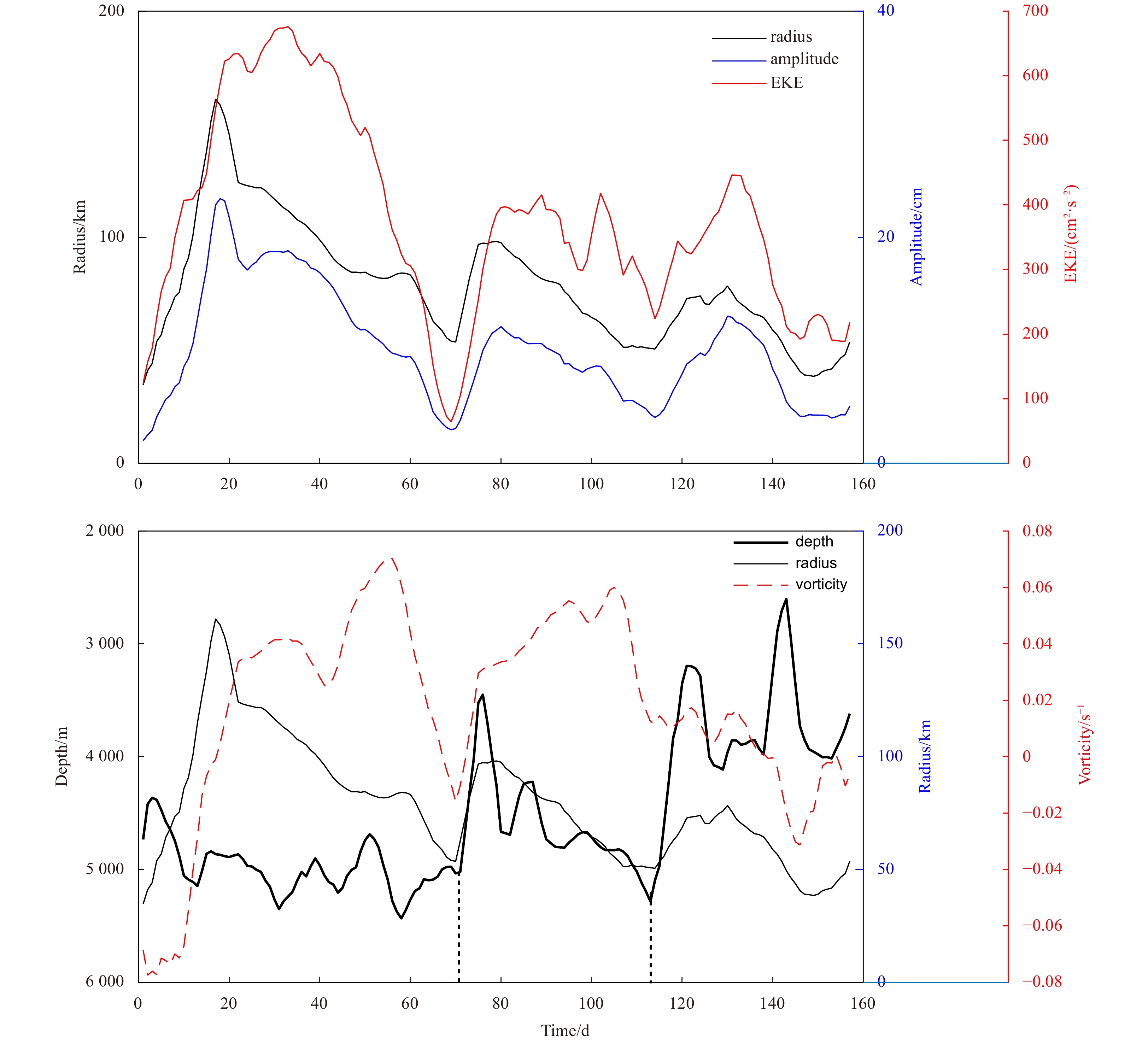
In this study, the radius of the eddy is defined as the radius of a circle of equal area: $R = \sqrt {\dfrac{S}{\pi }} $, S is the area of the eddy. The amplitude A is defined as the difference between the SLA of the eddy center and the eddy edge: A=SLA_center–SLA_edge. The eddy kinetic energy (EKE) is defined as the average value of the eddy kinetic energy: ${\rm{EKE}} = \dfrac{{{u^2} + {v^2}}}{2}$. Figure 2 shows the variation of eddy’s radius, amplitude, vorticity, eddy kinetic energy and depth during its life cycle. The average radius of the eddy during its life cycle is 78.8 km. It can be found that the radius, vorticity, amplitude and eddy kinetic energy have similar trends and these parameters are positively correlated. The radius of the cold eddy increases rapidly after its generation, and then followed by two significant fluctuations, corresponding to two topographic changes (the black dotted lines). The fluctuations reflect eddy’s adjustment to the topography (Kamenkovich et al., 1996; Beismann et al., 1999). Kamenkovich et al. (1996) used a two-layer primitive equation model to carry out numerical experiments on the interaction between eddy and topography. They found that the eddy crossing the ridge would show an intensification before the eddy center encounters the ridge. The specific manifestation is the increase in SSH and the deepening of the thermocline. This phenomenon can be observed in the actual ocean by altimeter data. Beismann et al. (1999) found in numerical experiments that when the eddy approaches the ridge, the intensity of the eddy increases due to the deflection of the layer interface. In this study, the eddy’s radius begins to increase rapidly when the eddy center approaches the ridge.

Figure  2.  The variation of topographic depth, radius, vorticity, amplitude and eddy kinetic energy of the cold eddy during the eddy’s life cycle.

DownLoad: Full-Size Img PowerPoint

3.2 Three-dimensional structure analysis from observation

The three-dimensional structure plays an important role in understanding the characteristics of mesoscale eddies. In this section, three-dimensional structure of an individual cyclonic mesoscale eddy is illustrated in detail by the vertical section and the horizontal slice of temperature, salinity and velocity.

3.2.1   Temperature and salinity field structure

The profile of the temperature and salinity is conducted by analyzing the zonal section that crosses the center of eddy. Figures 3a and c show the vertical temperature and salinity profile, and Figs 3b and d represent the vertical temperature and salinity anomaly. Since the investigation only reached the depth of 550 m, this study mainly focused on the structure from the sea surface to 550 m. The anomaly value is derived by subtracting the CARS2009 climatology data from the observation.

Figure  3.  Observed vertical temperature section (a), temperature anomaly (b), salinity section (c), and salinity anomaly (d) of the cold eddy in the zonal direction. The grey lines represent the potential density, and the numbers are the values of potential density.

DownLoad: Full-Size Img PowerPoint

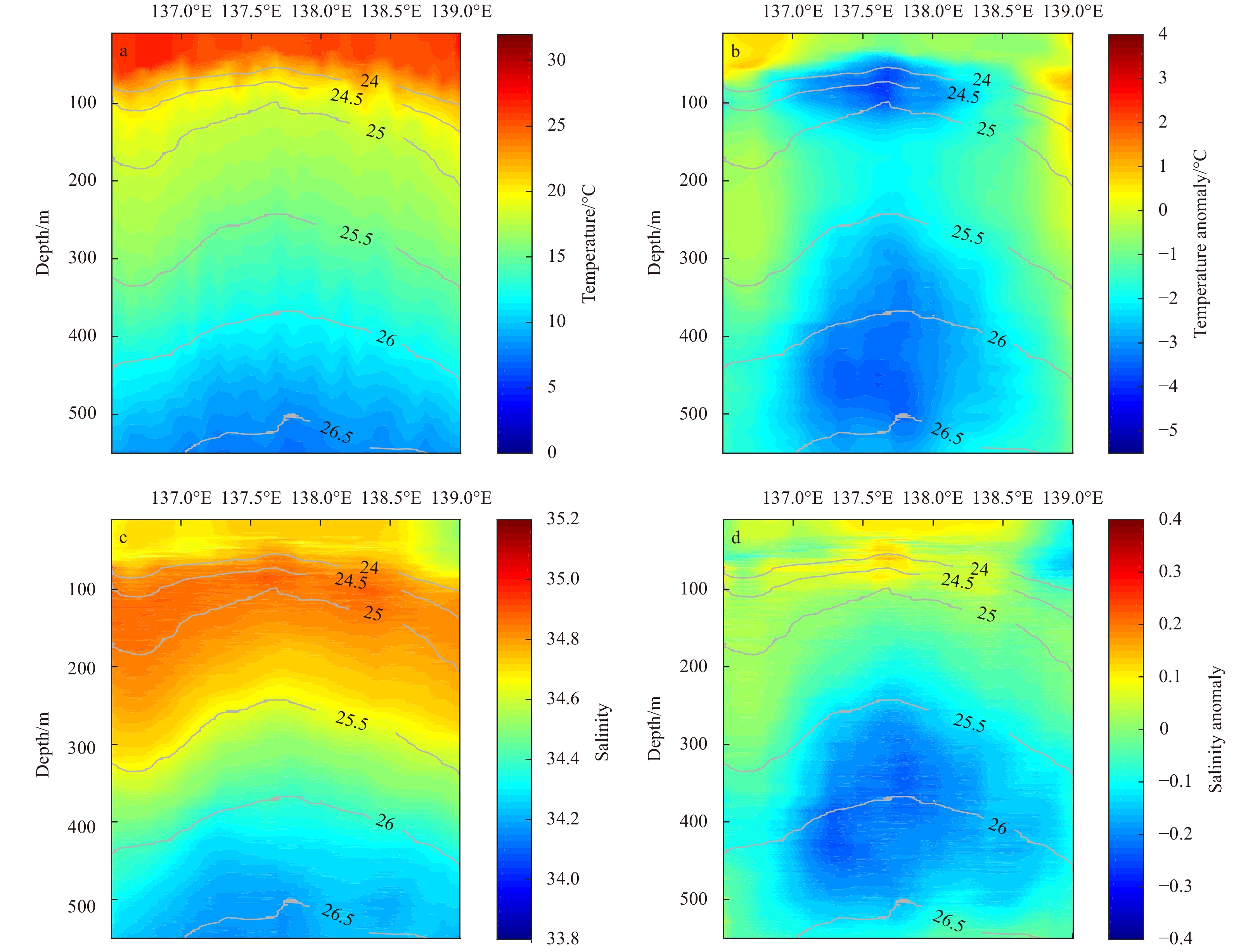
The isotherms in Fig. 3a consistently exhibited enhanced upward bending. The temperature anomaly of upper and deeper layer in Fig. 3b both have significantly lower temperature than the surroundings, and show that the cold eddy has a dual-core vertical structure. The core in the upper layer of the eddy is at 50–150 m and in the deeper layer is 300–550 m. The result verifies the conclusion of Yang et al. (2013) obtained from the composite eddy that one core is above 200 m, and the other is between 300 m and 700 m in the Northwest Pacific. In this study, the temperature anomaly values of the two cores are close to each other, and the average anomaly is approximately −3.5°C. The dual-core structure is related to the North Pacific Subtropical Mode Water (STMW) with low potential vorticity in the main thermocline (Yang et al., 2013; Dong et al., 2017), which can be interpreted as the interaction between the eddy and STMW. STMW divides the main thermocline into upper (>19°C, <200 m) and deeper (8–15°C, 350–700 m) layers. The upwelling of the cold eddy will make the thermocline convex, and the lifting effect of the eddy on the upper thermocline is stronger than that on the deeper thermocline (Ni, 2014). Therefore, the upper and deeper thermocline are separated more, which makes the upper and deeper cores more obvious.

The isohalines in Fig. 3c had similar characteristics to the isotherms. The isohalines also trended upwards, and became more pronounced in the subsurface. In Fig. 3d, the salinity anomaly exhibited one clear eddy core structure, with a negative anomaly approximately −0.3 at 250–500 m. Salinity at 10–100 m had a positive anomaly approximately 0.1. The negative anomaly is due to the upward movement of water caused by the cyclonic eddy, which makes the low-salt North Pacific Intermediate Water (NPIW) rise upwards and then reduces the salinity of the water above it. And then the subsurface high-salt North Pacific Tropical Water (NPTW) was also lifted upwards, resulting in positive salinity anomalies on the surface.

The horizontal slices of the cold eddy temperature and salinity anomaly at some specific depth layers are shown in Fig. 4. The depths of the slices are 10 m, 100 m, 200 m, 300 m, 400 m and 500 m. Divand variational interpolation method (Barth et al., 2014) is used to interpolate the temperature and salinity data of each layer. The interpolation field subtracts the CARS009 climatology data to obtain the slice of the anomaly value.

Figure  4.  The slice map of temperature (a) and salinity (b) anomaly with depths of 10 m, 100 m, 200 m, 300 m, 400 m and 500 m.

DownLoad: Full-Size Img PowerPoint

The isotherm in Fig. 4a remained a closed circulation structure from 100 m to 500 m, indicating a stable eddy structure. The negative temperature anomaly at 100 m was obviously larger than that of 10 m and 200 m, reaching about −3.5°C; therefore, it is obvious that there exists a cold core at approximately 100 m. Another cold core was reflected by the negative temperature anomaly between 300 m and 500 m, with its temperature anomaly value reaching approximately −3.5°C. Therefore, a clear dual-core vertical structure is also clearly reflected in the temperature anomaly slice map.

The salinity anomaly slice of the cold eddy at the same depth is shown in Fig. 4b. A positive salinity anomaly about 0.1 was clearly observed on the surface, and a significant negative anomaly appeared at 300–500 m, which is consistent with the previous analysis of the vertical salinity profile. In the vertical direction, the positive salinity anomaly gradually decreased from 10 m to 200 m, and the negative anomaly first decreased and then increased between 200 m and 400 m. The absolute value of the maximum anomaly appeared at the 400 m layer, at approximately −0.3.

3.2.2   Three-dimensional structure of velocity

The three-dimensional velocity structure is reflected by geostrophic current anomaly and the velocity slice at some specific depths. Figures 5a and b show the geostrophic current anomaly in the zonal and meridional directions. The geostrophic current anomaly V′ (u′, v′) was derived from the dynamic height anomaly H′. The dynamic height H is computed as follows:

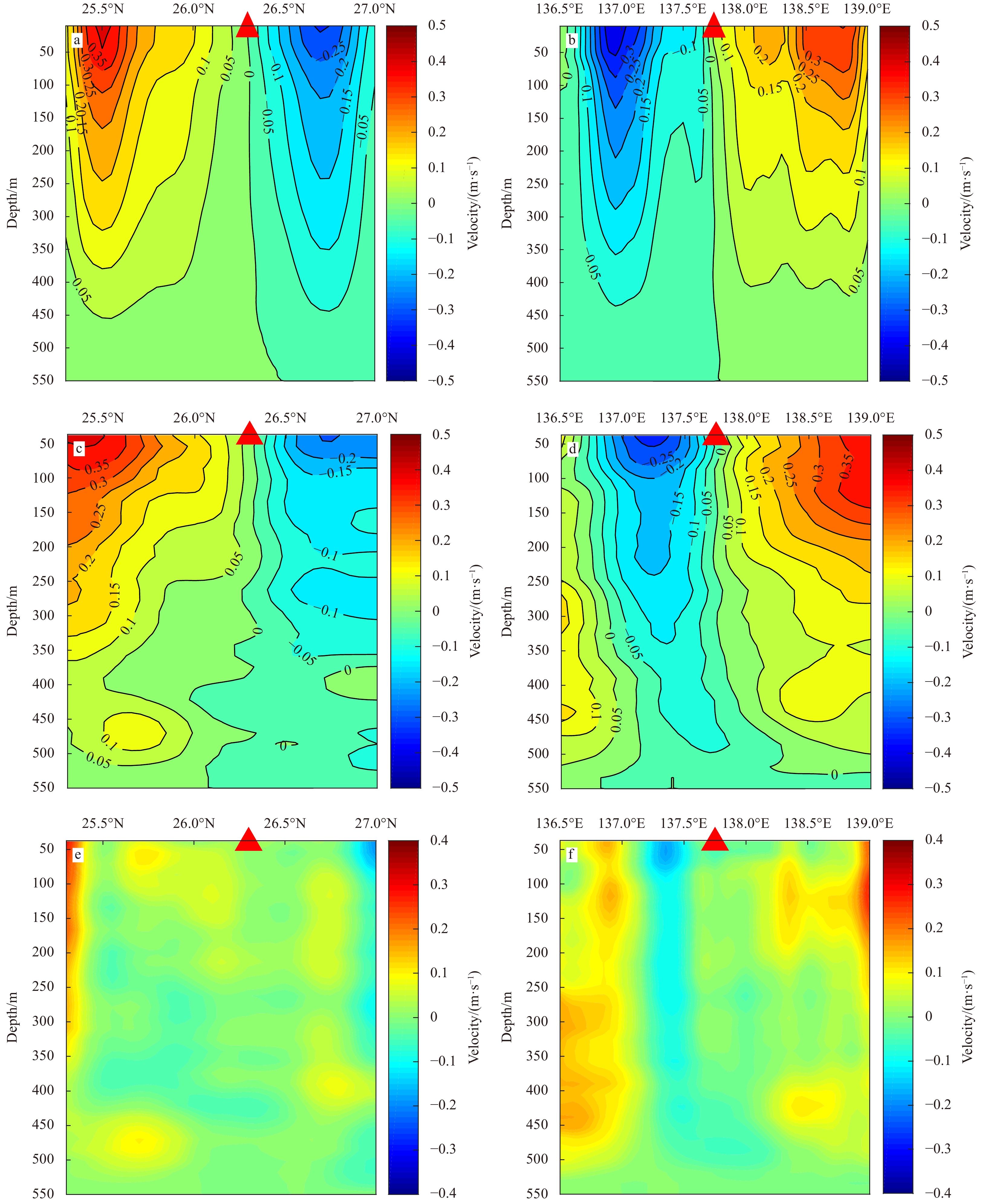
Figure  5.  The geostrophic anomaly velocity (a, b), revised ADCP velocity (c, d), ageostrophic velocity (e, f) on the meridional (a, c and e) and zonal sections (b, d and f) across the eddy center. The red triangle represents the position of the eddy center on the surface.

DownLoad: Full-Size Img PowerPoint

where α is the specific volume, P₀ is the reference level, and P represents the pressure. The reference depth is 550 m in this study, since 550 m is the maximum depth obtained by observation. The dynamic height anomaly H′ can be obtained by subtracting CARS2009 climatology of the same latitude and longitude on the same day from the in situ temperature and salinity data. The formula for calculating geostrophic current anomaly V′ (u′, v′) is as follows:

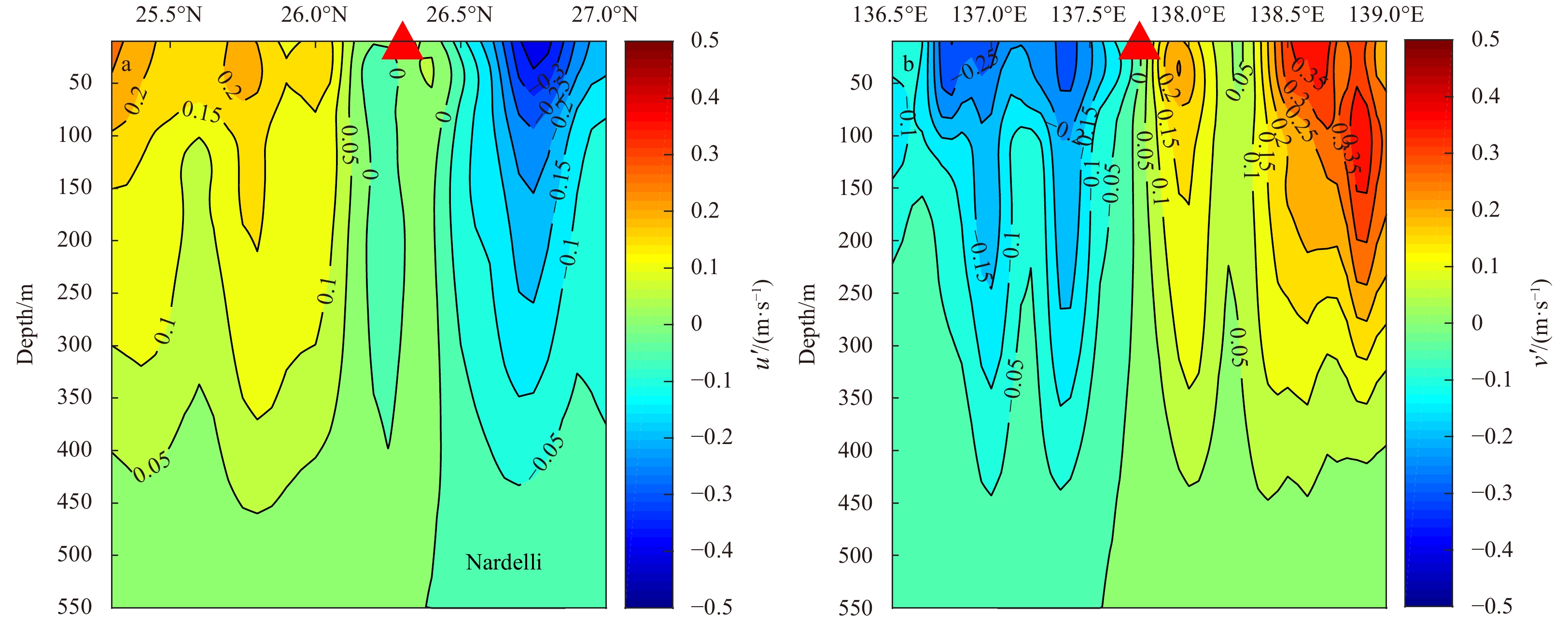
where u′ and v′ are the zonal and meridional components of V′, respectively; and f is the Coriolis parameter at the central latitude of the study area. The dynamic height anomaly H′ was computed from the temperature and salinity field. The geostrophic current anomaly has a counter clockwise rotation structure in the cyclonic eddy, so the zonal and meridional velocity anomalies u′ and v′ on both sides of the eddy center are opposite. V′ is largest on the surface, approximately 0.5 m/s, and it decreases with depth. It still maintains a speed of about 0.05 m/s at 400 m. The maximum geostrophic current on the south side of the eddy reaches 0.35 m/s, which is stronger than that on the north side. Additionally, the current on the west is slightly stronger than that on the east.

Figures 5c–f are the revised ADCP velocity and the ageostrophic velocity profiles on the zonal and meridional sections across the eddy center, respectively. Compared with geostrophic velocity, the ADCP-derived velocity includes not only baroclinic velocity, but also barotropic velocity and some noise (due to the swing of ship). The velocity of 550 m level is subtracted from the ADCP velocity at each level to remove the barotropic velocity or noise. The revised ADCP velocity in Figs 5c and d can be expressed as: V_{ADCP_new (z)}=V_{ADCP (z)}−V_{ADCP (550 m)}, z represents the depth. Then, the ageostrophic velocity in Figs 5e and f can be obtained by subtracting the geostrophic velocity from the revised ADCP velocity. From Figs 5c and d, it can be seen that the size and the distribution of revised ADCP velocity are similar to geostrophic velocity in Figs 5a and b. However, there is a small velocity extreme at a depth of 450–500 m in revised ADCP velocity (Fig. 5c). The ageostrophic velocity in Figs 5e and f is much less than the velocity in Figs 5a–d, and the velocity is only about 0.1 m/s. And the ageostrophic velocity does not change much with depth. The ageostrophic speed is closely related to the vertical motion. Some diagnostics based on the quasi-geostrophic omega equation found that some changes in mesoscale eddies (such as eddy Rossby waves, distortions and eddy-eddy interactions) can also lead to strong vertical currents, whose size can even be close to the vertical flow caused by submesoscale processes (Ni, 2019). Nardelli (2013) also pointed out that the disturbance to the geostrophic balance results in the vertical motion of the eddy. The vertical motion may be the result of two combined components: isopycnal shoaling/deepening and ageostrophic motion along sloping isopycnal surfaces.

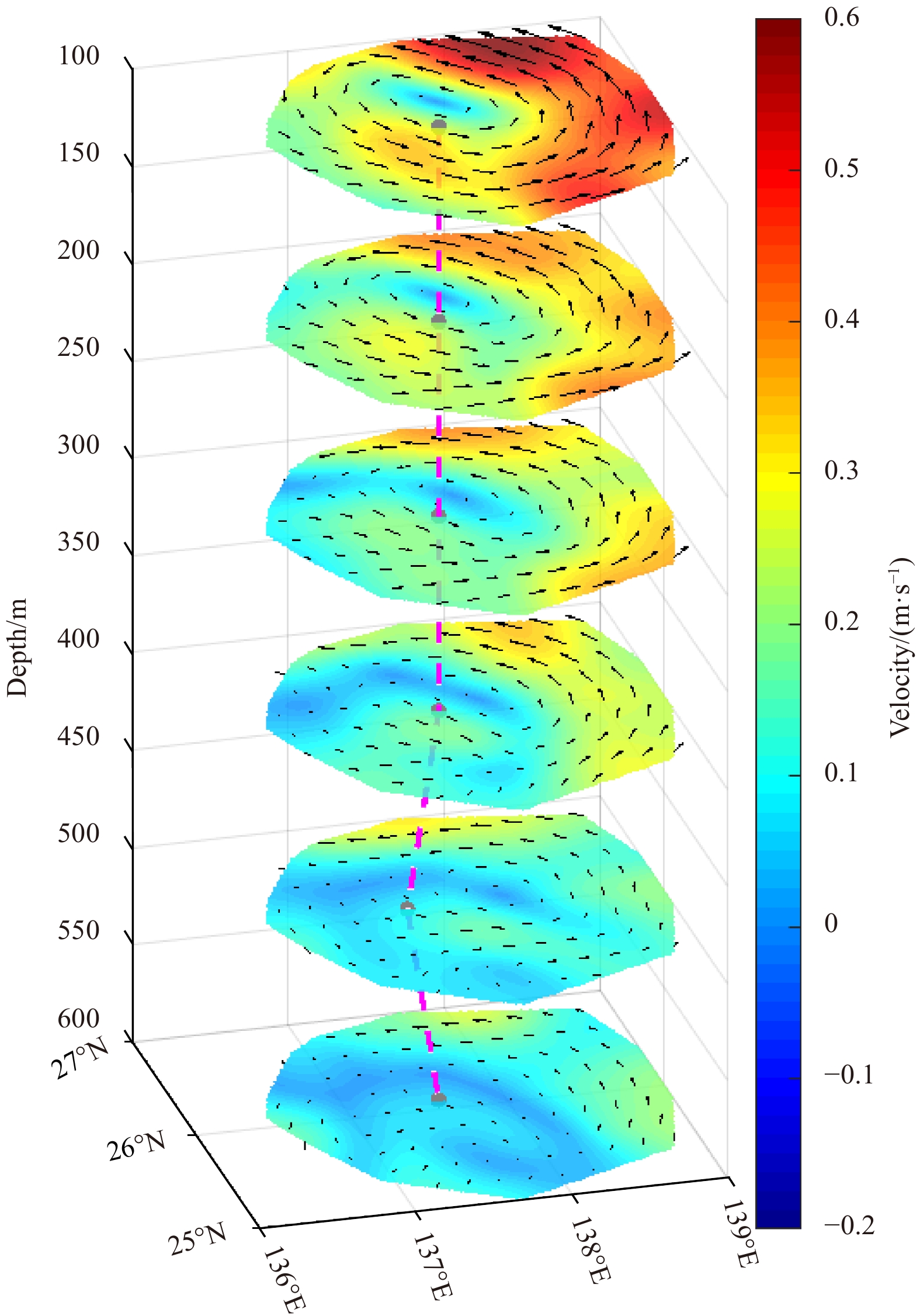
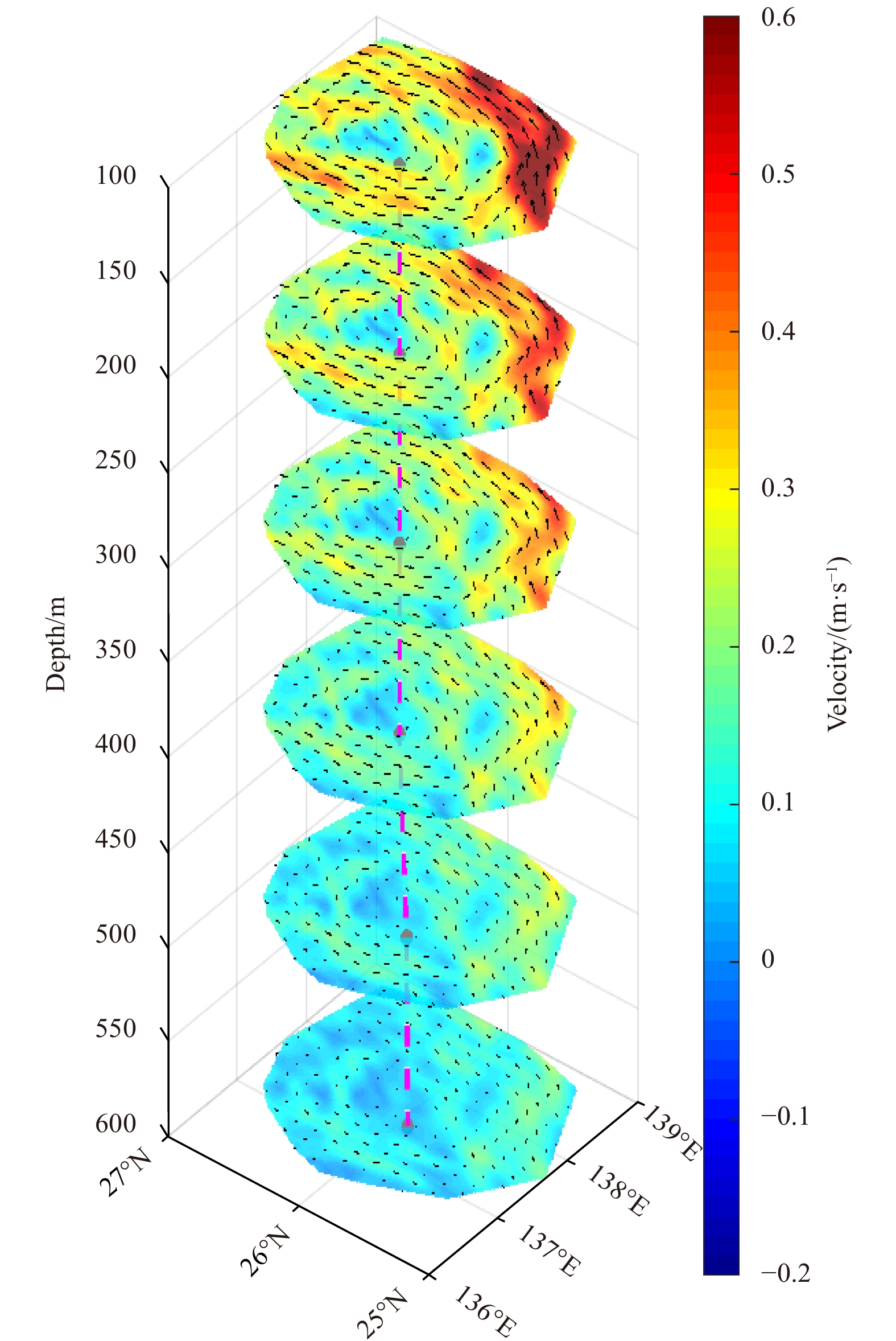
Figure 6 shows the cold eddy’s three-dimensional structure of the horizontal velocity. The flow field was obtained by interpolating the in situ measurement observed by ADCP into the grid with Divand method. The characteristics of the flow field mainly included the following. In the horizontal direction, velocity is weakest at the eddy center and increases with distance from the center. There is a distinct asymmetric cyclonic circulation structure within the range of the mesoscale eddy. The velocity is enhanced on the eastern side of the cold eddy due to the existence of a clockwise anticyclonic eddy on the east of the cold eddy. The enhancement of the velocity is caused by the interaction between the two eddies. In the vertical direction, the eddy is surface-intensified, and the velocity gradually decreases with the depth. The axis of the eddy is defined as the line connecting the minimum velocity in the central region of each layer. The axis of the cold eddy (pink line) here is basically vertically downward with a little tilt.

Figure  6.  The horizontal velocity with depths of 100 m, 200 m, 300 m, 400 m, 500 m and 600 m. The pink line represents the eddy axis.

DownLoad: Full-Size Img PowerPoint

3.3 The heat and salt transport caused by the eddy

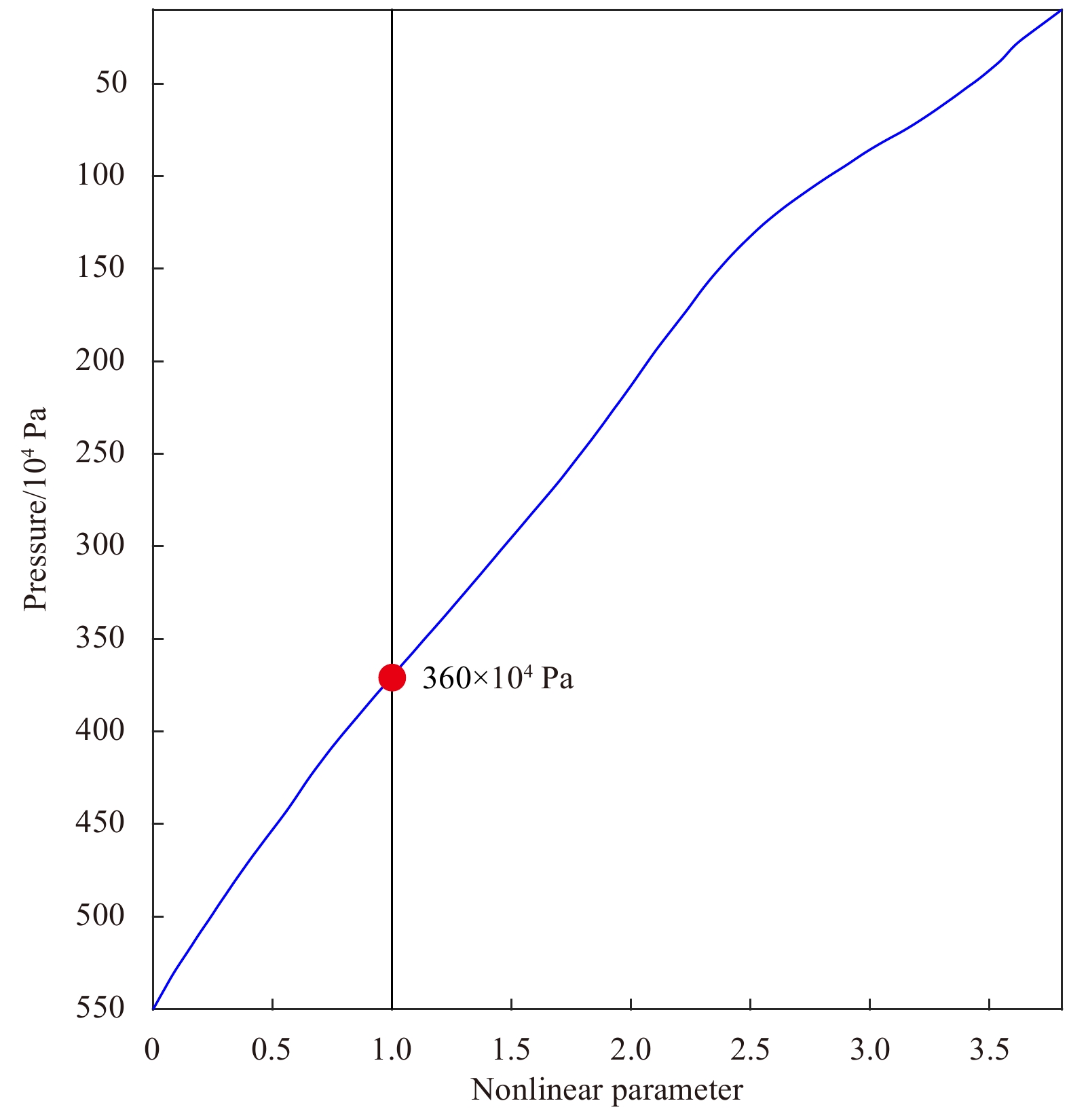
In order to estimate the heat and salt transport caused by the eddy, it is necessary to introduce two parameters: nonlinear parameter and trapping depth (Chaigneau et al., 2011). The nonlinear parameter is equal to the rotation speed divided by the moving speed of the eddy. When the nonlinear parameter is greater than 1, the water is considered to be nonlinear, and the eddy can carry the water in motion. The trapping depth means that the rotation speed of the eddy above this depth is greater than the average moving speed. Figure 7 shows the calculated nonlinear parameter changes with pressure, and the trapping depth is 360 m.

Figure  7.  Variation of nonlinear parameter with pressure.

DownLoad: Full-Size Img PowerPoint

The heat and salt transport caused by the eddy can be estimated by the available heat anomalies (AHA) and the available salt anomalies (ASA). The AHA and ASA of each layer are defined as:

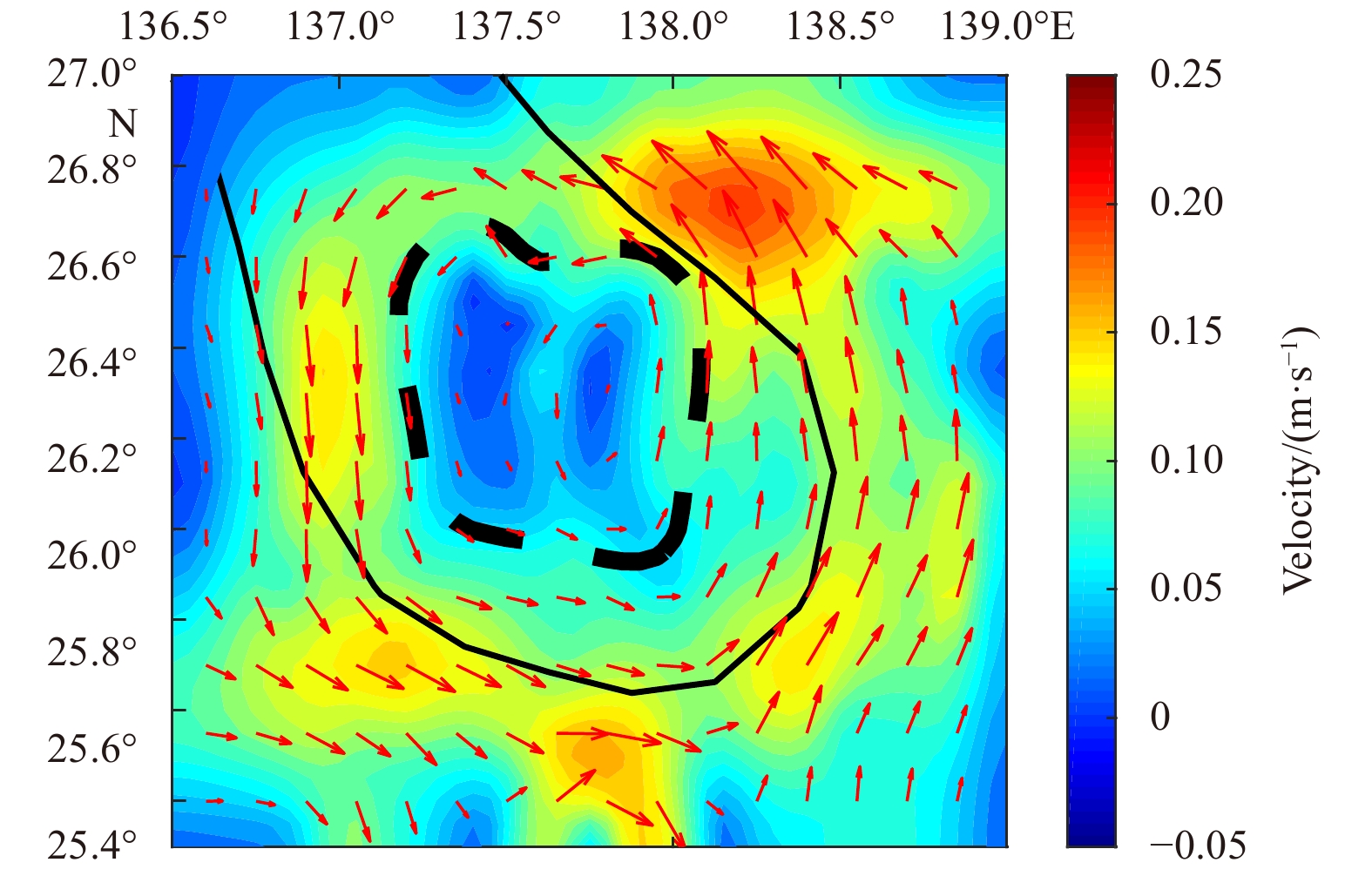
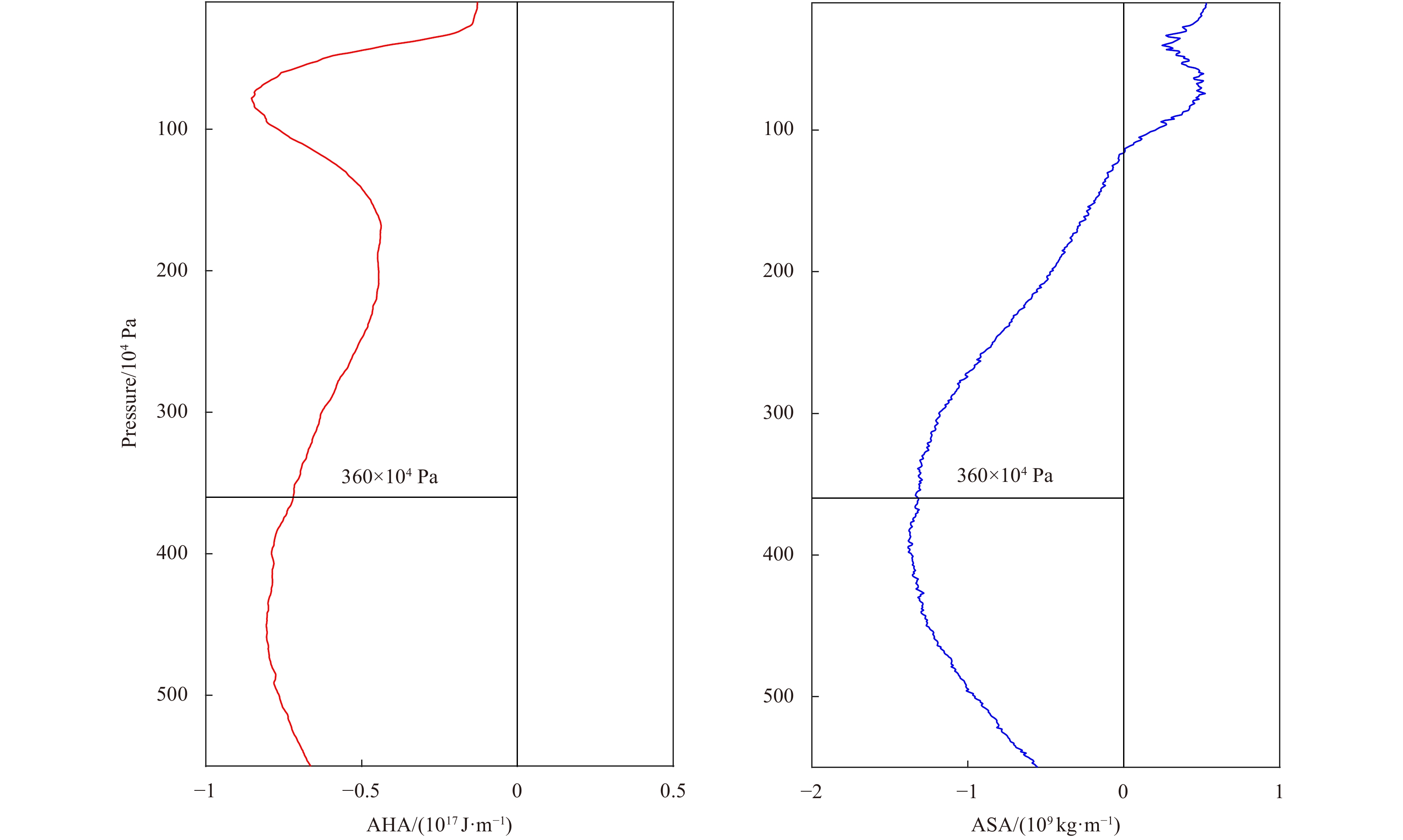
where ρ is the density (kg/m³), C_p is the specific heat capacity (4000 J/(kg∙K)), θ′ and S′ are the temperature and salinity anomaly fields, and A is the core area of the eddy, which is within the black dotted line in Fig. 8. The changes of AHA and ASA in each layer of the eddy with pressure are shown in Fig. 9. AHA has a minimum value above 100 m, and ASA has a minimum value near a depth of 360×10⁴ Pa. Integrated from the surface to the trapping depth, the total AHA and ASA can be obtained. The total AHA of this eddy is −1.95×10¹⁹ J, and the total ASA is −1.42×10¹¹ kg. Compared with the heat and salt transport calculated by Chaigneau et al. (2011) as − 5.5×10¹⁸ J and − 9.8×10¹⁰ kg, the heat and salt transport of the cyclonic eddy is slightly larger. The cyclonic eddy has a relatively strong transport capacity of heat/salt, this is because the trapping depth and nonlinear parameter of the cyclonic eddy are larger than those of Chaigneau et al. (2011).

Figure  8.  The horizontal section of the 300×10⁴ Pa layer V′ (m/s). The red arrow represents the velocity of the current, the black dashed line represents the boundary of the core area, and the black thin line represents the eddy edge.

DownLoad: Full-Size Img PowerPoint

Figure  9.  Variation of AHA and ASA with pressure. AHA: available heat anomalies, ASA: available salt anomalies.

DownLoad: Full-Size Img PowerPoint

4. Design and implementation of four-dimensional variational assimilation system

In this study, the ROMS (version 3.7, https://www.myroms.org) combined with the 4DVAR system were used to simulate the target mesoscale eddy.

4.1 Model configuration

In this study, the model domain covers part of the Northwest Pacific (18°–30°N, 124°–144°E), with a horizontal resolution of (1/20)°×(1/20)°, and 32 vertical σ levels. The bathymetry comes from GEBCO08 (0.5′×0.5′) with a minimum depth of 10 m and a maximum depth of 5 500 m. In the model, HYCOM reanalysis data were used as the initial state and boundary field (open boundary condition), while atmosphere forcing was derived from the ERA-5 reanalysis product. The model was integrated from September 25, 2019 to December 30, 2019 for realistic simulation, which started from the time of eddy generation and included the period for assimilation. The results of realistic simulation on November 13, 2019 (the first day of the survey) would be used as the initial field of assimilation. The data used for the realistic simulation are shown in Table 1. The model parameterization scheme includes the generic length scale (Warner et al., 2005), k–v vertical mixing scheme, and no slip boundary conditions.

Table  1.  Information of variables used for the realistic simulation, including their horizontal, temporal resolutions and sources

Variable	Horizontal resolution	Temporal resolution/h	Source
Heat flux	0.75°×0.75°	6	ERA-5
Freshwater flux	0.75°×0.75°	6	ERA-5
Wind stresses	0.25°×0.25°	6	ERA-5
T/S	(1/12)°×(1/12)°	3	HYCOM

 | Show Table

DownLoad: CSV

4.2 The 4DVAR experiment

In this study, the assimilation system is the primal formulation of incremental strong constraint 4DVAR (IS4DVAR) (Moore et al., 2011a). IS4DVAR is a non-sequential assimilation method, which finds the best model state that matches the observation in the assimilation window by minimizing the cost function (Thompson, 2010). The method also considers the errors of forcing fields and boundary conditions in the cost function and strives to obtain the global optimal simulation result (Powell et al., 2008). The corresponding cost function form is:

where x is the state vector $\left({T,\;S,\;\zeta,\;u,\;v} \right)$ during the assimilation window, x₀ is the initial condition, f is the atmosphere forcing (wind stress, heat flux), and b is the lateral open boundary condition. B_x, B_f, B_b, and R represent the error covariance matrices of the background field, surface forcing, lateral boundary conditions, and observations, respectively. The innovation vector d = y − H(x) represents the difference between observations and model analog in the observation space.

The starting time of assimilation is November 13, 2019, which is the first day of the survey. The total assimilation time is 3 d, and the timestep is 360 s. Observations including SSH, SST, and in situ measurement T/S data are used in the assimilation experiments. The detailed information of data assimilated into the experiment are as follows: (1) the daily SSH data from CMEMS with a horizontal spatial resolution of 0.25°×0.25°; (2) the daily SST data from CMEMS with a resolution of 0.25°×0.25°; (3) the in situ measurement of temperature and salinity data from eight sections. The observation errors from various sources are determined with the following standard deviations (Moore et al., 2011b): 2 cm for SSH, 0.48°C for SST, 0.18°C for in situ temperature T, and 0.01 for in situ salinity S.

The assimilation system process is presented in Fig. 10. The left dotted box represents the observations to be assimilated into the system, including the SSH, SST, and in situ T/S measurements. In the right dotted box, HYCOM data (used as the initial state and boundary field), and the ERA-5 dataset (used as atmosphere forcing) are imported into initial field module for realistic simulation. The result x^b is the initial condition of IS4DVAR. Observation data y^o and its error covariance R are connected to the assimilation system after assimilation pre-processing. Q, B_x, B_f, B_b are the error covariance of model, background, forcing and boundary, respectively. x^a is the result of 4DVAR assimilation system, which is the analysis field to analyze the three-dimensional structure of mesoscale eddies.

Figure  10.  The flow diagram of four-dimensional variational assimilation system.

DownLoad: Full-Size Img PowerPoint

4.3 Verification of assimilation experiment results

Before analysis, it is necessary to have a preliminary judgment on the effect of assimilation. To demonstrate how the assimilation improves the simulation result, the SLA, SST, temperature, and salinity field are compared with the observations.

4.3.1   Verification of SLA and SST

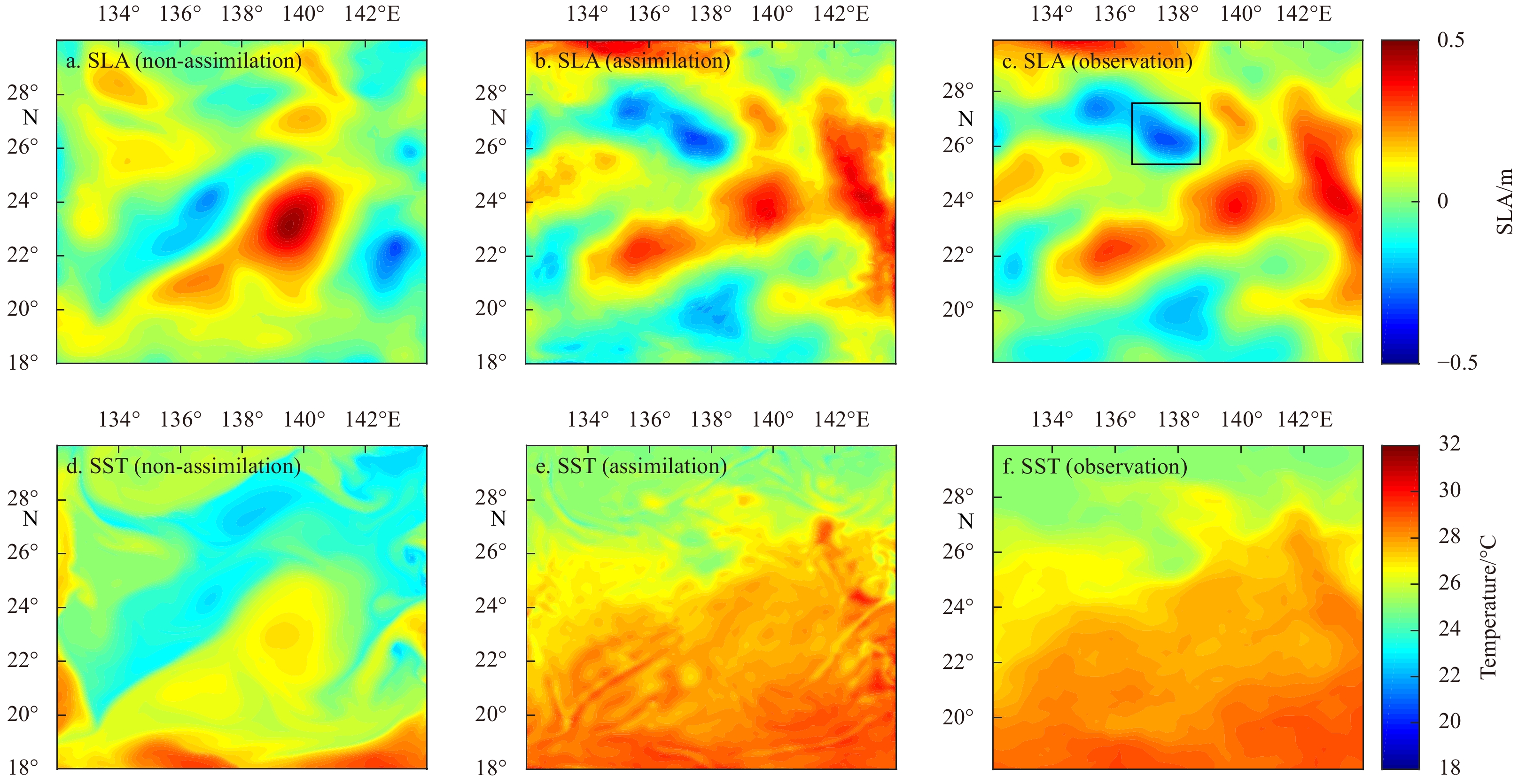
The comparison of the SLA is shown in Fig. 11. Figures 11a and b are two schemes of non-assimilation and assimilation, respectively, and Fig. 11c is the observation result from satellite altimeter. The negative area in the box in Fig. 11c is the target eddy of this study. The cold eddy is obviously reflected in assimilation scheme (Fig. 11b) and observation (Fig. 11c); however, the signal is very weak in non-assimilation scheme (Fig. 11a). For the non-assimilation result, it is quite different from observation. Only a few eddies can be found in Fig. 11a, and there is a negative area in the 142°–144°E region, which is opposite to the observation. Therefore, without assimilation, the model cannot accurately simulate the SSH in this experiment. The simulation effect of the SSH has been significantly improved after assimilation. The distribution of sea level anomalies in Fig. 11b is consistent with the observation, regardless of the eddy’s number or position. It is notable that the spatial resolution of the altimeter is (1/4)° and the model resolution of the two schemes is (1/20)°.

Figure  11.  Comparison of sea level anomaly (SLA), sea surface temperature (SST) between two schemes (non-assimilation, assimilation) and observations.

DownLoad: Full-Size Img PowerPoint

The comparison of SST has the similar conclusion. The non-assimilation scheme in Fig. 11d shows the signal of a strong warm eddy, but the overall temperature in the model area is low, especially in the southern region. The results of assimilation (Fig. 11e) are basically consistent with the observations (Fig. 11f), which also shows assimilation is very helpful to simulate the mesoscale eddy more accurately.

4.3.2   Verification of temperature and salinity field

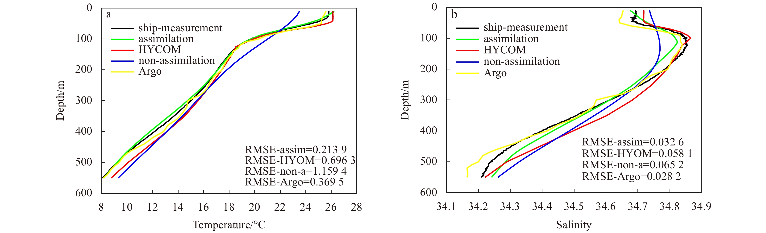
To verify the accuracy of the temperature and salinity of assimilation results, the research compare the non-assimilation results, assimilation results, in situ measurement by ship, HYCOM reanalysis data, and Argo profile. The No. 2903378 Argo float (ftp://ftp.argo.org.cn/pub/ARGO/global/core/) is just found at the location (26.137°N, 137.09°E) near the eddy center on the second day of assimilation, which satisfies requirements perfectly. In addition, the research respectively calculated the root mean square error (RMSE) to measure the deviation between each kind of data and the in situ measurement by ship. The calculation formula is as follows:

where z represents depth, x_{1, 2, ···, N} represents the observation, X_{1, 2, ···, N} represents the result which need to compare, and N is the total number of observations. The result is shown in Fig. 12.

Figure  12.  Comparison results of assimilation, HYCOM, non-assimilation, and Argo data with in situ measurement data. RMSE-assim, RMSE-HYCOM, RMSE-non-a, and RMSE-Argo represent the root mean square error (RMSE) between the in situ measurement by ship and the result of assimilation, HYCOM, non-assimilation and Argo, respectively. a. Temperature root mean square error of each kind of data between the in situ measurement by ship. b. Salinity RMSE of each kind of data between the in situ measurement by ship.

DownLoad: Full-Size Img PowerPoint

In Fig. 12a, the non-assimilation scheme has the largest deviation in the depth range; HYCOM is well simulated in the upper layer, but the overall temperature is higher below 300 m; both the assimilation scheme and Argo profile have a good temperature simulation in the experiment. It can be seen from the results of RMSE that the assimilation scheme is slightly better than Argo, followed by HYCOM, and finally the non-assimilation scheme. In Fig. 12b, the situation of the salinity profile is similar to the temperature. The simulation effect of the non-assimilation scheme still behaves poor. In the vicinity of the maximum salinity, the HYCOM simulation has the best effect; as the depth increases, all simulated salinity is larger than the observation; from the results of RMSE, the salinity of Argo profile is closer to the data by ship survey than other simulation results, and the assimilation scheme is also very close, followed by HYCOM and non-assimilation scheme. In general, the simulation effect of the non-assimilation scheme is improved significantly after assimilation, which is more accurate than HYCOM, especially under the depth of 300 m. The assimilation result is very close to the in situ measurement by ship and Argo profile. This result shows that the simulation of the mesoscale eddy’s three-dimensional structure in this study is relatively reliable.

5. Analysis of assimilation experiment results

5.1 Temperature and salinity field structure from assimilation results

In the assimilation results, the depth is extended from 550 m to 600 m. Figures 13a and c show the vertical temperature and salinity profile of the assimilation results, and Figs 13b and d show the vertical temperature and salinity anomaly, which are obtained by subtracting the CARS2009 climatology data from the assimilation results. The assimilation results have a good simulation effect on the eddy’s vertical temperature field, especially the dual-core structure is accurately described in Fig. 13b. The depths of the cores in the upper and deeper layers are basically consistent with the observation. The difference is that both cores showed greater temperature anomalies than observations, with the maximum value reaching approximately −4°C. In Fig. 13a, the isotherms exhibited upward bending as observations. The potential density line of 26 kg/m³ is shifted up approximately 50 m compared with the observation.

Figure  13.  Vertical temperature section (a), temperature anomaly (b), salinity section (c), and salinity anomaly (d) of the cold eddy from assimilation results in the zonal direction. The grey lines represent the potential density, and the numbers are the values of potential density. The black line represents an isoline with a value of 0.

DownLoad: Full-Size Img PowerPoint

The isohalines in Fig. 13c had similar characteristics to the observation. The core area of the negative salinity anomaly ranging from 200 m to 500 m in Fig. 13d is larger than that in observation of 250–500 m. Additionally, the salinity anomaly also exhibited a stronger eddy core structure. The negative anomaly in the core area reaches a salinity anomaly about −0.35.

The horizontal slice of temperature and salinity anomaly from assimilation at depths of 0 m, 100 m, 200 m, 300 m, 400 m and 500 m is shown in Fig. 14. The depth of 0 m here replaces 10 m of observation, because the model results cover the sea surface instead of the minimum depth of 10 m in observation. The anomaly value of temperature and salinity is also obtained by subtracting the CARS009 climatology data from assimilation result. The positive temperature anomaly in Fig. 14a at the surface is larger than observation in Fig. 4a. The isotherm is not close at 0 m and 100 m, but the clear dual-core vertical structure can also be reflected in this slice map. Negative value at 100 m is also obviously smaller than that of 0 m and 200 m. From the depth of 300 m, the absolute value of the negative temperature anomaly gradually increased, reaching the maximum value about −4°C between 400 m and 500 m. In Fig. 14b, the isohalines lines at 100 m are irregular and not close, but the distribution of salinity anomaly in vertical direction is in good agreement with observation. As the depth increases, the salinity anomaly gradually decreases, from the largest positive anomaly 0.1 at the sea surface to the largest negative anomaly −0.3 at 400 m. In general, the slice map from assimilation result can reflect the three-dimensional characteristics of the cold eddy.

Figure  14.  The slice map of temperature (a) and salinity (b) anomaly from assimilation result with depths of 0 m, 100 m, 200 m, 300 m, 400 m and 500 m.

DownLoad: Full-Size Img PowerPoint

5.2 The three-dimensional structure of velocity

The zonal and meridional components of geostrophic current anomalies u′ and v′ are shown in Fig. 15. The geostrophic current is calculated from the temperature and salinity field of the assimilation results. The highest velocity in Fig. 15 is 0.35 m/s. When compared with the observation results, the velocity of the northward and eastward currents is relatively higher. There are some differences between the assimilation and the observation results. In the observation results (Fig. 5), there is only one velocity maxima of zonal velocity anomaly u′ (Fig. 5a) and two unobvious velocity extremum near the eddy center of meridional velocity anomaly v′ (Fig. 5b), and their influence depth is very small, reaching only about 50 m. However, in the assimilation result (Fig. 15), there are two obvious velocity maxima in the horizontal direction from center to edge of the eddy. The reason for this phenomenon may be related to the temperature and salinity field from assimilation result, which used to calculate the geostrophic flow. It can be roughly seen from the temperature and salinity slice of assimilation result (Fig. 14) that there are two extreme values in the eddy center area of 200–500 m depth in the salinity anomaly slice, and two extreme values at the depth of 300 m in the temperature anomaly slice. This may be the reason why the geostrophic current in Fig. 15 has two velocity maxima.

Figure  15.  Zonal (a) and meridional (b) components of geostrophic current anomalies u′ and v′ from the assimilation result. The red triangle represents the location of the eddy center.

DownLoad: Full-Size Img PowerPoint

The cold eddy’s three-dimensional structure of the horizontal velocity from assimilation result is presented in Fig. 16. To show the effect of assimilation, ‘NAN’ was assigned to the grid points in the model data where the value is ‘NAN’ in the observation. The velocity field also remains the asymmetric in the horizontal direction, and the velocity is enhanced on the southeast side, which is different from the east side of the observation. The lowest velocity in each depth layer is also at the center. The characteristics of velocity in the vertical direction are consistent with the observation. The velocity decreases gradually with depth and the axis of the eddy is basically vertically downward. Compared to the assimilation results of temperature and salinity, the error of the velocity field from assimilation is larger, as the flow field observed by ADCP is not assimilated into the system.

Figure  16.  Horizontal velocity from the assimilation result with depths of 100 m, 200 m, 300 m, 400 m, 500 m and 600 m. The pink line represents the eddy axis.

DownLoad: Full-Size Img PowerPoint

5.3 Vertical motion in the mesoscale eddy

The vertical motion in the mesoscale eddies plays an important role in the ocean circulation and ocean-atmosphere interaction. Horizontal velocities in the ocean are typically orders of magnitude greater than vertical velocity, so it is difficult to measure the vertical velocity directly (Martin and Richards, 2001; Nardelli, 2013). In fact, due to the limitation of horizontal coverage and time sampling, the data obtained by traditional ship survey cannot reflect the vertical motion very well. In the assimilation experiment, the temperature/salt profiles were assimilated into the system, but the flow field by ADCP was not. T/S profiles play a limited role in adjusting the velocity field. Therefore, vertical velocity field needs the diagnostic analysis based on the high-resolution assimilation output result.

According to Hoskins et al. (1978), the Omega equation can be used to diagnose the vertical velocity in geostrophic velocity field. The Omega equation is as follows:

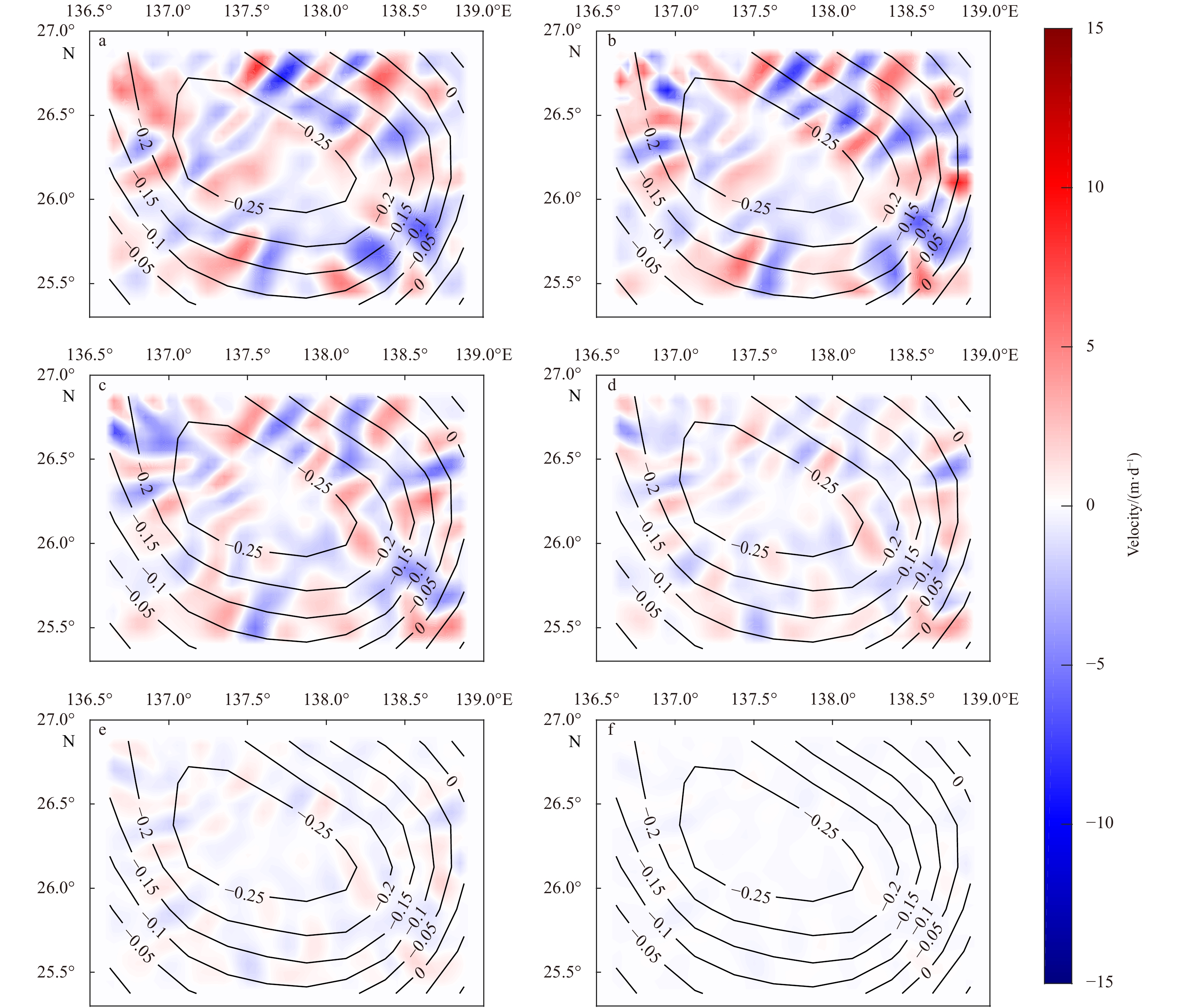
where f₀ and β represent Coriolis parameter and its variation with latitude respectively. w is the vertical velocity, and Q_x and Q_y in Eq. (16) are the X component and Y component of Q vector respectively. ${{{V}}_{\rm{g}}} = ({u_{\rm{g}}},{v_{\rm{g}}})$ represents the geostrophic velocity, N is the Brunt Vaisala frequency, and both are three-dimensional fields. It is assumed that the vertical velocity is zero at all boundaries. Through the Jacobian iteration method (Nardelli, 2013; Qiu et al., 2020), the vertical velocity was computed for the eddy region. To explore the vertical motion in the eddy, the vertical velocity from 100 m to 1 000 m is presented in Fig. 17. The positive (red) and negative (blue) value represent upward velocity and downward velocity, respectively.

Figure  17.  Vertical velocity fields at 100 m (a), 200 m (b), 400 m (c), 600 m (d), 800 m (e) and 1 000 m (f). The color shading represents the magnitude of the vertical velocity, and the black contours represent the sea level anomaly.

DownLoad: Full-Size Img PowerPoint

In general, the magnitude of the vertical velocity of the ocean is about O (10^–2) m/d. Due to the existence of mesoscale eddies, the intensity of vertical velocity field in Fig. 17 is significantly enhanced, and the maximum vertical velocity can reach nearly 10 m/d. The present results reveal a complex pattern of azimuthal oscillation, which regulates the evolution of the cyclone, and there are obvious signals in the core and periphery of the eddy (Nardelli, 2013). These signals are compatible with the propagation of potential vorticity (PV) anomalies along the radial gradient of PV, also called vortex Rossby wave (VRW) in the literature (McWilliams et al., 2003). VRW plays an important role in atmospheric research, for example, it is used to describe the development of the hurricane spiral band. However, it is difficult to observe vortex Rossby wave (VRW) in the ocean due to the sampling limitation of observations. It is mainly shown by theoretical demonstration and numerical models. In these theoretical demonstration and numerical models, VRW often shows the emergence of multipolar patterns of vertical velocity, with a maximum value on the periphery of the eddy (Nardelli, 2013). In the vertical direction, the vertical velocity gradually decreases with depth after 400 m and its distribution remains basically unchanged.

Figure 18 presents the vertical velocity field in zonal and meridional transects crossing the eddy center (26.28°N, 137.54°E). The upwelling (red) is dominant in the center area of eddy, which accords with characteristics of the cyclonic eddy. Additionally, the maximum vertical velocity is distributed on the edge of the eddy. At the edges of mesoscale eddies, submesoscale processes such as fronts, drawing, and small eddies are usually abundant. As the geostrophic balance is broken, these submesoscale processes can generate vertical currents of the order of 10 m/d (Ni, 2019). Zhang et al. (2020a) explored the submesoscale dynamics of the northwestern Pacific subtropical countercurrent region by deploying two nested mesoscale- and submesoscale-resolution mooring arrays. The results show the submesoscale features, including large vertical velocities (with magnitude of 10–50 m/d) and strong ageostrophic kinetic energy revealed in the upper 150 m. Moreover, some simulational results show that submesoscale features with strong vertical motion larger than 10 m/d (Sasaki et al., 2014) and submesoscale processes play an important role in vertical transport (Zhong et al., 2017; Zhang et al., 2020b). For example, Zhang et al. (2020b) used the output of the (1/30)° ocean model to study the spatiotemporal characteristics and generation mechanism of the submesoscales in the northeastern South China Sea. The simulation results show that the strong vertical velocity is about O (10–100 m/d). It is worth mentioning that the wind field can also generate significant vertical velocity by promoting submesoscale processes (Mahadevan et al., 2008; Mahadevan, 2016). The depth of influence of the vertical flow caused by the submesoscale process generally does not exceed a few hundred meters (McGillicuddy et al., 2007). In the vertical direction, maximum values appear between the surface and 400 m, and then the vertical velocity decreases gradually with depth. The vertical velocity patterns are vertically aligned within the eddy.

Figure  18.  Vertical velocity field in zonal (a) and meridional (b) transects crossing the eddy center.

DownLoad: Full-Size Img PowerPoint

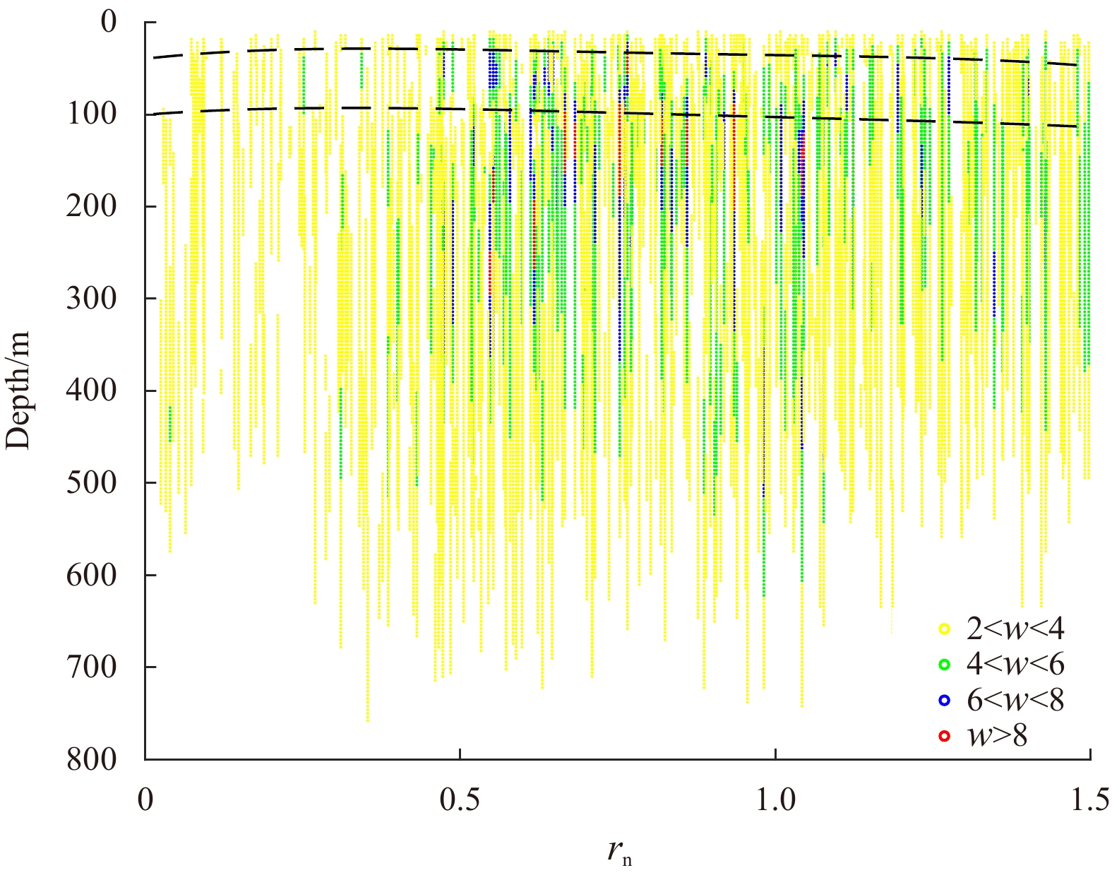
In addition, the distribution of vertical velocity from the eddy center to edge is investigated in Fig. 19, where r_n represents the normalized radius. The vertical velocity larger than 4 m/d is found to be distributed mainly in the range from 0.5 r_n to 1.0 r_n. The vertical velocity from the eddy center to 0.5 r_n is relatively small, basically no more than 6 m/d. The dotted lines represent the range of thermoclines calculated by the temperature gradient. In the vertical direction, the larger vertical velocity distribution ranges from the upper boundary of the thermocline to 500 m. The vertical velocity larger than 8 m/d is mostly distributed below the thermocline, while the vertical velocity above the thermocline is less than 4 m/d.

Figure  19.  Vertical distribution of vertical velocity from eddy center to edge, where r_n represents the normalized radius. The colors represent the different values of vertical velocity; the velocity field in the white regions in the figure is less than 2 m/d. The dotted lines represent the range of thermoclines.

DownLoad: Full-Size Img PowerPoint

5.4 Property of water mass carried by the eddy

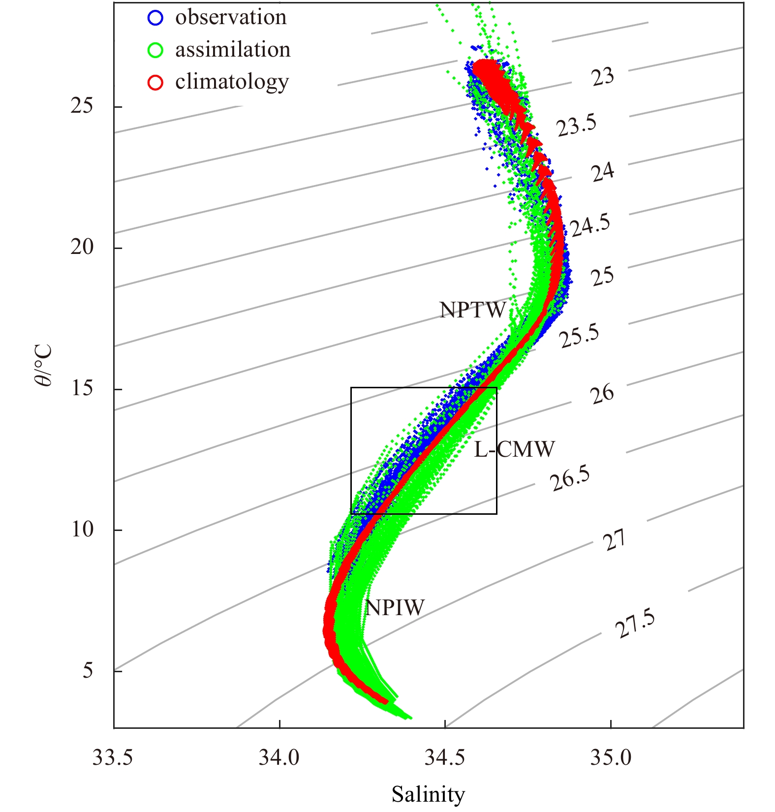
Due to the nonlinearity of the mesoscale eddy, it will carry the water mass when it translates during its life cycle (Zhang et al., 2014; Early et al., 2011). Therefore, the θ-S diagram can be used to study the nature of the water mass carried by the cold eddy. The θ-S diagram (Fig. 20) was derived from the observation (blue dots), assimilation (green dots), and CARS2009 climatology data (red dots). The maximum salinity represents subsurface high-salinity NPTW, the average salinity of NPTW is about 34.87 with a potential density about 22.5–25.5 kg/m³. The salinity minimum of the curve represents low-salt NPIW (θ=10–22°C, S=34.2–35, σ_θ=26.6–27.1 kg/m³). Between the subsurface layer and the middle layer is the STMW (θ=16.0–21.5°C, S=34.65–34.95, σ_θ=24.2–25.6 kg/m³) (Dong et al., 2017). The θ-S graph also showed a clear signal of light-central model water (L-CMW) (θ=10.0–16.0°C, S=34.44–34.65, σ_θ=25.4–26.3 kg/m³). Although L-CMW is mainly in the 33°–39°N region, the reason may be that the L-CMW’s formation area moves southeastward, crossing the Kuroshio Extension axis (Oka et al., 2011).

Figure  20.  Mean potential temperature-salinity characteristics of the water mass. The θ-S diagram is derived from observation (blue dots), assimilation (green dots), and CARS2009 climatology (red dots). The grey lines represent potential density. The range of water mass properties carried by the eddy is within the box. NPTW: North Pacific Tropical Water, NPIW: North Pacific Intermediate Water, L-CMW: light-central model water.

DownLoad: Full-Size Img PowerPoint

According to the temperature and salinity anomaly profiles, the deep range of water masses carried by the eddy is considered to range approximately between 250–500 m. Within this depth range, the average temperature and salinity anomaly values Δθ, ΔS were −3°C, −0.2, respectively. Compared to the mesoscale eddy previously studied in this area (Dong et al., 2017), it is larger than the average temperature anomaly of −2°C and salinity anomaly of −0.1. In this study, the transported water mass remained in the potential density layer of 25.5–26.5 kg/m³ throughout the life cycle, which indicates that the water mass trapped in the eddy core remains in a relatively stable state. Based on the previous features revealed by the three-dimensional structure, the temperature of the water mass in the core area is about 9–15°C and the salinity is about 34.2–34.6. Therefore, the range of water mass properties carried by eddy is within the box in Fig. 20.

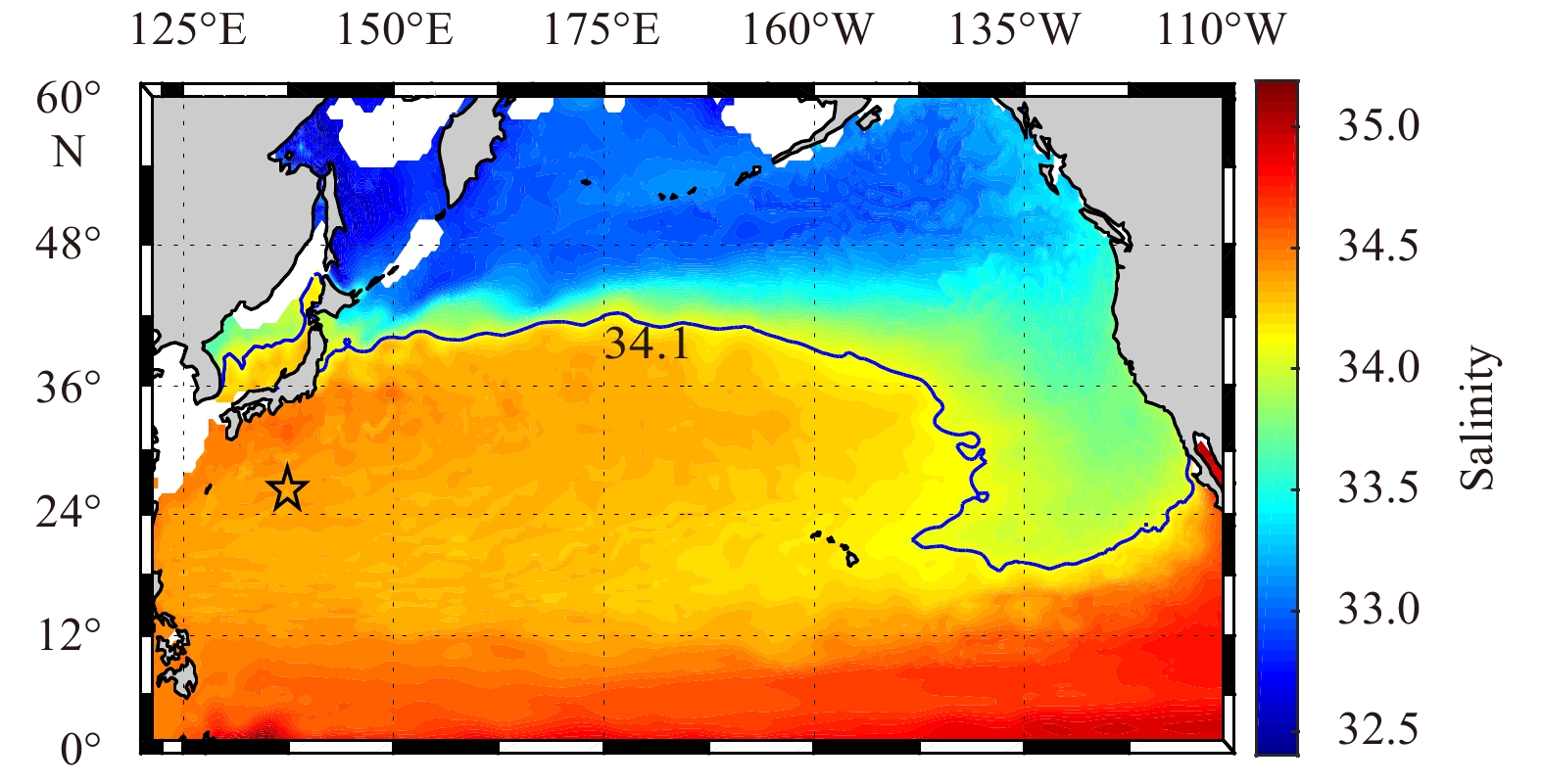
In order to find out the source of the water mass carried by the cold eddy, the research has made further analysis. Zhang et al. (2015) used salinity and oxygen as passive tracers under the permanent thermocline to track the Kiddies they observed. Li et al. (2017) also traced the origin of cold core Kiddies based on the distribution of S on the isopycnal layer. This study tries to trace the origin of the water mass carried by the eddy based on the average S distribution on the isopycnal layer. Firstly, it is assumed that the eddy moves along the isopycnal layer, and its water mass properties remain unchanged during the movement. Secondly, the minimum salinity observed in the cold eddy is the typical value of the eddy core (Zhang et al., 2015). It can be determined whether it is different from the surrounding water masses by observing the distribution of the minimum salinity. The core of the cold eddy observed in this study is distributed near the potential density layer of 26 kg/m³. Figure 21 shows the average distribution of salinity on the 26 kg/m³ isopycnal layer. The salinity data comes from the CARS2009 climate data. The minimum salinity of the eddy core is 34.1. In Fig. 21, the salinity contour (34.1) extends from 38°N on the east coast of Japan to around 30°N on the west coast of North America on this isopycnal layer. From the east coast of Japan to the range of 175°E, the contour has a northward trend, and east of 175°E begins to deflect to the south. The salinity contour shows a good correspondence with the Subarctic Front (SAF) in the North Pacific from the east coast of Japan to the range of 175°E. Therefore, it is speculated that the water mass inside the cold eddy originates from the SAF area of the North Pacific, or the northern boundary of the subtropical gyre.

Figure  21.  Distributions of salinity in the North Pacific on the 26σ₀ surface. The blue line denotes the contours of 34.1. The star indicates the position of the observed eddy.

DownLoad: Full-Size Img PowerPoint

6. Conclusions

In this study, based on the observation and assimilation results, the three-dimensional structure of the cold eddy captured during a cruise in the Northwest Pacific is investigated. The conclusions are as follows.

(1) The eddy was generated at 24.6°N, 139.6°E on September 25, 2019, and died out at 28.6°N, 131.6°E on February 28, 2020, for a total of 157 d. During its life cycle, it moved generally northwest about 1 520.5 km. The radius of the eddy was 78.8 km with an average propagation velocity about 0.11 m/s during its life cycle.

(2) The temperature field of the mesoscale eddy had a dual-core structure. One core was at 50–150 m, and the other was between 250 m and 550 m. The average temperature anomaly of the two cores was about −3.5°C. The salinity anomaly core was between 250 m and 500 m, about −0.3. The horizontal velocity structure was axis-asymmetric and the axis of the eddy is basically vertically downward. The maximum velocity on the surface was 0.5 m/s.

(3) Based on the high-resolution assimilation output results, the vertical velocity within the cold eddy was diagnosed. The maximum vertical velocity can reach about 10 m/d, far greater than the normal magnitude of O (10^–2) m/d in the ocean. The horizontal distribution of the vertical velocity shows the azimuthal wave-like patterns, and its maximum value appears on the edge of the eddy. The larger vertical velocity is mainly distributed in the range of 0.5 to 1 time the normalized radius of the eddy.

(4) The water masses carried by the eddy had the range of temperature and salinity values of 9–15°C, and 34.2–34.6, respectively. Additionally, the potential density remained at 25.5–26.5 kg/m³. Based on the property of water mass, the origin of the cold eddy was considered from the SAF area of the North Pacific, or the northern boundary of the subtropical gyre.

(5) Assimilating the observation into the ROMS model by 4DVAR method was proved to be effective in reconstructing the mesoscale eddy. The assimilation effect was verified by SLA, SST, in situ measurement by ship, Argo profile and HYCOM reanalysis data. Therefore, the assimilation results are reliable and accurately describe the three-dimensional structure of the cold eddy.

Acknowledgements

Thanks to Qinbiao Ni for his assistance in the calculation of vertical velocity and revision of the manuscript.