Huabin Mao, Xiujun Sun, Chunhua Qiu, Yusen Zhou, Hong Liang, Hongqiang Sang, Ying Zhou, Ying Chen. Validation of NCEP and OAFlux air-sea heat fluxes using observations from a Black Pearl wave glider[J]. Acta Oceanologica Sinica, 2021, 40(10): 167-175. doi: 10.1007/s13131-021-1816-0
Citation:
Huabin Mao, Xiujun Sun, Chunhua Qiu, Yusen Zhou, Hong Liang, Hongqiang Sang, Ying Zhou, Ying Chen. Validation of NCEP and OAFlux air-sea heat fluxes using observations from a Black Pearl wave glider[J]. Acta Oceanologica Sinica, 2021, 40(10): 167-175. doi: 10.1007/s13131-021-1816-0
Huabin Mao, Xiujun Sun, Chunhua Qiu, Yusen Zhou, Hong Liang, Hongqiang Sang, Ying Zhou, Ying Chen. Validation of NCEP and OAFlux air-sea heat fluxes using observations from a Black Pearl wave glider[J]. Acta Oceanologica Sinica, 2021, 40(10): 167-175. doi: 10.1007/s13131-021-1816-0
Citation:
Huabin Mao, Xiujun Sun, Chunhua Qiu, Yusen Zhou, Hong Liang, Hongqiang Sang, Ying Zhou, Ying Chen. Validation of NCEP and OAFlux air-sea heat fluxes using observations from a Black Pearl wave glider[J]. Acta Oceanologica Sinica, 2021, 40(10): 167-175. doi: 10.1007/s13131-021-1816-0
Ocean College, Zhejiang University, Zhoushan 316021, China
2.
Key Laboratory of Science and Technology on Operational Oceanography, South China Sea Institute of Oceanology, Chinese Academy of Sciences, Guangzhou 510301, China
3.
Key Laboratory of Physical Oceanography, Ministry of Education, Qingdao 266100, China
4.
Pilot National Laboratory for Marine Science and Technology (Qingdao), Qingdao 266237, China
5.
School of Marine Sciences, Sun Yat-sen University, Guangzhou 510275, China
6.
School of Mechanical Engineering, Tiangong University, Tianjin 300387, China
7.
Tianjin Key Laboratory of Advanced Mechatronic Equipment Technology, Tiangong University, Tianjin 300387, China
8.
Institute for Advanced Ocean Study, Ocean University of China, Qingdao 266100, China
Funds:
The National Key R&D Program of China under contract Nos 2017YFC0305904, 2017YFC0305902 and 2017YFC0305804; the National Natural Science Foundation of China under contract No. 44006020; the Guangdong Science and Technology Project under contract No. 2019A1515111044; the Shandong Provincial Key Research and Development Program (Major Scientific and Technological Innovation Project) under contract No. 2019JZZY020701; the Wenhai Program of Pilot National Laboratory for Marine Science and Technology (Qingdao) under contract No. 2017WHZZB0101; the CAS Key Technology Talent Program under contract No. 202012292205.
Latent and sensible heat fluxes based on observations from a Black Pearl wave glider were estimated along the main stream of the Kuroshio Current from the East China Sea to the east coast of Japan, from December 2018 to January 2019. It is found that the data obtained by the wave glider were comparable to the sea surface temperature data from the Operational Sea Surface Temperature and Sea Ice Analysis and the wind field data from WindSat. The Coupled Ocean Atmosphere Response Experiment 3.0 (COARE 3.0) algorithm was used to calculate the change in air-sea turbulent heat flux along the Kuroshio. The averaged latent heat flux (LHF) and sensible heat flux (SHF) were 235 W/m2 and 134 W/m2, respectively, and the values in the Kuroshio were significant larger than those in the East China Sea. The LHF and SHF obtained from Objectively Analyzed Air-Sea Fluxes for the Global Oceans (OAFlux) were closer to those measured by the wave glider than those obtained from National Centers for Environmental Prediction (NCEP) reanalysis products. The maximum deviation occurred in the East China Sea and the recirculation zone of the Kuroshio (deviation of SHF >200 W/m2; deviation of LHF >400 W/m2). This indicates that the NCEP and OAFlux products have large biases in areas with complex circulation. The wave glider has great potential to observe air-sea heat fluxes with a complex circulation structure.
Heat fluxes at the air-sea interface include shortwave radiation, longwave radiation, latent heat flux (LHF), and sensible heat flux (SHF). The SHF and LHF at the air-sea interface are turbulent heat fluxes that have a major effect on the thermodynamics of the upper ocean (Hogg et al., 2009). They modulate the sea surface temperature (SST) (Barnier, 1998) and are influenced by wind speed (Yusup and Liu, 2020). Many reanalysis products have been developed, such as the National Centers for Environmental Prediction (NCEP), Objectively Analyzed Air-Sea Fluxes for the Global Oceans (OAFlux), and European Centre for Medium-Range Weather Forecasting (ECMWF) products. However, their accuracy still needs to be validated using in situ observations.
These products depend on measurements of SST, wind speed, and air parameters. Satellite retrievals of wind speed and humidity differences between the sea surface and 10-m height can be used to calculate turbulent heat flux (Kubota et al., 2002; Sun et al., 2003; Yu and Weller, 2007; Liu and Curry, 2006). In situ observations, such as from the global surface drifter array (Pinardi et al., 2019), the Voluntary Observing Ship Scheme (Smith et al., 2019), and the tropical moored buoy array (Ueyama and Deser, 2008), are also used to calculate turbulent heat flux. Studies (Zeng and Wang, 2009; Wang et al., 2013) have been focus on the turbulent heat fluxes developed by satellite (SCSSLH) in the marginal sea near China. They made the comparison with in situ observations and other five heat flux products. These validations are important for atmospheric and oceanic modelling. However, traditional observation tools are expensive and difficult to deploy.
Wave gliders are relatively inexpensive, lightweight tools for sea surface studies and are now widely used in oceanography. They are autonomous surface vehicles propelled via the conversion of ocean wave energy into forward thrust (Hine et al., 2009; Manley and Willcox, 2010; Sun et al., 2019). They conduct near-surface oceanic and atmospheric surveys using a suite of sensors mounted on the float and the submerged glider (Daniel et al., 2011; Villareal and Wilson, 2014; Mitarai and McWilliams, 2016; Thomson and Girton, 2017). van Lancker and Baeye (2015) used a wave glider in a shallow sandbank area in the Belgian part of the North Sea and found that it was useful for studying sediment transport. Mitarai and McWilliams (2016) used a wave glider to observe air-sea processes during a typhoon (equivalent to a category 4 hurricane) near Okinawa, Japan. The wave glider provided an updated and more complete view of actual air-sea interactions in a typhoon. Ko et al. (2018) used wave gliders to observe the sea surface water temperature and wave height. Chavez et al. (2018) demonstrated that an integrated instrument package on wave gliders measuring temperature, salinity, oxygen, pCO2, pH, and wind speed and direction is capable of mapping variability, at temporal (min) and spatial (km) scales, in coastal upwelling processes and the resulting biogeochemical transformations. High-rate, continuous sea surface height measurement was also demonstrated using an unmanned, self-propelled, surfboard-sized wave glider surface vehicle equipped with a Global Navigation Satellite System (GNSS) receiver and antenna (Penna et al., 2018). Pagniello et al. (2019) conducted coastal surveys of fish choruses and mapped their spatial distributions using an autonomous Liquid Robotics wave glider. Zhang et al. (2019) used a wave glider to autonomously track an oceanic thermal front. Multiple wind products have been compared to the first high-resolution in situ measurements of wind speed obtained from wave gliders deployed in the Southern Ocean (Schmidt et al., 2017).
In this study, data from the “Black Pearl” wave glider were used to obtain turbulent heat fluxes in the Kuroshio area. Section 2 describes the measurements and methods used to estimate LHF and SHF. Section 3 compares different heat flux products with wave glider observations. Section 4 discusses the possible causes of the discrepancies between different results and Section 5 summarizes the main findings of the paper.
2.
Data and method
2.1
Observation
The Black Pearl wave glider is a mobile ocean observation platform developed by the Ocean University of China and Tiangong University (Sun et al., 2019). The structural parameters of Black Pearl wave gliders are shown in Table 1. The sensors equipped on the wave glider include a pumped Glider Payload conductivity-temperature-depth (CTD) sensor from Sea-Bird Electronics and an Airmar 200-WX weather station (Table 2). The CTD sensors were located at 0.3 m depth and measured water temperature, salinity, and pressure every 10 min. A weather station was mounted at 1.2 m height and provided measurements of wind speed, wind direction, air pressure, and air temperature every 10 min.
Table
1.
Measured parameters of the Black Pearl wave glider
Observations were conducted for 38 days from December 22, 2018 to January 30, 2019. The wave glider was launched from the mouth of the Changjiang River and then moved freely with the Kuroshio (Fig. 1). SST data were derived from the Operational Sea Surface Temperature and Sea Ice Analysis (OSTIA), which uses satellite data provided by the Group for High Resolution Sea Surface Temperature (GHRSST) project, together with in situ observations, to determine the SST. The product is produced using a variant of optimal interpolation described by Martin et al. (2007). The study used the daily and (1/20)° (approx. 5 km) product.
Figure
1.
The Black Pearl wave glider (a) and wave glider path (b). The background data are OSTIA SST from January 30, 2019. The arrows indicate the locations of the wave glider for the corresponding date.
In this paper, the Coupled Ocean Atmosphere Response Experiment (COARE) 3.0 was used to calculate the SHF and LHF of the wave glider (downloaded from https://www.coaps.fsu.edu/COARE/flux_algor/). This method has been widely adopted in mid-latitudes. The COARE 3.0 algorithm is shown as follows:
where w is the vertial wind; x can be U and V wind components, the potential temperature θ, the water vapor specific hmidity q, or some atmospheric trace species mixing ratio; w′ and x′ represent the turbulent fluctuations; cx is the variable block transport coefficient; cd is the wind drag coefficient; Cx is the total transport coefficient; ∆X is the difference in the mean value of x at the air-sea interface; Xs is the mean value of x relative to ocean surface and S is the mean wind speed (relative to ocean surface), which is composed of a mean vetor part (U and V components) and a gustiness part (Ug):
where the subscript n is the neutral stability (ξ=0); Z is the measurement height of $ x(z)$; κ is the von Kármán constant; Z0x is the roughness length of x; andξ is the stability parameter from Eq. (6):
where T is temperature; g is the acceleration of gravity; $ {u}^{*}=\sqrt{-\overline {w{'}u{'}}} $ is the friction speed; $ {\theta }^{*}=-\overline {w{'}\theta {'}}/{u}^{*} $ is the friction temperature; and $ {q}^{*}=-\overline {w{'}q{'}}/{u}^{*} $ is the friction humidity.
$ {\psi }_{x} $ is the stability correction function from Eq. (7) (Fairall et al., 1996):
Other ancillary datasets including WindSet, NCEP, and OAFlux are used in the paper.
The WindSat Polarimetric Radiometer was developed by the Naval Research Laboratory Remote Sensing Division and Naval Center for Space Technology of the US Navy, and the National Polar-orbiting Operational Environmental Satellite System Integrated Program Office. It was launched on January 6, 2003 aboard the Department of Defense Coriolis satellite. WindSat was designed to demonstrate the capability of a fully polarimetric radiometer to measure the ocean surface wind vector from space. All of the ocean measurements are gridded onto a 0.25° map, and the 3-day averaged wind speed data were used.
Net shortwave radiation, net longwave radiation, LHF, SHF, humidity, and precipitation data were obtained from NCEP reanalysis products. The 6-h and 1.875°×1.875° resolution surface flux products were used.
The OAFlux (http://oaflux.whoi.edu/) SHF and LHF were used for validation. OAFlux provides a near real-time 1° global analysis from January 1958 onward.
3.
Results
3.1
Validation of wave glider-measured SST and wind speed
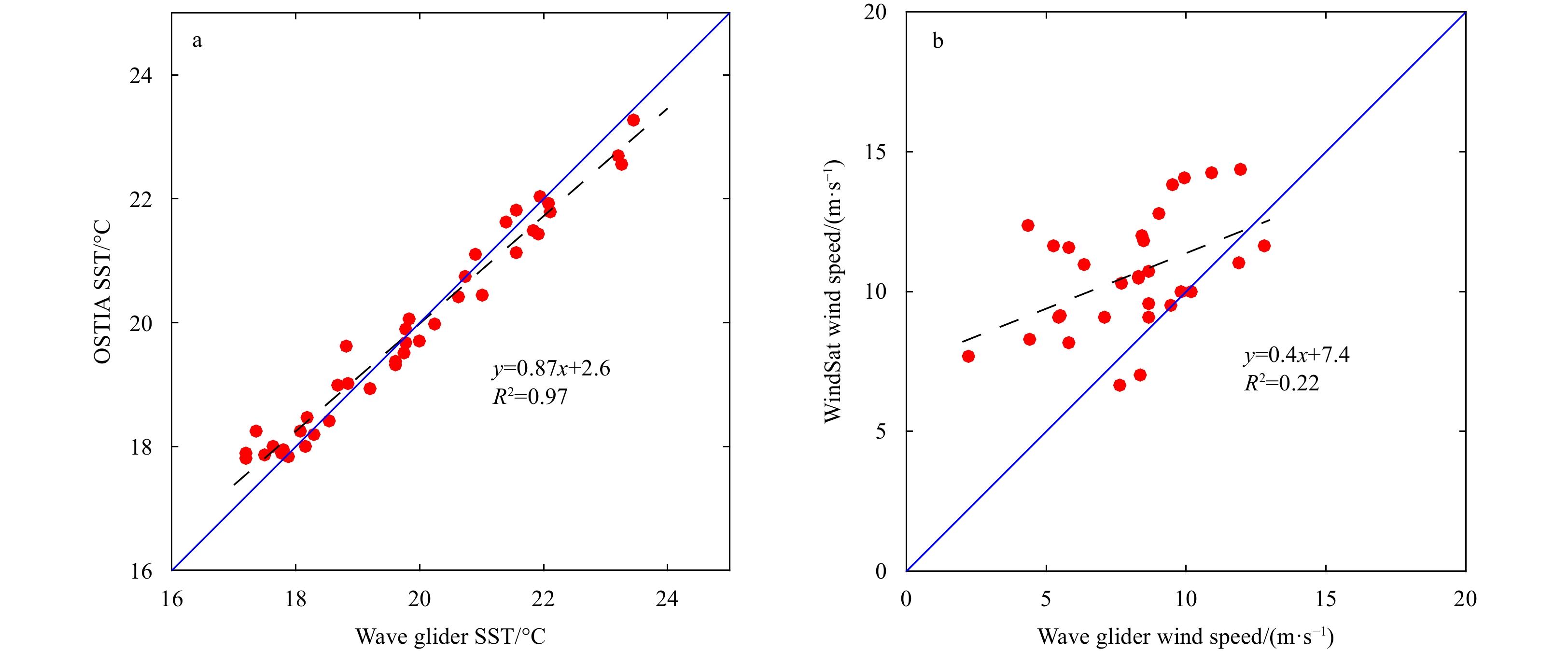
Figure 2a shows the comparison between the SST measured by the wave glider and that obtained by OSTIA. The linear correlation coefficient is more than 0.90, and the linear function is $ {y}_{0}=0.87{x}_{0}+2.6 $. In the temperature range of 18–22°C, the difference between wave glider-observed SST and OSTIA SST was small. When the SST was lower than 18°C, the satellite SST was higher than that measured by the wave glider; above 22°C, the satellite SST was lower than that measured by the wave glider. This may be due to differences in the depth of the measurements, or to the influence of mesoscale dynamic ocean processes.
Figure
2.
Scatter plots of wave glider SST and OSTIA SST (a) and wave glider wind speed and WindSat wind speed (b). The blue line is ${{{{y}}}}={{{{x}}}}$. The black dash line is the fitted line.
Figure 2b shows a comparison between the actual wind speed measured by the wave glider and the wind speed retrieved by WindSat. The wind field deviation caused by the speed of the wave glider was deducted, and the treatment method was consistent with that of the automatic weather station carried on the glider. In most cases, the WindSat wind speed was higher than that measured by the wave glider. This may have been due to the high temporal frequency of the real wind field.
3.2
Wave glider observed air-sea turbulent fluxes
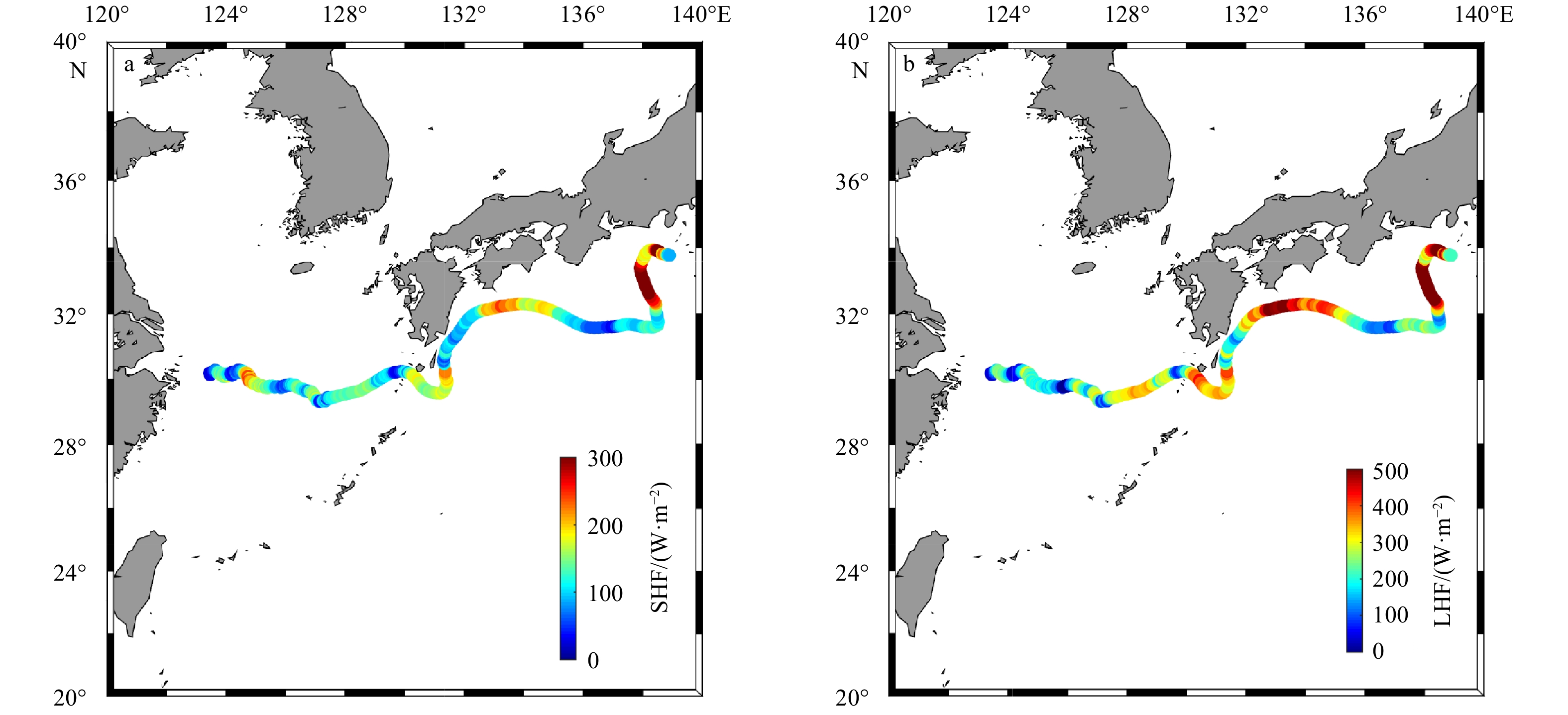
The wave glider moves from the Changjiang River Estuary to the Kuroshio, with a time span of more than one month and a space span of nearly 20°. Therefore, the wave glider observed fluxes have obvious spatial and temporal variability. Both SHF and LHF are greater than zero, indicating that the ocean releases heat to the atmosphere in observation time and space. The SHF mainly varies from 0 W/m2 to 300 W/m2, with an average value of 134 W/m2, while the LHF was larger, varying from 0 W/m2 to 500 W/m2, with an average value of 235 W/m2 (Fig. 3).
Figure
3.
Spatial distribution of SHF (a) and LHF (b) observed by the Black Pearl wave glider.
In the spatial distribution, the SHF had no obvious spatial distribution characteristics, and has large values on 124.5°E, 132°E, 133°E, and 137°E. The values of SHF were controlled by the difference between the air temperature and SST (Section 4). The LHF has similar spatial distribution characteristics as SHF. The spatial variation trend of SHF and LHF was consistent. In general, the SHF and LHF over the Kuroshio extension were larger than those over the East China Sea. For example, the observation results were divided into two parts at 130°E and average them separately. The average SHF was 118 W/m2 in the East China Sea and 160 W/m2 in the Kuroshio region. While the average LHF was 180 W/m2 in the East China Sea and 324 W/m2 in the Kuroshio region. These differences indicate that the stronger Kuroshio forces the atmosphere in the northern hemisphere in winter.
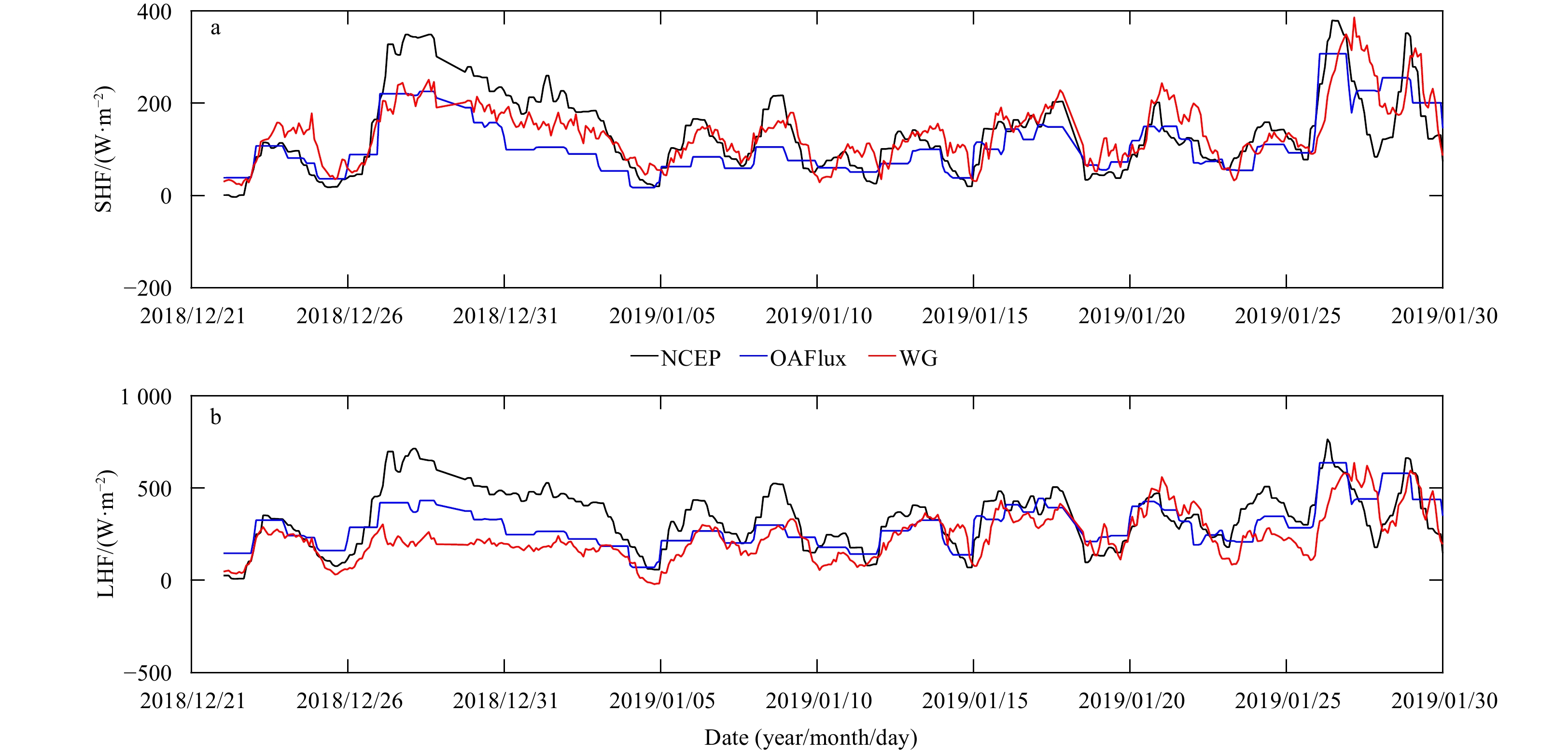
In the temporal distribution, SHF and LHF oscillate with time, and their changing trend was consistent (Fig. 4). The maximum value occurs after January 25, 2019 after the wave glider enters the Kuroshio area, which is shown in the Fig. 3. Also, the variations of SHF and LHF were controlled by the scatter difference in the air-sea interface.
Figure
4.
Time series of SHF (a) and LHF (b). The NCEP, OAFlux, and wave glider values are represented by black, blue, and red lines, respectively.
The temporal variations in heat flux data from NECP and OAFlux were equal to those of the wave glider calculation data (Fig. 4). However, there were some differences in magnitude, especially from December 28, 2018 to January 2, 2019, and from January 25, 2019 to January 31, 2019. NCEP showed a large deviation (the maximum sensible heat was about 150 W/m2, and the maximum latent heat was about 500 W/m2), while OAFlux showed a difference in sensible heat of 50 W/m2 and latent heat of 250 W/m2.
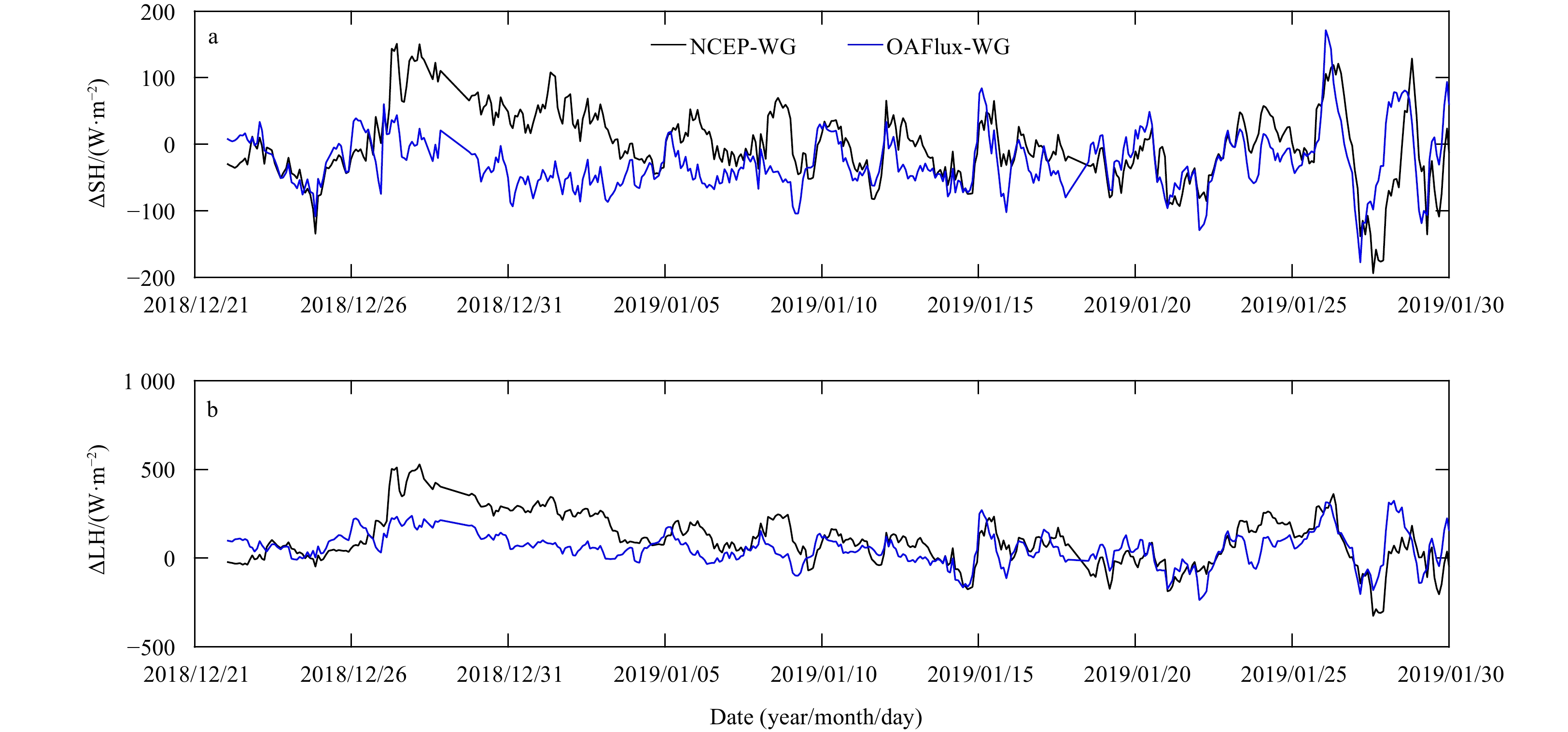
From December 28, 2018 to January 2, 2019, the SHF of OAFlux was close to that of the wave glider, whereas the LHF of OAFlux was slightly higher than that of the wave glider (Fig. 5). NCEP SHF and LHF were much higher than those of the wave glider. The differences in SHF and LHF between NCEP and the wave glider are represented as ΔSHNCEP-WG and ΔLHNCEP-WG, respectively; those between OAFlux and the wave glider are ΔSHOAFlux-WG and ΔLHOAFlux-WG. The average values of ΔSHNCEP-WG and ΔLHNCEP-WG were −1.8 W/m2 and 100.7 W/m2, respectively, while those of ΔSHOAFlux-WG and ΔLHOAFlux-WG were −26.3 W/m2 and 56.0 W/m2. The mean square deviations of SHF and LHF of NCEP were 57.0 W/m2 and 177.3 W/m2, respectively, while those of OAFlux were 53.3 W/m2 and 111.4 W/m2.
Figure
5.
Time series of differences in SHF (a) and LHF (b). The difference between the NCEP data and wave glider measurements is denoted by the black line, and that of OAFlux by the blue line.
Spatially, the largest deviation was in the East China Sea and the Kuroshio recirculation area. From January 26, 2019 to January 30, 2019 (Fig. 6), the amplitudes of ΔSHOAFlux-WG and ΔLHOAFlux-WG were high, resulting in alternating positive and negative discrepancies between OAFlux and the measured values. The wave glider operated in the Kuroshio recirculation zone during this period, where the Kuroshio main axis shifted frequently (Waseda et al., 2005). In addition, the Kuroshio Extension develops instabilities and sheds mesoscale eddies (Chelton et al., 2011). These active eddies play an important role in the transportation of ocean heat toward the poles (Dufour et al., 2015) and also affect the atmosphere (Frenger et al., 2013). Multiscale processes in this region influence the accuracy of turbulent heat flux reanalysis products because coarse reanalysis data cannot explain structures at or below the sub-mesoscale.
Figure
6.
Spatial distribution of differences in sensible heat flux (∆SH) between the NCEP and wave glider data (a), ∆SH between OAFlux and the wave glider (b), latent heat flux (∆LH) between NCEP and the wave glider (c), and ∆LH between OAFlux and the wave glider (d).
3.4
Factors leading to differences with NCEP and OAFlux datasets
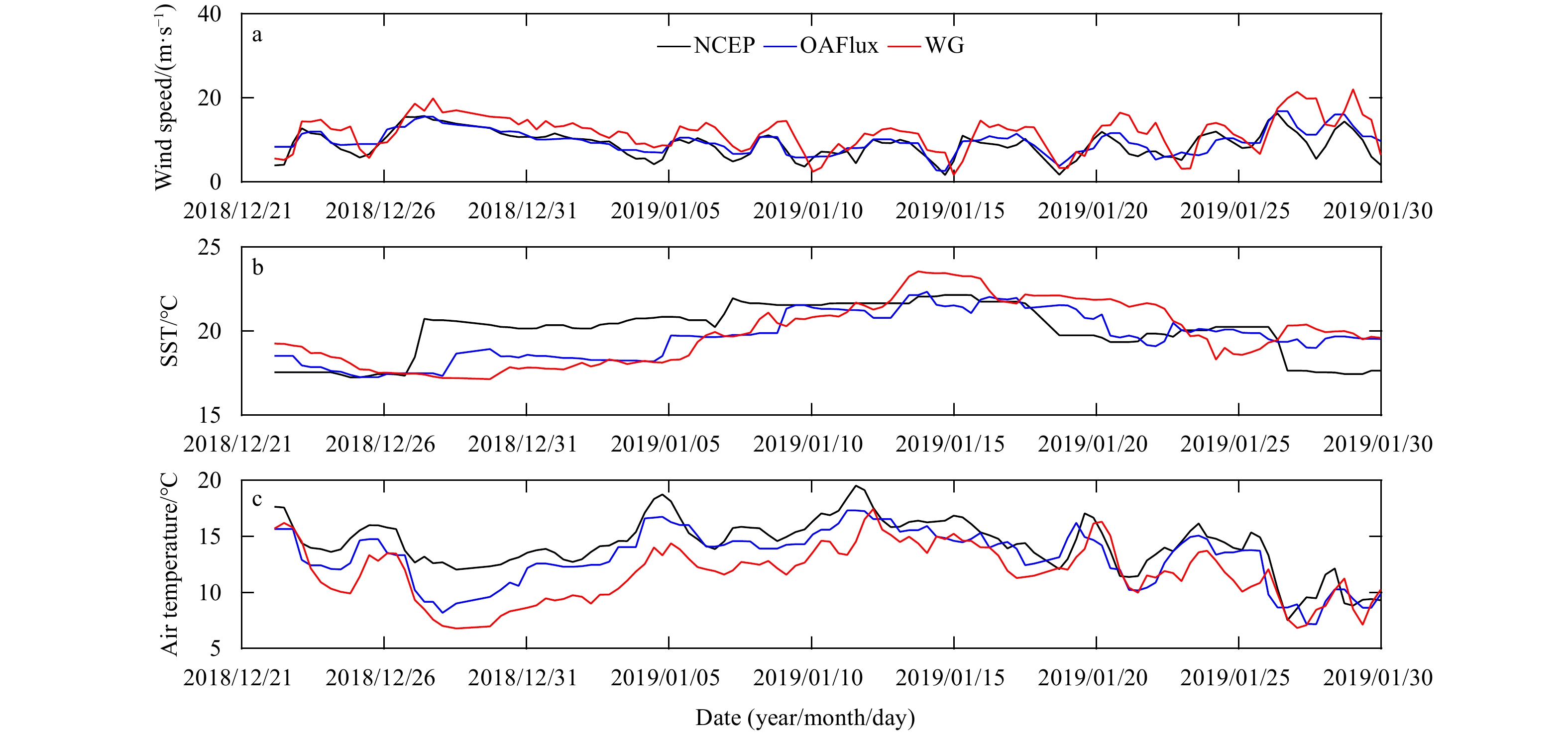
To examine the contributions of each variable in Eq. (1), the study compared the input wind speed, SST, air temperature data from NCEP, OAFlux, and the wave glider (Fig. 7).
Figure
7.
Display of time series of wind speed at 10 m (a), SST (b), and air temperature (c) during the measurements. The parameters derived from the NCEP, OAFlux, and wave glider data are black, blue, and red, respectively.
For the comparison with reanalysis wind speed data, the wave glider wind speed to 10-m height were converted. The variations in wind speed from NCEP and OAFlux were similar to those of the wave glider and consistent with those of SHF. The average wind speed difference between OAFlux and the wave glider was 1.94 m/s and the mean square deviation was 4.12 m/s, while those between NCEP and the wave glider were 2.65 m/s and 4.68 m/s, respectively. The greater/smaller mean bias of wind speed also corresponded to the greater/smaller biases of heat fluxes from NCEP/OAFlux.
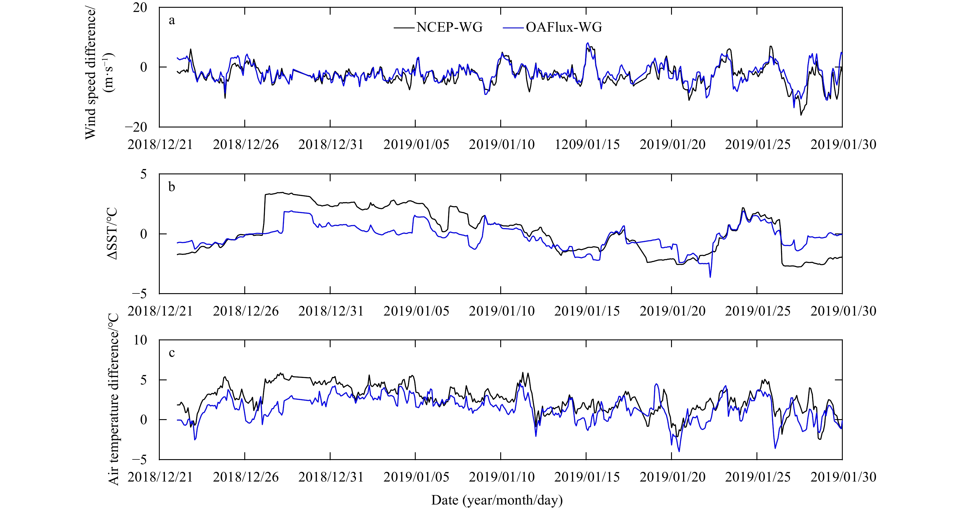
Both NCEP and OAFlux had higher SST and air temperature values than those observed by the wave glider from December 28, 2018 to January 2, 2019 (Figs 7b and c). From January 26 to 30, 2019, the SST and air temperature trends became complex. The fluctuation amplitude of ΔSSTOAFlux-WG at 0 was far lower than that of ΔSSTNCEP-WG, while the mean square deviations of ΔSSTOAFlux-WG and ΔSSTNCEP-WG were 0.99°C and 1.82°C, respectively (Fig. 8). The average air temperature difference of ΔATOAFlux-WG was 1.40°C, and the mean square deviation was 2.14°C, while those of ΔATNCEP-WG were 2.52°C and 3.07°C, respectively, which also contributed to the accuracy of OAFlux and NCEP.
Figure
8.
Display of time series of differences in wind speed at 10 m (a), SST (b), and air temperature (c) during the measurements. The difference between the NCEP and wave glider data is shown as a black line, and that between OAFlux and wave glider as a blue line.
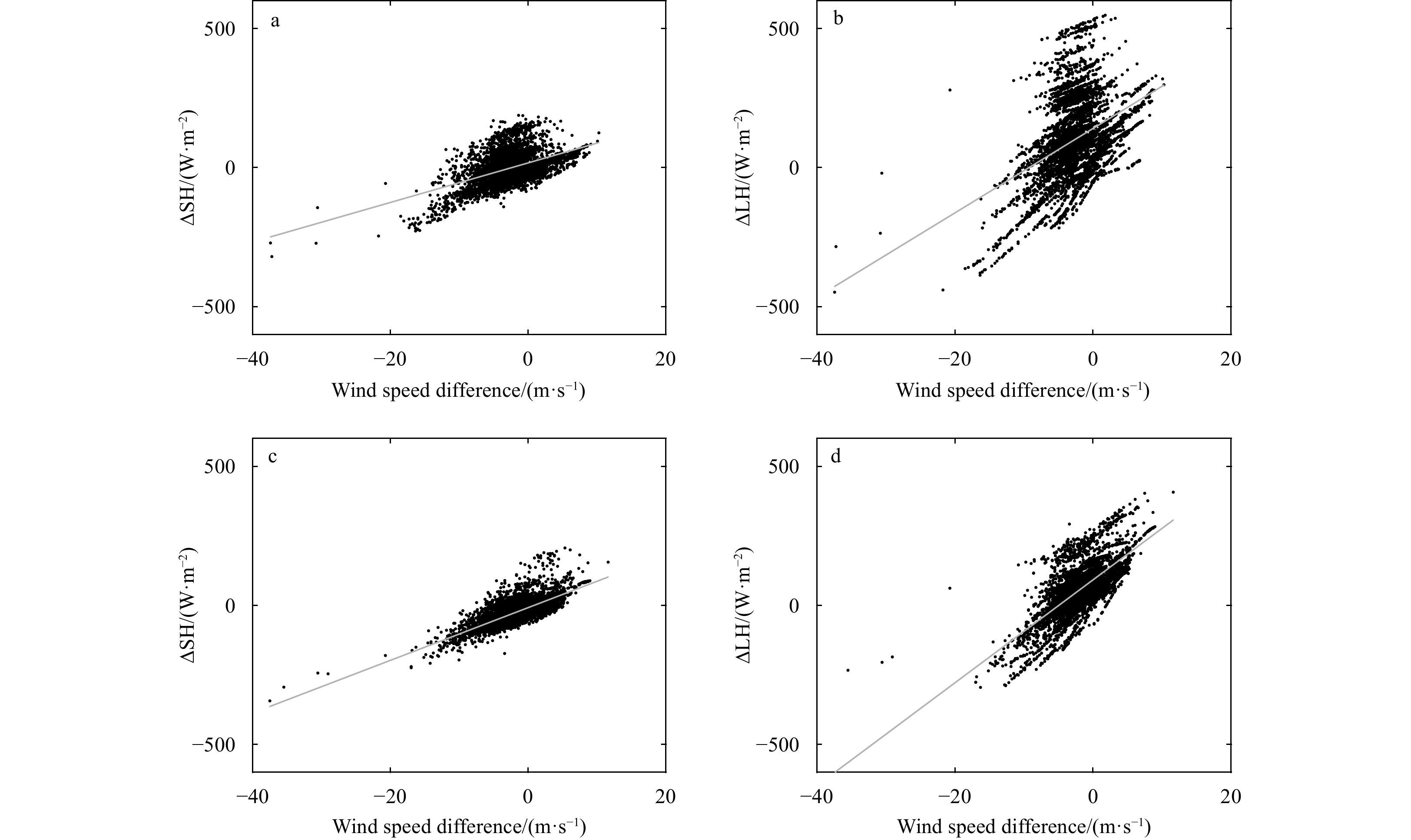
To better understand the impact of wind speed on the accuracy of NCEP and OAFlux products, the differences in wind speed and heat flux were compared (Fig. 9). The differences in wind speed between NCEP/OAFlux and the wave glider were denoted as ΔWNCEP-WG and ΔWOAFlux-WG, respectively. The absolute values of the correlation coefficients between ΔWNCEP-WG and ΔLHNCEP-WG, and between ΔWNCEP-WG and ΔSHNCEP-WG, were 0.48 and 0.40, respectively, while those between ΔWOAFlux-WG and ΔLHOAflux-WG and between ΔWOAFlux-WG and ΔSHOAFlux-WG were 0.74 and 0.69, respectively. Therefore, it is inferred that wind speed has a significant impact on the uncertainties in heat flux.
Figure
9.
Scatter plots of wind speed differences versus SHF differences between the NCEP and wave glider data (a), LHF differences between the NCEP and wave glider data (b), SHF differences between the OAFlux and wave glider data (c), and LHF differences between the OAFlux and wave glider data (d). The gray lines are regression lines.
A Black Pearl wave glider was used to measure the turbulent heat flux, including SHF and LHF, in the East China Sea and the Kuroshio region. The COARE 3.0 algorithm was used to estimate the in situ turbulent heat fluxes by using the air-sea parameters measured by the wave glider. The averaged latent heat LHF and SHF were 235 W/m2 and 134 W/m2, respectively. One striking feature was that the values in the Kuroshio were significant larger than those in the East China Sea. The average SHF was 118 W/m2 in the East China Sea and 160 W/m2 in the Kuroshio region. The average LHF was 180 W/m2 in the East China Sea, while that in the Kuroshio area was 324 W/m2.
The paper validated the feasibility of NCEP and OAFlux products in this region. It is found that the LHF and SHF obtained by OAFlux were closer to those measured by the wave glider than those obtained by NCEP. The maximum deviation occurred in the East China Sea area and the Kuroshio recirculation zone, with ΔSHOAFlux-WG >200 W/m2 and ΔLHOAFlux-WG >400 W/m2. This shows that the NCEP and OAFlux products have large errors in areas of complex circulation, while the wave glider has great potential for measuring the air-sea heat flux of complex circulation structures. High-frequency observations of wind speed are necessary to improve the accuracy of turbulent heat flux, and wave gliders have the potential to improve turbulent heat flux reanalysis products.
Acknowledgements
The Black Pearl wave glider was provided by Ocean University of China and Tiangong University. We thank the NECP (https://www.ncep.noaa.gov/) and OAFlux (https://oaflux.whoi.edu/) for providing data.
Barnier B. 1998. Forcing the ocean. In: Chassignet E P, Verron J, eds. Ocean Modeling and Parameterization. Dordrecht, the Netherlands: Springer, 45–80
[2]
Chavez F P, Sevadjian J, Wahl C, et al. 2018. Measurements of pCO2 and pH from an autonomous surface vehicle in a coastal upwelling system. Deep-Sea Research Part II: Topical Studies in Oceanography, 151: 137–146. doi: 10.1016/j.dsr2.2017.01.001
[3]
Chelton D B, Schlax M G, Samelson R M. 2011. Global observations of nonlinear mesoscale eddies. Progress in Oceanography, 91(2): 167–216. doi: 10.1016/j.pocean.2011.01.002
[4]
Daniel T, Manley J, Trenaman N. 2011. The wave glider: enabling a new approach to persistent ocean observation and research. Ocean Dynamics, 61(10): 1509–1520. doi: 10.1007/s10236-011-0408-5
[5]
Dufour C O, Griffies S M, de Souza G F, et al. 2015. Role of mesoscale eddies in cross-frontal transport of heat and biogeochemical tracers in the Southern Ocean. Journal of Physical Oceanography, 45(12): 3057–3081. doi: 10.1175/JPO-D-14-0240.1
[6]
Fairall C W, Bradley E F, Godfrey J S, et al. 1996. Cool-skin and warm-layer effects on sea surface temperature. Journal of Geophysical Research, 101(C1): 1295–1308. doi: 10.1029/95JC03190
[7]
Frenger I, Gruber N, Knutti R, et al. 2013. Imprint of Southern Ocean eddies on winds, clouds and rainfall. Nature Geoscience, 6(8): 608–612. doi: 10.1038/ngeo1863
[8]
Hine R, Willcox S, Hine G, et al. 2009. The wave glider: a wave-powered autonomous marine vehicle. In: Proceedings of OCEANS 2009. Biloxi, MS, USA: IEEE
[9]
Hogg A M C, Dewar W K, Berloff P, et al. 2009. The effects of mesoscale ocean–atmosphere coupling on the large-scale ocean circulation. Journal of Climate, 22(15): 4066–4082. doi: 10.1175/2009JCLI2629.1
[10]
Ko S H, Hyeon J W, Lee S, et al. 2018. Observation of surface water temperature and wave height along the coast of Pohang using wave gliders. Journal of Coastal Research, 85: 1211–1215. doi: 10.2112/SI85-243.1
[11]
Kubota M, Iwasaka N, Kizu S, et al. 2002. Japanese ocean flux data sets with use of remote sensing observations (J-OFURO). Journal of Oceanography, 58(1): 213–225. doi: 10.1023/A:1015845321836
[12]
Liu Jiping, Curry J A. 2006. Variability of the tropical and subtropical ocean surface latent heat flux during 1989−2000. Geophysical Research Letters, 33(5): L05706. doi: 10.1029/2005GL024809
[13]
Manley J, Willcox S. 2010. The wave glider: a persistent platform for ocean science. In: Proceedings of OCEANS’10 IEEE SYDNEY. Sydney, Australia: IEEE
[14]
Martin A J, Hines A, Bell M J. 2007. Data assimilation in the FOAM operational short-range ocean forecasting system: a description of the scheme and its impact. Quarterly Journal of the Royal Meteorological Society, 133(625): 981–995. doi: 10.1002/qj.74
[15]
Mitarai S, McWilliams J C. 2016. Wave glider observations of surface winds and currents in the core of Typhoon Danas. Geophysical Research Letters, 43(21): 11312–11319
[16]
Pagniello C M L S, Cimino M A, Terrill E. 2019. Mapping fish chorus distributions in southern California using an autonomous wave glider. Frontiers in Marine Science, 6: 526. doi: 10.3389/fmars.2019.00526
[17]
Penna N T, Maqueda M A M, Martin I, et al. 2018. Sea surface height measurement using a GNSS wave glider. Geophysical Research Letters, 45(11): 5609–5616. doi: 10.1029/2018GL077950
[18]
Pinardi N, Stander J, Legler D M, et al. 2019. The joint IOC (of UNESCO) and WMO collaborative effort for Met-Ocean services. Frontier in Marine Science, 6. doi: 10.3389/fmars.2019.00410
[19]
Schmidt K M, Swart S, Reason C, et al. 2017. Evaluation of satellite and reanalysis wind products with in situ wave glider wind observations in the Southern Ocean. Journal of Atmospheric and Oceanic Technology, 34(12): 2551–2568. doi: 10.1175/JTECH-D-17-0079.1
[20]
Smith N, Kessler W S, Cravatte S, et al. 2019. Tropical pacific observing system. Frontiers in Marine Science, 6: 31. doi: 10.3389/fmars.2019.00031
[21]
Sun Xiujun, Wang Lei, Sang Hongqiang. 2019. Application of wave glider “Black Pearl” to Typhoon Observation in South China Sea. Journal of Unmanned Undersea Systems (in Chinese), 27(5): 562–569
[22]
Sun Bomin, Yu Lisan, Weller R A. 2003. Comparisons of surface meteorology and turbulent heat fluxes over the Atlantic: NWP model analyses versus moored buoy observations. Journal of Climate, 16(4): 679–695. doi: 10.1175/1520-0442(2003)016<0679:COSMAT>2.0.CO;2
[23]
Thomson J, Girton J. 2017. Sustained measurements of Southern Ocean air−sea Coupling from a wave glider autonomous surface vehicle. Oceanography, 30(2): 104–109. doi: 10.5670/oceanog.2017.228
[24]
Ueyama R, Deser C. 2008. A climatology of diurnal and semidiurnal surface wind variations over the tropical Pacific Ocean based on the Tropical Atmosphere Ocean moored buoy array. Journal of Climate, 21(4): 593–607. doi: 10.1175/JCLI1666.1
[25]
van Lancker V, Baeye M. 2015. Wave glider monitoring of sediment transport and dredge plumes in a shallow marine sandbank environment. PLoS ONE, 10(6): e0128948. doi: 10.1371/journal.pone.0128948
[26]
Villareal T A, Wilson C. 2014. A comparison of the Pac-X Trans-Pacific wave glider data and satellite data (MODIS, Aquarius, TRMM and VIIRS). PLoS ONE, 9(3): e92280. doi: 10.1371/journal.pone.0092280
[27]
Wang Dongxiao, Zeng Lili, Li Xixi, et al. 2013. Validation of satellite-derived daily latent heat flux over the South China Sea, compared with observations and five products. Journal of Atmospheric and Oceanic Technology, 30(8): 1820–1832. doi: 10.1175/JTECH-D-12-00153.1
[28]
Waseda T, Mitsudera H, Taguchi B, et al. 2005. Significance of high-frequency wind forcing in modelling the Kuroshio. Journal of Oceanography, 61(3): 539–548. doi: 10.1007/s10872-005-0061-z
[29]
Yu Lisan, Weller R A. 2007. Objectively analyzed air–sea heat fluxes for the global ice-free oceans (1981−2005). Bulletin of the American Meteorological Society, 88(4): 527–540. doi: 10.1175/BAMS-88-4-527
[30]
Yusup Y, Liu Heping. 2020. Effects of persistent wind speeds on turbulent fluxes in the water–atmosphere interface. Theoretical and Applied Climatology, 140(1–2): 313–325
[31]
Zeng Lili, Wang Dongxiao. 2009. Intraseasonal variability of latent-heat flux in the South China Sea. Theoretical and Applied Climatology, 97(1–2): 53–64. doi: 10.1007/s00704-009-0131-z
[32]
Zhang Yanwu, Rueda C, Kieft B, et al. 2019. Autonomous tracking of an oceanic thermal front by a wave glider. Journal of Field Robotics, 36(5): 940–954. doi: 10.1002/rob.21862
Yuncong Jiang, Yubin Li, Yixiong Lu, et al. Evaluating nine different air-sea flux algorithms coupled with CAM6. Atmospheric Research, 2024. doi:10.1016/j.atmosres.2024.107486
2.
Hongqiang Sang, Jiangfan Ji, Xiujun Sun, et al. A path planning for formation rendezvous of the wave gliders considering ocean current disturbance. Ocean Engineering, 2024, 299: 117285. doi:10.1016/j.oceaneng.2024.117285
3.
Di Tian, Han Zhang, Shuai Wang, et al. Sea Surface Wind Structure in the Outer Region of Tropical Cyclones Observed by Wave Gliders. Journal of Geophysical Research: Atmospheres, 2023, 128(3) doi:10.1029/2022JD037235
4.
Hongqiang Sang, Zilu Zhang, Xiujun Sun, et al. Maneuverability prediction of the wave glider considering ocean currents. Ocean Engineering, 2023, 269: 113548. doi:10.1016/j.oceaneng.2022.113548
5.
Chunhua Qiu, Hong Liang, Xiujun Sun, et al. Extreme Sea-Surface Cooling Induced by Eddy Heat Advection During Tropical Cyclone in the North Western Pacific Ocean. Frontiers in Marine Science, 2021, 8 doi:10.3389/fmars.2021.726306
Huabin Mao, Xiujun Sun, Chunhua Qiu, Yusen Zhou, Hong Liang, Hongqiang Sang, Ying Zhou, Ying Chen. Validation of NCEP and OAFlux air-sea heat fluxes using observations from a Black Pearl wave glider[J]. Acta Oceanologica Sinica, 2021, 40(10): 167-175. doi: 10.1007/s13131-021-1816-0
Huabin Mao, Xiujun Sun, Chunhua Qiu, Yusen Zhou, Hong Liang, Hongqiang Sang, Ying Zhou, Ying Chen. Validation of NCEP and OAFlux air-sea heat fluxes using observations from a Black Pearl wave glider[J]. Acta Oceanologica Sinica, 2021, 40(10): 167-175. doi: 10.1007/s13131-021-1816-0
Figure 1. The Black Pearl wave glider (a) and wave glider path (b). The background data are OSTIA SST from January 30, 2019. The arrows indicate the locations of the wave glider for the corresponding date.
Figure 2. Scatter plots of wave glider SST and OSTIA SST (a) and wave glider wind speed and WindSat wind speed (b). The blue line is ${{{{y}}}}={{{{x}}}}$. The black dash line is the fitted line.
Figure 3. Spatial distribution of SHF (a) and LHF (b) observed by the Black Pearl wave glider.
Figure 4. Time series of SHF (a) and LHF (b). The NCEP, OAFlux, and wave glider values are represented by black, blue, and red lines, respectively.
Figure 5. Time series of differences in SHF (a) and LHF (b). The difference between the NCEP data and wave glider measurements is denoted by the black line, and that of OAFlux by the blue line.
Figure 6. Spatial distribution of differences in sensible heat flux (∆SH) between the NCEP and wave glider data (a), ∆SH between OAFlux and the wave glider (b), latent heat flux (∆LH) between NCEP and the wave glider (c), and ∆LH between OAFlux and the wave glider (d).
Figure 7. Display of time series of wind speed at 10 m (a), SST (b), and air temperature (c) during the measurements. The parameters derived from the NCEP, OAFlux, and wave glider data are black, blue, and red, respectively.
Figure 8. Display of time series of differences in wind speed at 10 m (a), SST (b), and air temperature (c) during the measurements. The difference between the NCEP and wave glider data is shown as a black line, and that between OAFlux and wave glider as a blue line.
Figure 9. Scatter plots of wind speed differences versus SHF differences between the NCEP and wave glider data (a), LHF differences between the NCEP and wave glider data (b), SHF differences between the OAFlux and wave glider data (c), and LHF differences between the OAFlux and wave glider data (d). The gray lines are regression lines.


 DownLoad:

 DownLoad:


 DownLoad: