Prediction of visibility in the Arctic based on dynamic Bayesian network analysis

1. Introduction

With the accelerated warming of the world, Arctic passages have received increasing attention because of melting ice. As the natural environment is complex and harsh in the Arctic, an objective assessment of the navigation risks for crossing the Arctic marine areas is urgently needed. The main factors that affect the navigation risk in the Arctic are sea ice and visibility (Vis) (Li et al., 2011; Gultepe et al., 2011, 2019). In general, sea-ice data are sufficient for risk assessment in the Arctic (data from satellite and meteorological model); however, observations of Vis are limited, leading to limited predictions (Gultepe et al., 2011, 2017). For this reason, improving Vis prediction is significantly important for safe navigation in the Arctic.

The Vis is the greatest horizontal distance at which it is possible to observe and identify particular objects. Currently, two methods can be used to predict Vis: (1) numerical weather prediction (NWP) models and (2) statistical prediction (SP) algorithms. NWP models are one of the most frequently used methods to predict Vis; however, the coarse spatial resolution of NWP models and their assumptions in the physical algorithms cannot accurately reflect real atmospheric processes (Gultepe et al., 2017). For example, it is assumed that Vis can be diagnosed from the liquid water content (LWC), droplet number concentration (Nd), and radar reflectivity parameter; at the same time, initial and boundary conditions are usually taken from large-scale or even global model simulations in numerical forecast models, which could result in severe problems for Vis prediction. Additionally, the products of microphysical parameterization schemes that are used in Vis prediction are very sophisticated and uncertainties always exist, leading to large uncertainties in the estimations of LWC and Nd (Gultepe et al., 2006; Gultepe and Isaac, 2006; Zhou et al., 2012).

With the development of marine transportation and artificial intelligence methods, the SP for Vis has become much more important in recent years. Pasini et al (2001), Bremnes and Michaelides (2007), as well as Marzban et al. (2007), applied neural network statistical analysis to predict Vis based on probabilistic concepts. They found that the performance of neural networks is generally superior to other methods in predicting Vis. Otto et al. (2007) used subjective and objective analysis techniques to predict Vis. Their results showed that the combination of the above two analyses can be used to construct climatological guidelines for forecasters. Boneh et al. (2015) also developed an SP technique called the Bayesian decision network for fog prediction, which had a better performance than historical operational skill indices. Although the above studies improved the accuracy of SP for Vis, they did not fully reduce the uncertainty in the prediction of Vis, suggesting that more work is needed in this area. Two aspects should be improved in future work, one is the network structure of SP for calculating Vis and the other is the ability of SP to deal with time-series information for improving the robustness of the predicted results.

Earlier efforts have been made to improve Vis predictions by integrating NWP model outputs with SP analysis data. Roquelaure and Bergot (2008, 2009), Roquelaure et al. (2009), and Chmielecki and Raftery (2011) applied Bayesian models to average Vis predictions, thereby improving ensemble predictions including underestimation and discrepancies in predictions. Similarly, Zhou et al. (2012) made an effort to improve Vis prediction in three aspects: (1) the application of a rule-based fog detection scheme, (2) the extension of the National Centres for Environmental Prediction Short Range Ensemble Forecast System to fog Vis ensemble probabilistic predictions, and (3) a combination of these two applications. As uncertainties always exist in model physics and such uncertainties vary for different times, locations, and cases (Zhou et al., 2012), many studies still need to be performed to improve Vis prediction.

Presently, Vis prediction is very limited (Gultepe et al., 2006, 2009) and it is necessary to improve the accuracy of the predicted Vis to ensure the safety of shipping activities in the Arctic. As the dynamic Bayesian network (DBN) has a solid mathematical basis in probability theory and has been widely used to reduce uncertainties in calculated results (Li and Liu, 2018), Vis prediction based on DBN can be feasible even though the scales used are still large compared to many fog events. At the same time, the DBN combines both historical information and up-to-date evidence of predictors to predict Vis. This guarantees that the DBN model can not only learn the statistical characteristics of historical Vis but also leverage the latest changes in Vis to predict future Vis. Therefore, predicting Vis based on DBN is theoretically feasible. As both historical continuous observed data of Vis and its influence factors are necessary to train the DBN parameters, this study uses the artificial neural network (ANN) and reanalysis data from European Centre for Medium-Range Weather Forecasts (ECMWF) to reconstruct historical gridded Vis in the Arctic areas. Then, the predicted Vis based on DBN is provided, showing that DBN is a feasible and accurate method to predict Vis compared to previous analysis methods.

The objectives of this study are twofold: (1) to generate reliable historical continuous gridded data of Vis in the Arctic, and (2) to test the feasibility of DBN when predicting Vis in the Arctic. The remainder of this paper is organised as follows. Section 2 called project requirements is provided for clarifying data analysis and observations. Section 3 describes the DBN. Section 4 presents the results of this study. The final section (Section 5) provides the discussion and conclusions.

2. Project requirements

2.1 Factors affecting Vis

Many factors influence Vis predictions, such as hydrometeors of aerosols, fog, rain, and snow, as well as meteorological elements such as relative humidity (RH), air temperature (Ta), and horizontal wind speed (Uh) (Gultepe et al., 2019). Meteorological elements have a direct influence on sea fog and precipitation; these two weather phenomena are considered to be the main events affecting Vis. The current work considers only meteorological elements when calculating Vis using ANN and DBN. Many previous studies have revealed the relationship between Vis and other meteorological elements. Xue et al. (2015) studied the effects of air pollution and meteorological elements on Vis in Shanghai, China. Their results showed that Ta and Uh were positively correlated with Vis, whereas RH was negatively correlated with it. Hong (2003) also studied the relationship between Vis and its influence factors based on binary correlation and partial correlation methods. Their results showed that RH and rainfall precipitation rate were negatively correlated with Vis, while Ta and Uh were positively correlated. Gultepe et al. (2017) showed that an increasing Ta may result in better Vis conditions, and a decreasing Uh with increasing RH may lead to low Vis values.

As precipitation and sea fog are the main weather phenomena influencing Vis in the Arctic regions (Gultepe et al., 2015), the factors influencing precipitation and sea fog occurrence should also be considered in the analysis. Zhao et al. (2012) studied the relationship between pressure and rainfall in East Asia. Furthermore, Kutiel et al. (2001) studied the changes in sea surface pressure (Ps) with rainfall conditions and found that the pressure field was closely related to rainfall intensity. These findings are evidently because frontal precipitation systems are related to strong changes in thermodynamic and dynamic conditions. Qu et al. (2014) performed a detailed statistical analysis of sea fog in Bohai Bay and discussed its formation mechanism. Their results suggested that the optimal wind speed during fog events in Bohai Bay was from 1.6 m/s to 5.4 m/s, indicating the importance of wind and turbulence intensity on fog conditions. Most (88%) of their fog cases met the advective marine fog conditions when the sea surface temperature (Ts) was higher than Ta. In summary, RH, Ts, Ta at 10 m, Uh, Ps, and the temperature difference between sea and air temperatures (TDsa) were considered for Vis prediction based on DBN.

2.2 Data

The data used to train the ANN were obtained from the International Comprehensive Ocean-Atmosphere Data Set (ICOADS). Data used to generate daily gridded Vis products at 12:00 UTC in the Arctic were obtained from the ECMWF. The influence factors of Vis in the analysis include RH, Ts, Ta, Uh, Ps, and TDsa (Section 2.1). To test the accuracy of the generated gridded daily Vis products based on ANN, Vis observations from the Chinese 9th Arctic Science Expedition (CNASE) field project were used in this study. Information on these datasets is provided in the following subsections.

2.2.1   International Comprehensive Ocean-Atmosphere Data Set

The ICOADS archives (Freeman et al., 2017) are the largest collection of ocean surface observational data sets with observations from 1784 to the present, which includes data from ships, buoys, and coastal sites located all over the world. These datasets are distributed by the National Climate Information Centre (NCIC) of the United States. Owing to the sampling nature, the station number density in a specific area changes with time and location. The ICOADS data used in this study include Vis, RH, Ts, Ta, Uh, Ps, and TDsa in the Arctic from 2000 to 2014. Vis records come with a Vis level, as described in the ICOADS documents (Table 1), as well as by Gultepe et al. (2019).

Table  1.  Rules of classifying visibility (Vis) levels

Vis level	Vis interval/km	Vis/km
1	0.05	≤0.05
2	0.15	0.05–0.20
3	0.3	0.2–0.5
4	0.5	0.5–1.0
5	1	1–2
6	2	2–4
7	6	4–10
8	10	10–20
9	30	20–50
10	−	≥50
Note: − represents no data.

 | Show Table

DownLoad: CSV

As a large amount of poor quality data exists in the ICOADS archives, it is necessary to pre-process the data before using it in the analysis, which includes eliminating incomplete records and data of poor quality. Each datapoint has its own quality flag (QF) in the ICOADS archives, and different QFs represent the different qualities of these data (Table 2). In the analysis, data of good quality (QF 1, element appears correct) were used in this study.

Table  2.  Quality flag (QF) of data records from the International Comprehensive Ocean-Atmosphere Data Set

QF	Description of QF
0	no quality control performed
1	element appears correct
2	element appears inconsistent with other elements
3	element appears doubtful
4	element appears erroneous
5	element changed (possibly to missing) as a result of quality control
6	element flagged by contributing member (CM) as correct but according to minimum quality control standard (MQCS) still appears suspect or missing
7	element flagged by CM as changed, but according to MQCS still appears suspect
8	reserved
9	element is missing

 | Show Table

DownLoad: CSV

2.2.2   The Chinese 9th Arctic Science Expedition

The observations used to test the accuracy of the generated gridded Vis products from the ANN were obtained from CNASE, which represents the period of July 20–September 26, 2018. The scientific expedition covered more than 12.5×10⁶ n mile, including 3 815 n mile of ice-covered areas. The northernmost latitude of the expedition was 84.8°N. The navigation trajectory of the CNASE is shown in Fig. 1. The data recorded in this experiment included both meteorological and marine observational data. The meteorological data included Ta, RH, Ps, Uh, horizontal Vis, cloud cover, and cloud base height. The marine data included Ts, salinity, fluorescence, and coloured dissolved organic matter.

Figure  1.  Navigation trajectory of the ice breaker ship used during the Chinese 9th Arctic Science Expedition from July 20 to September 26, 2018.

DownLoad: Full-Size Img PowerPoint

2.2.3   ERA-Interim data

The ECMWF-Reanalysis Archive (ERA) Interim data (Dee et al., 2011) are the gridded data product distributed by the ECMWF, which includes both observations and predicted products for the entire world, and these data are used for NWP model initialization during the next prediction hours. The ERA-Interim data is the 3rd level generation product and its quality is significantly higher than that of the 2nd level generation product, ERA-40. These data represent the period from 1979 to the present and are constantly updated. The dataset has a variety of temporal and spatial resolution products, of which the minimum (maximum) temporal resolution is 3 h (1 month). The minimum (maximum) grid resolution is 0.125°×0.125° (3°×3°).

3. Methods and model

3.1 Technology route

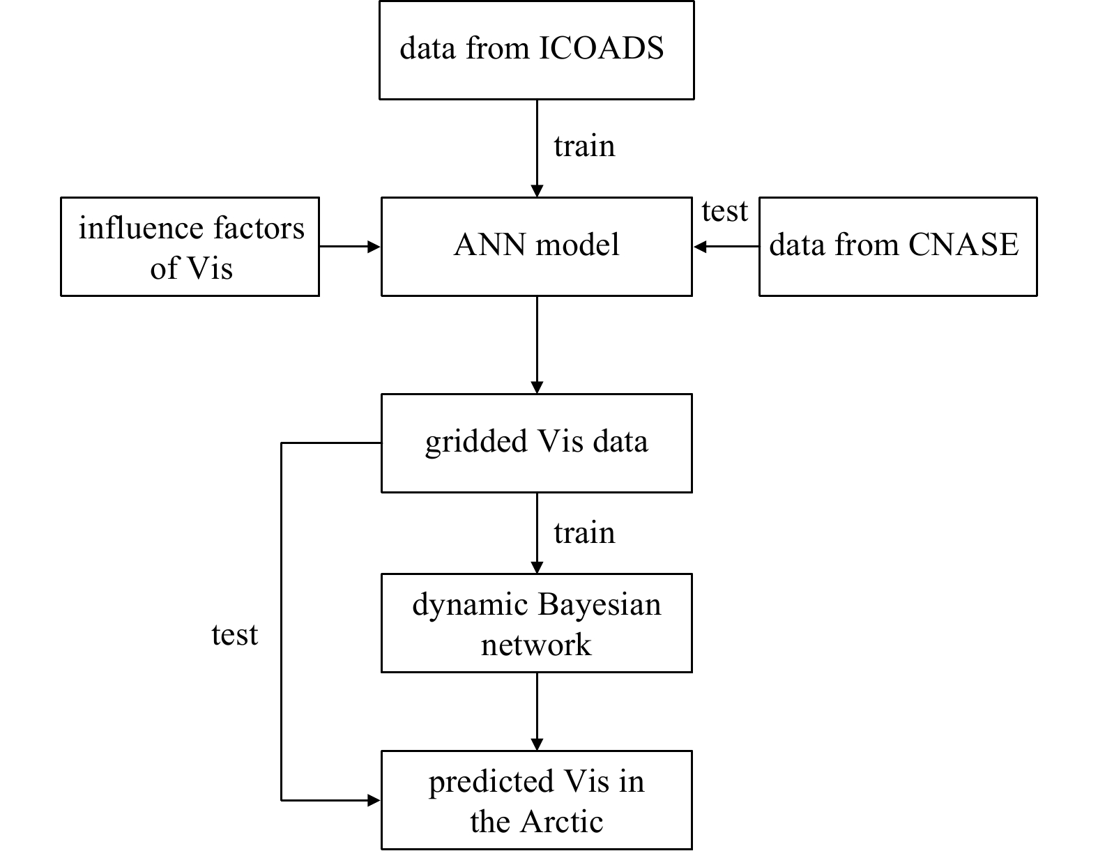
The technical route studied in this study is shown in Fig. 2. First, the influence factors of Vis were screened according to the previous sections. Then, the structure of the DBN to predict Vis was built based on the screened factors. Subsequently, the DBN parameters were trained with the training datasets. Three experiments for predicting Vis were carried out in the Arctic covering an area from 70°–90°N. Finally, the validity of the DBN model was verified by the three experiments for predicting Vis in the Arctic. Owing to the paucity of historical and continuous Vis data used to train the DBN parameters, this study generated historical and continuous daily gridded Vis data with an ANN model. The accuracy of the generated Vis data based on the ANN was also verified against the observed Arctic data from CNASE. The parameters of the ANN were trained using datasets from ICOADS.

Figure  2.  Flow chart of dynamic Bayesian network analysis in this paper.

DownLoad: Full-Size Img PowerPoint

3.2 Artificial neural network

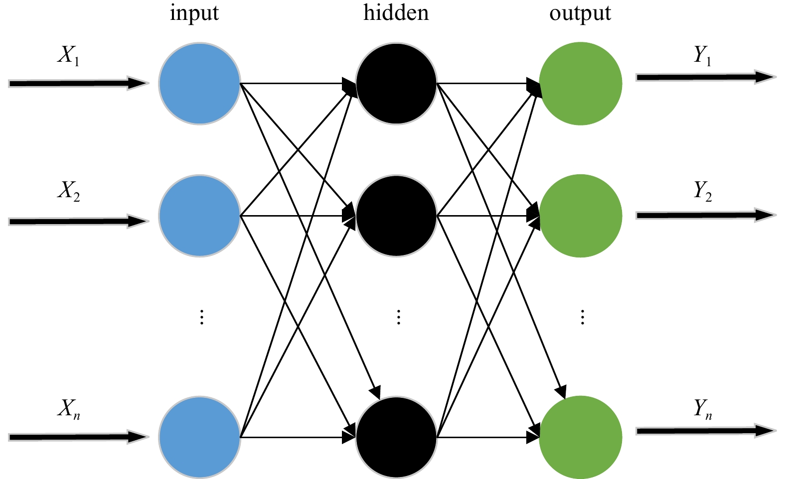
ANN have been studied since the 1940s and have been widely applied in the military, medical science, and broader economy. This paper employs a backpropagation (BP) network to infer Vis data, which was first proposed by McClelland et al. (1987) in 1986. The BP network is a classical ANN that can simulate any nonlinear input–output relationship.

There are three layers in a BP network: the input, hidden, and output layers. The neurons are connected with others in the adjacent layers but the neurons in the same layer are not connected. The input and output layers comprise a single layer but the hidden layer can have a different number of layers, and the number of neurons in each layer is also different depending on the layer properties. The structure of the BP network topology with only one hidden layer is shown in Fig. 3.

Figure  3.  Topological structure of the backpropagation network, which includes only one layer of the hidden layer.

DownLoad: Full-Size Img PowerPoint

The signal in the ANN was transmitted from the input layer to the output layer. The output value of each node in the hidden layer depends on the input value, the weight of each node in the input layer that influences the node value in the hidden layer, and the threshold value and activation function of each node in the hidden layer.

where $ {X}_{j}^{'} $ is the output value of the jth neuron in the hidden layer when a value is input, $ {\omega }_{ij} $ is the weight at which the ith value in the input layer influences the jth value in the hidden layer, $ {X}_{i} $ is the ith value in the input vector, $ {\theta }_{j} $ is the threshold of the jth neuron in the hidden layer, and f is the activation function of the jth neuron in the hidden layer. The signal transmission rule between the input and hidden layers is the same as that between the hidden layer and the output layer.

The ANN model constructed in this study was trained based on BP algorithm (Jin et al., 2000). When there is an error between the actual output value and the ideal output value, the error is transmitted from the output layer to the hidden layer and input layer to amend the weight and threshold of each neuron. The training process was completed only when the error was less than the convergence threshold. ANN technology is highly suitable for simulating the nonlinear relationship between Vis and its influence factors. Therefore, gridded Vis can be calculated based on an ANN when the data of its influence factors are known.

3.3 Dynamic Bayesian network

A Bayesian network (Pearl, 1988) is a directed and acyclic graph system, whose nodes represent the random variables considered in the problem of Vis prediction. Directed arcs connect pairs of nodes, representing direct dependencies (which are often causal connections) between variables. A line from the Y_i to Y_j depicts the dependence between the two variables. A simple interpretation of this connection is that variable Y_i has an impact on Y_j, and Y_i is taken as the parent nodes of Y_j. The relationship between variables is quantified by conditional probability distributions associated with each node, where the state of the child nodes depends on the combination of the values of parent nodes. The Bayesian Network (BN) is obtained using Bayes’ theory, which is expressed as

where $ P(X|Y) $ is the probability of occurrence for $ X $ based on the occurrence for $ Y $. $ P\left(X\right) $, $ P\left(Y\right) $, and $ P(Y|X) $ are the probability of occurrence for $ X $, $ Y $ and $ Y $ based on occurrence for $ X $, respectively.

For a BN with nodes $ {X}_{1},\;{X}_{2},\;\dots ,{X}_{n} $, the joint distribution function is expressed as

where $ {\rm{Parents}}\left({X}_{i}\right) $ represents the parent nodes of $ {X}_{i} $.

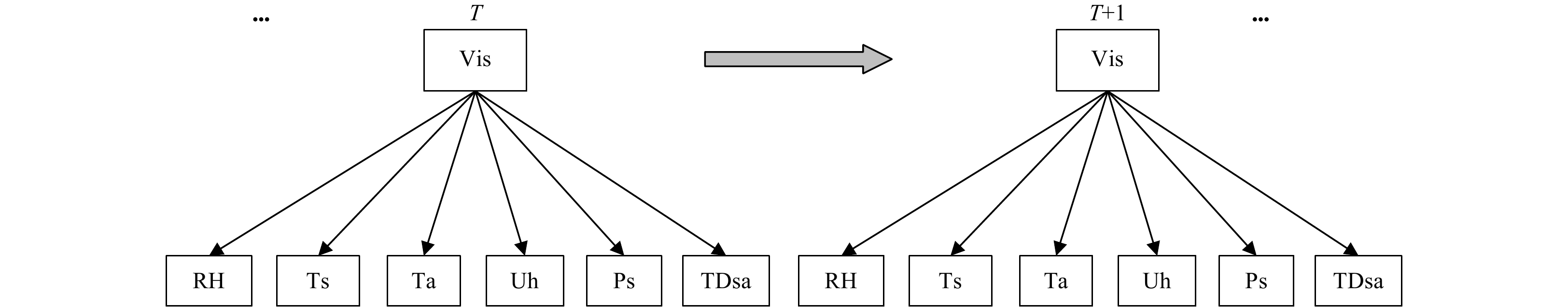
The DBN is a system model based on a hidden Markov Model and static BN, which introduces the time dimension into the traditional static BN theory to describe the change and evolution of the system over time (Shi and Zhang, 2012). The nodes of the DBN include both hidden and observable variable nodes, where the hidden variable is unobservable and needs to be calculated. The principle of a DBN with one observable variable and one hidden variable is as follows:

where $ X=\left\{{x}_{0},{x}_{1},\dots ,{x}_{T-1}\right\} $ represents a sequence of hidden variables, $ Y=\left\{{y}_{0},{y}_{1},\dots ,{y}_{T-1}\right\} $ represents a sequence of observable variables, and T is the time limit of the studied event.

Three parameter sets need to be defined to describe DBN: (1) the state transition probability distribution function (STPDF), $ P\left({x}_{t}|{x}_{t-1}\right), $ which is defined to describe the change of one node with time and can guarantee the stability of the calculated result. Note that the state transition probability matrix (STPM) between adjacent time slices does not change. (2) The probability distribution function of the observation node $ P\left({y}_{t}|{x}_{t}\right), $ which describes the relationship between hidden nodes and observable nodes in time slice t, and (3) the initial state distribution function $ P\left({X}_{0}\right) $, which describes the initial state.

The learning of the DBN is an extension of a traditional BN, including parameter learning and graph structure learning. Parameter learning refers to learning conditional probability tables (CPTs) from sample data, which include the CPT of the hidden and observable nodes and STPDF. Graph structure learning refers to learning a BN structure from sample data that can better reflect the causal relationship of nodes. As the result of the DBN graph structure learning is still a static DBN structure (similar to the structure learning of a traditional BN), this paper does not introduce a new structure learning based on the DBN. According to the integrity of the sample data and the known structure, DBN learning can be divided into the four situations given in Table 3. As the DBN structure has been determined a priori, the method used to train the DBN parameters here is the Expectation-Maximization (EM) algorithm.

Table  3.  Summary of automatic learning methods used in dynamic Bayesian network

The known of structure	The integrity of sample data	Automatic learning methods
known	complete	simple statistical method
known	incomplete	EM method or gradient descent method
unknown	complete	searching model space
unknown	incomplete	structural EM method

 | Show Table

DownLoad: CSV

The structure of the DBN used to predict Vis is shown in Fig. 4. From Eq. (4) and Fig. 4, we know that

Figure  4.  Structure of dynamic Bayesian network to predict visibility (Vis).

DownLoad: Full-Size Img PowerPoint

representing a sequence of hidden variables;

representing a sequence of observable variables. Therefore,

where $ {y}_{11} $=$ {{\rm{RH}}}_{0} $, $ {y}_{21} $=$ {{\rm{Ts}}}_{0} $, $ {y}_{31} $=$ {{\rm{Ta}}}_{0} $, $ {y}_{41} $=$ {{\rm{Uh}}}_{0} $, $ {y}_{51} $=$ {{\rm{Ps}}}_{0} $, and $ {y}_{61} $=$ {{\rm{TDsa}}}_{0} $. As the data processed in the DBN are discrete, it is necessary to discretize the data before inputting them to the DBN. The rule discretizing the Vis data is shown in Table 1. The rules discretizing RH, Ts, Ta, Uh, Ps, and TDsa are based on a uniform discretization principle and the range of each data is determined based on the historical data of these meteorological elements. The details of the discretization principle can be found in the supplementary materials.

4. Results

4.1 Performance of ANN analysis

Based on the trained BP neural network (MATLAB toolbox) and gridded daily reanalysis data from the ECMWF (representing Arctic areas for the period of 2008–2018), newly gridded daily Vis products were obtained at 12:00 UTC for each day on 0.5°×0.5° grid areas.

The BP neural network with three layers was first constructed, where the number of hidden layer node was five, the maximum number of iterations was 100, the learning rate was 0.1, and the convergence threshold was 0.000 01. Data from ICOADS in the Arctic were used to train the parameters of the constructed ANN and data from CNASE were used to test the effectiveness of the trained ANN method. Considering that Vis changes with monthly weather features, using the multi-year data of a specific month as a training sample to infer Vis in that month has a higher accuracy (Shan et al., 2019) compared to Vis inferred from other time periods using ANN. As inherent instability always exists in the ANN, an average of 30 experiments are used to finalise the inferred Vis. The number of data points from CNASE for each month is shown in Table 4.

Table  4.  Number of data points for each month in the Arctic obtained from the Chinese 9th Arctic Science Expedition archive

	July	August	September
Amount	73	355	201

 | Show Table

DownLoad: CSV

To assess the uncertainty of the inferred and predicted Vis, the relative error of Vis is defined as follows:

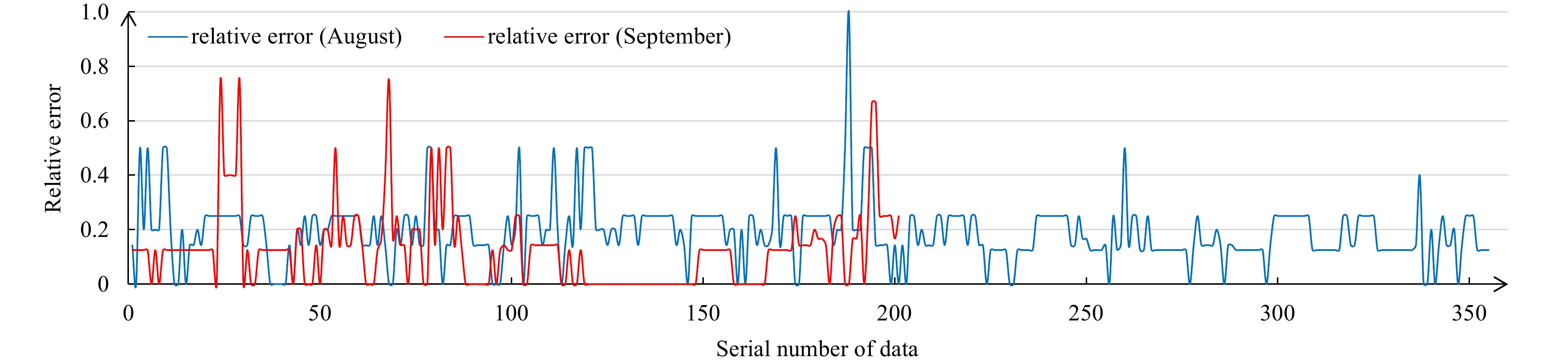
where $\text{δ} $ is the relative error; $ {{\rm{Vis}}}_{i} $ is either inferred or predicted Vis; and $ {{\rm{Vis}}}_{m} $ is the observed Vis. As the number of observed datapoints from CNASE in July was relatively small, the $\text{δ} $ of Vis from ANN was obtained only for the months of August and September; the results are shown in Fig. 5.

Figure  5.  Relative error (δ) of inferred Vis from Eq. (6) against observations obtained from the Chinese 9th Arctic Science Expedition.

DownLoad: Full-Size Img PowerPoint

Results suggested that average relative error values of all Vis from ANN for August and September are 19.0% and 12.7%, respectively. This suggested that the BP neural network could well simulate the nonlinear relationship between Vis and its influence factors. However, some inferred Vis values have a large relative error, which could be due to (1) the inadequate training of the neural networks or (2) the deficiency of the selected factors that influence Vis in the ANN model. The results also suggest that a better training algorithm for ANN and longer-term observations with high accuracy are needed to improve the inferred gridded Vis.

4.2 Performance of DBN

The generated historical continuous gridded data for the period of 2008–2017 in the Arctic were used to train the parameters of the constructed DBN model, while gridded data from 2018 were used to test the accuracy of the predicted Vis. The STPM of the DBN based on the training data and the EM algorithm is shown in Table 5. Note that the STPM does not change in the following three experiments for predicting Vis in the Arctic.

Table  5.  State transition probability matrix of the trained dynamic Bayesian network, where 1–10 represent the Vis level (state)

Vis	1	2	3	4	5	6	7	8	9	10
1	0.330	0.221	0.167	0.143	0.072	0.034	0.032	0.000	0.000	0.000
2	0.297	0.175	0.118	0.143	0.145	0.055	0.060	0.007	0.000	0.000
3	0.144	0.107	0.133	0.197	0.175	0.176	0.051	0.017	0.000	0.000
4	0.010	0.014	0.029	0.267	0.315	0.270	0.078	0.016	0.000	0.000
5	0.001	0.001	0.004	0.036	0.351	0.434	0.153	0.018	0.000	0.000
6	0.000	0.000	0.001	0.006	0.075	0.564	0.331	0.023	0.000	0.000
7	0.000	0.000	0.000	0.001	0.012	0.137	0.791	0.057	0.001	0.000
8	0.000	0.000	0.000	0.001	0.013	0.091	0.423	0.459	0.012	0.001
9	0.000	0.000	0.000	0.000	0.003	0.062	0.320	0.325	0.277	0.012
10	0.000	0.000	0.001	0.003	0.003	0.257	0.140	0.188	0.288	0.121

 | Show Table

DownLoad: CSV

Based on the trained DBN model, three prediction experiments were performed to test the feasibility of the DBN when predicting Vis in the Arctic. The first two experiments were conducted to predict Vis in the eastern part of the Arctic region, while the 3rd experiment was used to predict Vis in the entire Arctic region, where the time period of the predicted Vis is 5 d. As the result of DBN is the probability distribution of Vis at different levels, the Vis level with the maximum probability is taken as the final result of the DBN. The periods of the evidence data input in the three experiments were 10 d, 21 d, and 21 d, respectively. The prediction area of the first two experiments is the same, while the time period of the evidence data is different. Therefore, they could be used to study the effect of the time period of the evidence data on the predicted Vis. Similarly, the last two experiments could be used to study the effect of the size of the prediction area on the predicted Vis.

4.2.1   Results in the eastern part of Arctic region with 10 days’ evidence data

Data from January 1 to 10, 2019 were input into the trained DBN model to predict the daily Vis data in the eastern part of the Arctic region at 12:00 UTC from January 11 to 15, 2019. The predicted Vis from the DBN and inferred Vis (regarded as observed Vis) from the ANN, from January 11 to 15, 2019 are shown in Fig. 6. The results showed that the predicted Vis in the first three days was reasonable compared to observations but the results from day 4 were significantly different compared to the reference observed values. With the extension of the prediction period, the Vis values in the entire sea region tend to be the same. This is because the predicted result from the DBN is related to the STPM, which only depends on the sample data used to train the DBN model. The predicted Vis from January 11 to 13, 2019 showed that the DBN can well predict the coverage of sea regions with low Vis conditions (see the region within the red circle in Fig. 6); however, the accuracy of the predicted coverage for low Vis decreases with an increase in the prediction time (see the region within the blue circle in Fig. 6). This can be due to the invariance of the STPM when predicting future Vis using the DBN. Note that low Vis is typically defined as below 3 n miles (Xu, 2016); therefore, a Vis level below 6 was defined as low Vis in this paper. At the same time, a Vis level above 8 was defined as high Vis.

Figure  6.  Predicted visibility (Vis) from dynamic Bayesian network and inferred Vis from artificial netural network, for January 11–15, 2019, are shown in boxes a–e and f–j, respectively. The areas with good consistency for the coverage of low Vis between predicted Vis and inferred Vis are marked with red circles, while the areas with bad consistency for this coverage are marked with blue circles.

DownLoad: Full-Size Img PowerPoint

4.2.2   Results in the eastern part of Arctic region with 21 days’ evidence data

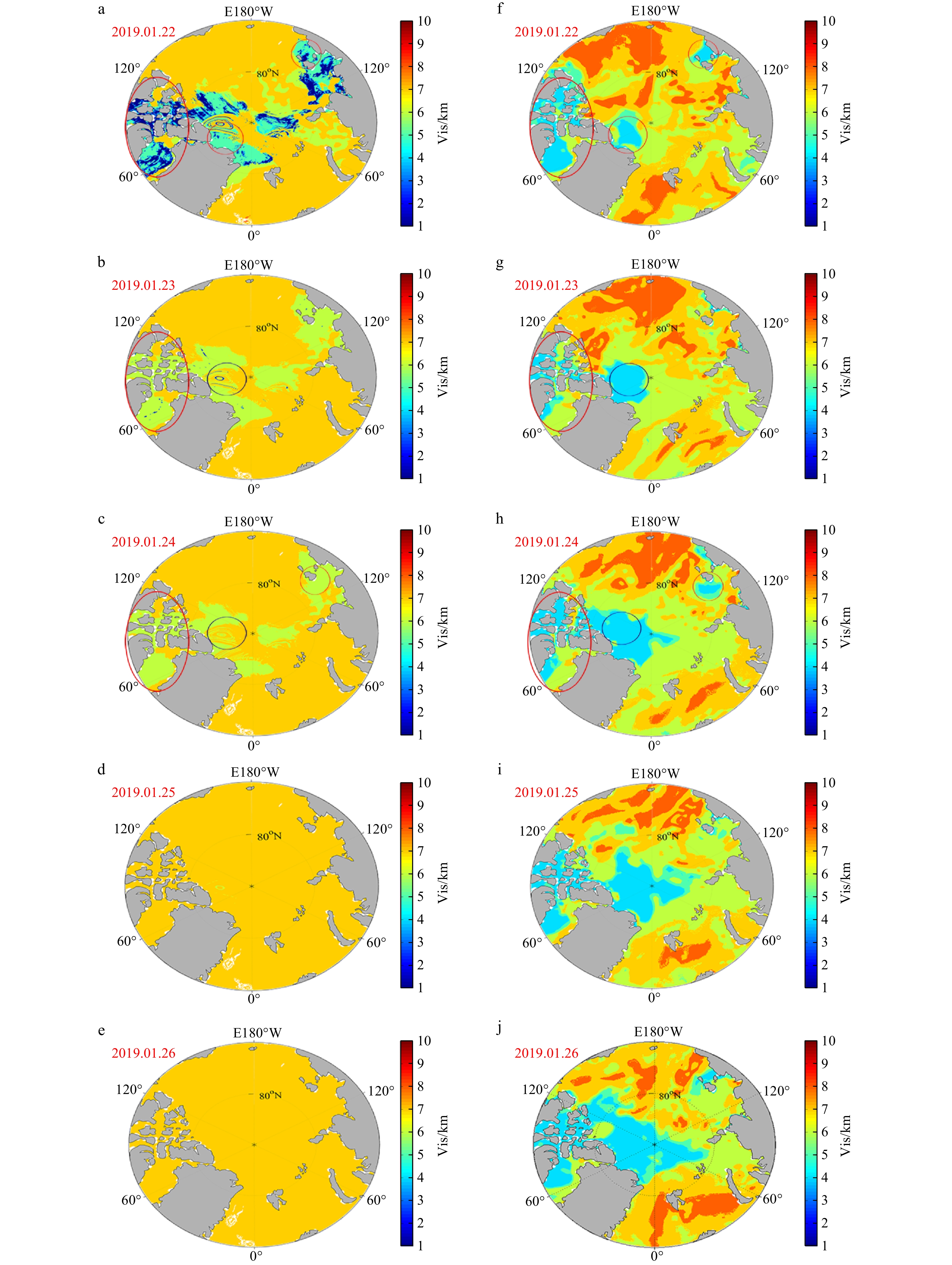
Data from January 1 to 21, 2019 were input into the trained DBN model to predict the daily Vis data in the eastern part of the Arctic region at 12:00 UTC from January 22 to 26, 2019. The predicted Vis from the DBN and inferred Vis (regarded as observed Vis) from the ANN, from January 22 to 26, 2019 are shown in Fig. 7. A similar conclusion can be obtained from the predicted results from January 22 to 26, 2019. At the same time, the DBN cannot accurately predict the coverage of sea regions with high Vis conditions (see the region within the blue circle in Figs 7a and f), which could be due to incomplete coverage of the sample data used to train the DBN. It was noticed that the DBN can predict Vis but only for 3 d, which also indicates that the accuracy of the predicted results decreases with time.

Figure  7.  Predicted visibility (Vis) from dynamic Bayesian network and inferred Vis from artificial netural network for January 22–26, 2019, are shown in boxes a–e and f–j, respectively. The areas with good consistency for the coverage of low Vis between the predicted Vis and inferred Vis are marked with red circles, while the areas with bad consistency for this coverage are marked with blue circles.

DownLoad: Full-Size Img PowerPoint

4.2.3   Results in the whole part of Arctic region with 21 days’ evidence data

To further test the accuracy of the results shown in Figs 6 and 7, data from January 1 to 21, 2019 were input into the trained DBN model to predict the daily Vis data over the entire Arctic sea area at 12:00 UTC for January 22–26, 2019 (Fig. 8). The results showed that DBN can generally well predict the coverage of the sea regions with low Vis values on January 22, 2019 (red circle in Fig. 8). However, the sea regions with low Vis conditions cannot be predicted well for both January 23 and 24, 2019. In addition, the result suggested that the predicted Vis in the first three days was reliable when compared to the prediction of day 4 and later. These results are consistent with previous results shown in Figs 6 and 7.

Figure  8.  Predicted visibility (Vis) from dynamic Bayesian network and inferred Vis from artificial netural network are shown in boxes a–e and f–j, respectively, for the period of January 22–26, 2019. The areas with good consistency for the coverage of low Vis between the predicted and inferred Vis are marked with red circles, while the areas with bad consistency for this coverage are marked with blue circles.

DownLoad: Full-Size Img PowerPoint

4.2.4   Analysis of the above three prediction experiments

Figure 9 shows the mean relative error of the daily predicted results relative to the inferred values from the ANN. As the predicted results from day 4 were unreliable, only the results from the first 3 days were worth further study. The mean relative error of predicted Vis over 3 days from January 11 to 13, 2019 was estimated to be 15.6%, while for the period of January 22–24, 2019 it was found to be 9% and 19.2%. This shows that the relative error of the predicted Vis results for these days is acceptable. At the same time, for the same prediction region and STPM, the accuracy of the predicted Vis is positively correlated with the time period of the input data. In addition, an increase in the prediction region increases the uncertainty of the predicted results.

Figure  9.  The mean relative error of the daily predicted results relative to the inferred Vis from artificial netural network.

DownLoad: Full-Size Img PowerPoint

It was also noticed that the predicted result on January 11, 2019 has a large relative error of 30.3%, as the predicted result from the DBN magnifies the incorrect degree of Vis (Fig. 6a). It can be concluded that although the DBN can predict Vis in areas with poor Vis, the model could also exaggerate the degree of poor Vis. Therefore, the distribution trend of the Vis predicted from the DBN could play a referential role for decision makers. Figure 9 also shows that the relative errors of the predicted Vis for the period of January 14–15, 2019 were found to be below 10%. However, the predicted results for these days are unreliable. Note that the predicted Vis on these days does not change significantly with time, which indicates that predictions of more than 3 days can be questionable. The relative error here is the error of the predicted Vis relative to Vis from the ANN, which could be accidental.

The prediction success rate (PSR) can also accurately reflect the accuracy of the predicted result. PSR is the proportion of grid points with an accurate prediction in the total grid points. Table 6 lists the daily PSRs of the three experiments. As the first 3 days of Vis predictions are reasonable compared to observations, this study only analysed the PSR in the first 3 days.

Table  6.  Daily prediction success rate of the three prediction experiments

	Day 1	Day 2	Day 3	Day 4	Day 5	Average of the first 3 days
Experiment 1	33.1%	51.4%	55.6%	58.5%	58.7%	46.7%
Experiment 2	59.8%	73.9%	46.9%	42.3%	38.1%	60.2%
Experiment 3	33.8%	42.8%	29.9%	23.2%	27.5%	35.5%

 | Show Table

DownLoad: CSV

It can be seen from Table 6 that the experiment for predicting Vis in the eastern part of the Arctic region with 21 days’ evidence data had the highest PSR at 60.2%. The experiment for predicting Vis in the entire Arctic region with 21 days’ evidence data had the lowest PSR at 35.5% and the PSR of the second experiment was 46.7%. The result confirms the conclusion that the uncertainty of the predicted Vis increases with the prediction area and time, while the accuracy of the predicted Vis has a positive correlation with the time period of the input evidence data.

5. Discussion and conclusions

This work generated continuous and historical gridded Vis data in the Arctic region based on ANN, and tested the feasibility of using a DBN to predict Vis. Three experiments were performed for predicting Vis over the Arctic Ocean region based on the trained DBN model. The prediction regions for the first two experiments was the eastern part of the Arctic region, while the third experiment was for the entire Arctic region. Overall, the following conclusions can be drawn from this work, which should be considered for future analysis.

(1) The BP neural network could well fit the relationship between Vis and its influence factors, and the average relative error of the inferred Vis from ANN was below 20%.

(2) The average relative error of the predicted Vis on the first 3 days from the three prediction experiments was found to be 14.6%. As the error of predicted Vis from NWP can easily reach more than 30% (Gultepe et al., 2006, 2009), the predicted Vis from DBN can be considered as more reliable.

(3) The DBN model constructed in this study could accurately predict the coverage of the sea regions with low Vis values, which meets the need to ensure the safety of sea navigation.

(4) The relative error of the predicted Vis from the DBN can reach 30% when predicting the Vis in the eastern part of Arctic region with 10 days’ evidence data, which indicates that meteorological observations with high quality to better train the parameters of DBN can improve the results of this study.

Interestingly, the DBN could predict Vis for only 3 days; in general, the predictive capability for Vis was relatively limited. This phenomenon could be because the STPM does not change when predicting Vis in the following days. Therefore, the model should be improved in the future. Additionally, the STPM should change with the new input data. Thus, the accuracy of the predicted result from the DBN can be maintained in further predictions.

At the same time, although the relative errors of the inferred Vis from ANN are generally small, large relative errors of the Vis from ANN still exist, which can lead to a significant large error in STPM. Larger datasets with accurate observations are needed to improve the predicted results of the model. Therefore, in the future, a better planned Arctic expedition will be conducted to extend the outcome of this work to other parts of the world.

Acknowledgements

Measured data used to train the model are distributed by the NCDC archives. Data used to test the accuracy of inferred Vis are from CNASE observational archives, which are provided by Yangguang Xue. Reanalysed gridded data that are used to infer the gridded Vis are obtained from the ECMWF reanalysis data.