Figure
1.
Phoenix V | Tom | x Industrial CT.
| Citation: | Zhenqi Guo, Tao Liu, Lei Guo, Xiuting Su, Yan Zhang, Sanpeng Li. An experimental study on microscopic characteristics of gas-bearing sediments under different gas reservoir pressures[J]. Acta Oceanologica Sinica, 2021, 40(10): 144-151. doi: 10.1007/s13131-021-1834-y

|
Shallow gas refers to the gas lying within 1 000 m of the seabed surface in shallow sediment layers (Davis, 1992). The gas mainly consists of methane (Li et al., 2010). The formation of shallow gas is related to the rapid deposition of terrigenous materials (Sobkowicz and Morgenstern, 1984). It has been found that shallow gas is widely distributed in the major estuarine deltas of the world, includes the Gulf of Mexico in America, the Gulf of Guinea in Africa, the North Sea in Europe, and the Gulf of ponty in Oceania (Fleischer et al., 2001). The exists of shallow gas in the marine bearing sediments is isolated bubbles. In the high-pressure submarine gas reservoir, it will release suddenly. (Thomas et al., 2011). Gas bearing sediments are a well-known problem in the marine geotechnics that has been studied for decades as the detection of gas content and micro characteristics are essential for geohazard assessment (Esrig and Kirby, 1977; Thomas, 1987; Sultan et al., 2004; Sultan and Garziglia, 2014; Judd and Hovland, 2009; Riboulot et al., 2013)
The main difficulty in the laboratory study of gas bearing sediments is to obtain the discrete micro distribution of bubbles, which has been extensively studied over the last decades. The density of solid particles and pore water in gas-bearing sediments is generally 103 kg/m3, the bubble density is generally in the order of 1 kg/m3. Therefore, some scholars have applied CT and scanning electron microscope (SEM) techniques to study the microstructure characteristics of seabed sediments (Blunt et al., 2013). CT can directly obtain the relative information of bubble content, bubble size characteristics, and bubble shape in sediments (Robb et al., 2006). Warner et al. (1989) have visually analyzed the CT test results of the soil, showing that CT scanning technology can accurately reveal the size characteristics, quantity, and location of macropores in the studied object. Anderson et al. (1998) has vividly presented the sediment image with gas content as high as 4.5% through medical CT scanning of the sediment samples taken from the seabed pockmarks. Best et al. (2004) have applied CT to confirm the existence of bubbles in sediments under tidal action as well as the influence of bubble shape and bubble number density on the sound velocity. Jin et al. (2006) have applied micro CT to scan the hydrate synthesized natural gas in the high-pressure reactor, showing the potential of CT in extracting substances with different densities. Tuffin (2001) have conducted a CT test on the samples obtained from Southampton Sea, UK. Before 2003, the scanning accuracy of CT was ranged in 400−1 000 μm (Robb et al., 2007), so the relative information of the first kind of bubbles (Anderson et al., 1998) could not be obtained directly. However, with the development of CT technology, the accuracy of 10 μm order of magnitude can be achieved now, which makes it possible to measure even smaller bubbles. And it has been proven that the number of bubbles decreases with the increase of bubble radius (Kim et al., 2014). Hong et al. (2017) have scanned the water-free silty sand samples made by sand rain method with a resolution of 14 μm and calculated the volume and visible porosity of the samples.
In this paper, gas-bearing sediment samples with different gas reservoir pressures were prepared in a particular reactor. The high-precision CT scanning experiment of remolding gas-bearing sediment was carried out based on the industrial CT in situ scanning equipment. Based on the two-dimensional slice image and the three-dimensional reconstruction of the sediment space image, the microstructure of the sediment can be observed intuitively, the solid, liquid, and gas components of the gas-bearing sediment under different gas reservoir pressures can be obtained accurately, the micro parameters such as bubble number and volume are extracted, and the relationship between bubble number and radius is further analyzed, to provide a reference for marine engineering construction The safety research provides experimental support.
In this paper, the X-CT system (X-CT) from the Qingdao Institute of Marine Geology, China Geological Survey, Ministry of Natural Resources was adopted. The equipment was Phoenix V | Tom | x Industrial CT produced by GE company (as Fig. 1). The hard aluminum material of a high-pressure resistant reactor was applied as well. The maximum pressure was set as 15 MPa, and the methane gas was in 99.99% purity. The gas injection was controlled with a multi-head metal valve. The position of the microfocus X-ray source was fixed in vertical rotation (or) scanning. The sample was rotated 360° along the X-Y plane to obtain the perspective image of the whole gas-bearing sediment sample. After the scanning, the projection from different angles and its data of each ray were processed automatically to reconstruct the image. All the fault X-axis, Y-axis, and Z-axis angles (Y-Z plane) could be obtained by a 2D scanning image of the X-Y plane, X-Z plane, and Y-Z plane.
To simulate the actual situation of shallow seabed gas, methane gas with 99.99% concentration (solubility of 3.5 mg/(100 mL) at 17°C) was applied. A methane sensor was installed in the laboratory, and the alarm would be sounded once the gas leakage exceeds the standard. The exhaust pipe was installed as well, and methane gas would be discharged into the room with reduced pressure. The preparation of gas-bearing sediment samples could be divided into four main steps.
(1) The original soil sample was dried in 95°C muffle furnace for 6 h;
(2) The soil samples were dried and crushed, and the 0.7 mm sieve was used for preliminary screening to remove the coarse-grained impurities and organic impurities;
(3) 0.5 kg dry soil sample was weighed and divided into five parts. Each sample of 100 g dry soil was added with 40 g water and stored in a moisturized bag.
(4) The gas tightness of the reactor was tested accordingly. When the pressure was increased to 8 MPa, the gas injection valve would be closed. The pressure value would remain unchanged for half an hour, proving that the reactor was well sealed. Table 1 shows the main property parameters of experimental soil.
| Feature parameter | Value |
| Water content (ω) | 40.0% |
| Density (ρ) | 2.82 g/cm3 |
| Dry density (ρd) | 1.95 g/cm3 |
| Gravity specific (Gs) | 2.7 |
| Void ratio (e) | 0.71 |
| Porosity (n) | 43% |
 DownLoad:
CSV
DownLoad:
CSV
Prior to the CT test, the airtightness of the reactor was tested. The gas injection valve was opened, and the reactor pressure containing sediment was increased to 8 MPa. If the pressure value remained unchanged for half an hour after the gas injection valve was closed, it could prove that the reactor is well sealed. Then, the reactor was deflated, and the soil sample was loaded into the reactor evenly. The reactor filled with samples was fixed on the rotating table in the CT studio afterward. The rotation was set at 0.3°/s, and the samples were rotated 360° along the X-Y plane to obtain the complete microscopic image of the sediment samples. The scanning has lasted for 20 min. The CT positions remained unchanged to gain the CT images of the same sample under different gas injection pressures for the latter comparison.
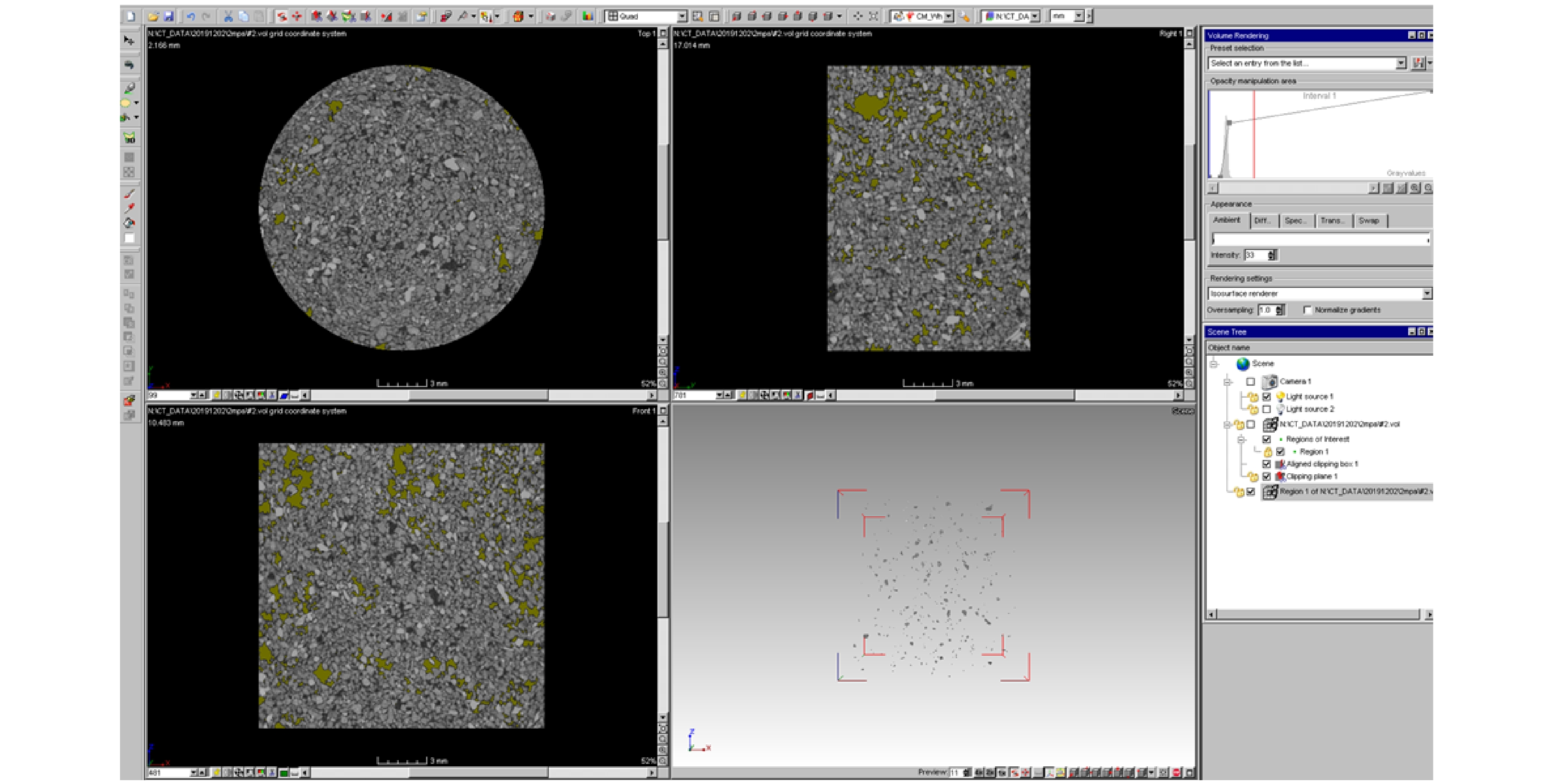
In this experiment, CT scanning was performed on the gas-bearing sediments in the reactor with no gas injection (atmospheric pressure was close to unsaturated soil), and it was then pressurized to 2 MPa, 4 MPa, and 6 MPa respectively. After each CT scan of sediment samples, 1 000 original CT images in three views (X-Y plane, X-Z plane and Y-Z plane of sediment) were obtained, which were preprocessed and exported by VG Studio MAX 2.1 software. The interface of software operation is shown in Fig. 2.

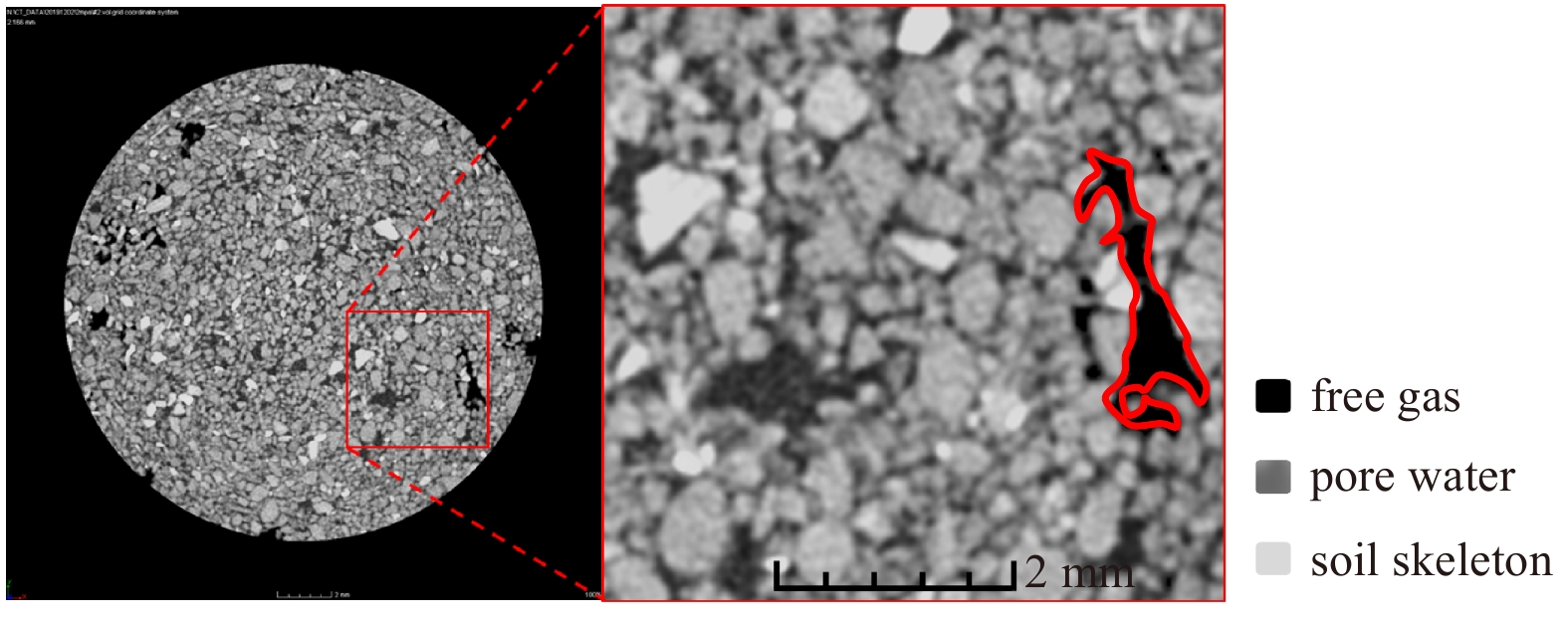
The gas-bearing soil sample at 2.166 mm was selected as the example, and its scanning image obtained by gas injection pressurization at 2 MPa gas reservoir pressure is analyzed. It can be seen from Fig. 3 that the part with the weakest X-ray absorption and the darkest color (black) is the bubble; the part with the strongest X-ray absorption and the lightest color is the soil skeleton. Some particles have a high density or a white color, which should be high-density solid particles such as quartz located between bubbles and solid particles. The grey color in the soil matrix is pore water, which fills in the pores of particles, and part of pore water even directly occupies the cavity of the soil skeleton.

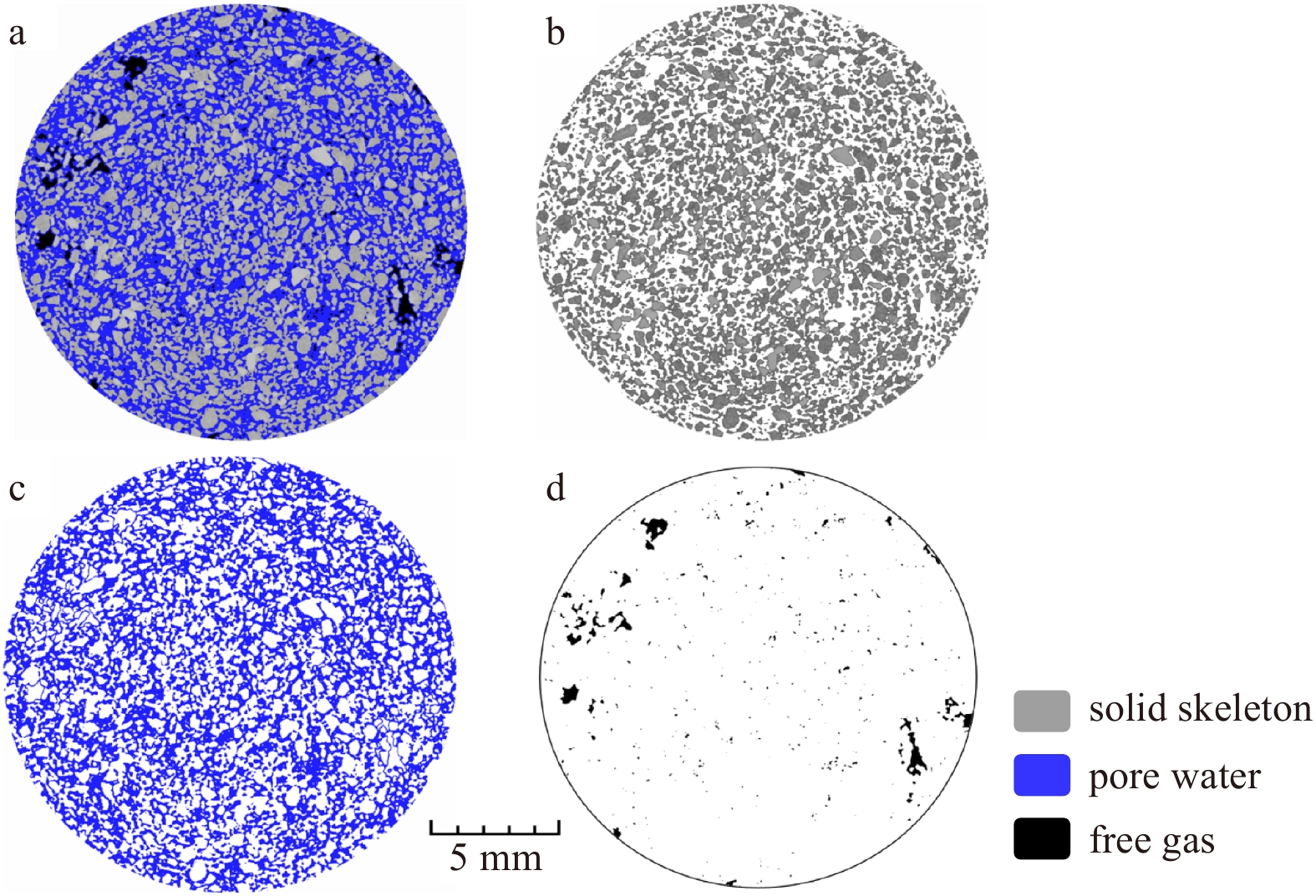
The visualization software Avizo was adopted to dye the CT image. Figure 4 shows the CT image of X-Y plane slice with the process of solid, liquid, and gas three-phase segmentation and coloring, where light gray is soil skeleton particles, blue is pore water, and black is a bubble. Figure 4b is the particle separation map of the solid medium, and the original gray image of CT is retained as well. It can be found that the density of sediment particles is also varied. Some particles with higher density show lighter color and larger volume than surrounding particles in the sediment, which may be quartz mineral particles. Figure 4c is the extracted liquid phase separation diagram, and the connectivity in the liquid phase is sound. The phenomenon of the pore water group is occupying the cavity. At the same time, large bubbles are surrounded by the pore water, and they even form a closed loop in the image. Figure 4d is the extracted gas-phase separation diagram. There are many large bubbles, and small bubbles are scattered in the middle.

To achieve a more vivid and intuitive comparison of the microscopic characteristics under different gas reservoir pressures, the intercepted CT image of the cube in the middle 2.17 mm is reconstructed, as shown in Fig. 5. It is evident that the shape of the bubble in the upper left corner of the cut-off sediment is rather stable under varied gas reservoir pressures. The bubble occupies all the pores, and the soil skeleton is relatively stable. Thus, the soil skeleton does not change with the gas reservoir pressure. When the pressure gas injection reaches 2 MPa, the number of small bubbles increases, while that of medium-sized decreases. When the pressure is increased to 6 MPa, the gas volume increases significantly, and the solid moves upward, as shown in Fig. 6. When the gas reservoir pressure in the reactor is reduced from 6 MPa to 3 MPa, the soil skeleton becomes more stable, and the pores and bubbles decrease in a more even manner. However, it should be noted that the shapes of bubbles with the increase of gas reservoir pressure are mostly irregular, except the bubbles at 0 MPa, which are slightly spherical. There may be a small channel existed to connect two main gas chambers. At the same time, when the gas reservoir pressure increases from 4 MPa to 6 MPa, the soil skeleton moves up.


Furthermore, the number and size of bubbles are analyzed, and the CT image with 4 MPa gas reservoir pressure is selected as an example. After the 3D reconstruction of the CT image, bubbles can be chosen in line with the bubbles’ gray value in Fig. 7 to facilitate identification. The total volume of sediment intercepted by CT is 4 039.25 mm3, in which the total volume of bubbles is 200.877 mm3, and the gas content is 4.97%. The number of bubbles and each volume is analyzed, and 10 184 bubbles are extracted accordingly. The equivalent half diameter range of bubbles is 0.013 5–2.513 mm, and the average bubble radius is 0.167 mm. The smallest bubble extracted from the image is a voxel point, which is a cube with a side length of 21.74 μm and an equivalent radius of 13.5 μm.

VG Studio MAX 2.1 was adopted to determine the threshold value. The gray value range of the solid, liquid, and gas phases of each CT scan slice is obtained accordingly. Image J is selected to acquire the proportion of voxel range corresponding to different substances in each CT image. For example, suppose the number of voxels in the gray value range of the gas phase and the number of voxels of a single slice in the scanned image are considered m and n. In that case, respectively, the percentage of m in n for the corresponding slice can be obtained, which is regarded as the apparent gas content. Taking the CT images of gas-bearing sediments without gas injection as an example, the two-dimensional segmentation and calculation of each CT image for a total of 803 X-Y planes were carried out, and the apparent gas content of each position within the z-axis height of 17.40 mm was obtained accordingly. The volume gas content of 4.97% showed the percentage of voxels, representing the sample’s gas state. The distribution curve of the apparent gas content along the soil sample was obtained with the sorted data, as shown in Fig. 8.

Similarly, the clear water cut and porosity distribution curve can be obtained as well, as shown in Fig. 9. The apparent water content fluctuates from 38% to 45%, and the apparent porosity vary from 44% to 49%, which reflects the spatial anisotropy of sediment particles. The calculated volumetric water content is 41.65%, which is slightly higher than 40% calculated in the preparation of the gas-bearing sediment samples. On the one hand, there is an inevitable fluctuation compared with the overall water content because CT image analysis is only accounting for a small part of the intercepted sediment samples. On the other hand, it may be that in the process of CT image segmentation, some light density solid particles show weak absorption to X-ray, and their gray level may be classified into pore water for approaching the segmentation threshold. It is also possible that the CT image analysis is accurate, but there are errors in the acquisition of geotechnical test parameters. Considering that the difference between the apparent water content obtained by CT image and the overall water content of the sample is only 1.65%, it is recognized here that both are reasonable values.

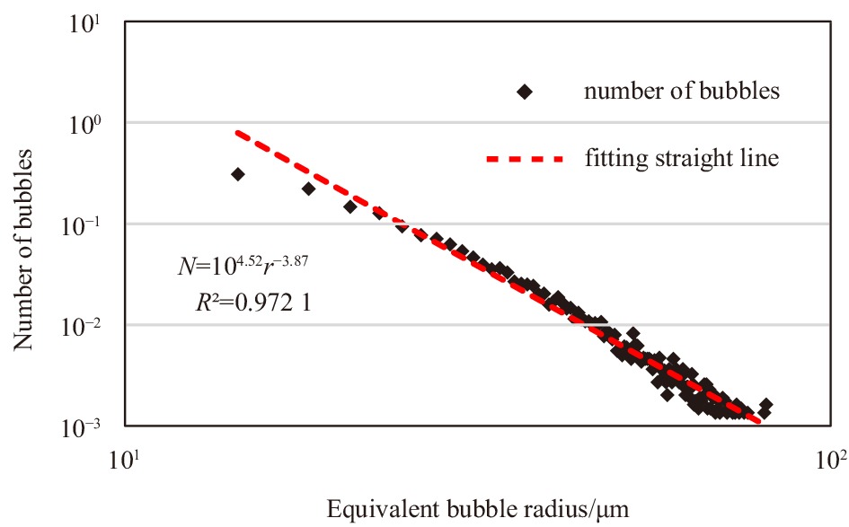
For the number of bubbles, it is more useful to consider the number of bubbles per unit volume. Taking the sample with gas reservoir pressure of 2 MPa as an example, the data of each bubble is extracted accordingly, and the relation between bubble number and radius in bubble size characteristics is analyzed in logarithmic coordinates, as shown in Fig. 10. At this time, the fitting Eq. (1) of bubble number and radius can be obtained as follows:

| $$ N{\text{ = }}{10^{4.52}}{r^{{\text{ − 3}}{\text{.87}}}} , $$ | (1) |
where N is the number of bubbles per unit volume in sediments; r is equivalent radius of bubble.
To observe and compare the micro-distribution characteristics of gas-bearing sediments under different gas reservoir pressure, the change of pressure can be further divided into pressure increasing stage and pressure releasing stage. Figure 11 shows the gas content obtained by CT scanning images of different positions in gas-bearing sediments at 0 MPa (i.e., the initial state of gas injection without pressure) and 2 MPa. The gas content at 2 MPa of each position in the deposit minus that at 0 MPa is obtained so that a more intuitive comparison can be gained.

It can be found that when pressure is increased to 2 MPa for methane gas, the volume gas content of some sediments intercepted will decrease from 4.97% to 4.63%. The gas content in different positions is varied, and the difference is rather large. For example, the gas content at 0–10 mm is relatively stable, and its value of change is within 1%, while the gas content at above 10 mm has a relatively significant decrease. The maximum range of reduction is close to 2%. If the volume gas content is considered as about 5%, it can be seen that the gas content is remarkably affected by the increase of gas injection pressure in the sediment sample.
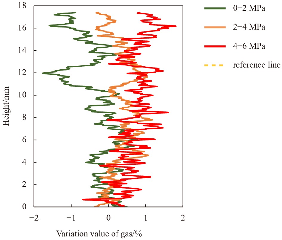
The changes in gas content with the increase of gas reservoir pressure are compared, as shown in Fig. 12. It can be seen that the volume of gas content starts to decrease when the pressure is increased to 2 MPa, while the gas content of sediment samples increases slightly. At the same time, the changing trend of the gas at the same position is not consistent, so the bubble does not always increase in one direction with the increase of gas reservoir pressure, but there is the role of flow and migration. As a result, the gas content in different positions may increase or decrease. It can be found that the apparent gas content of the gas-bearing sediment sample above 10 mm shows a more severe feature. In contrast, the initial gas content of this part is not significant compared with the situation at 2 MPa and 6 MPa with the location analysis. The gas contents at 2 MPa and 6 MPa are shown in Fig. 13, and the volume of gas content increases by near 1%. Overall, the sample with high gas content increases less. In contrast, the sample with low gas content increases more, which means that the distribution of volume gas content tends to be uniform with the position with the increase of gas reservoir pressure.


The microscopic characteristics of the gas reservoir in pressure releasing stage are analyzed. After the pressure is increased to 6 MPa, the pore water gas pressure is stabilized at a high-pressure value. With gas pressure released to 3 MPa, there is a pressure difference between the upper and lower positions of gas-bearing sediment samples driving liquid movement. The pressure difference makes the pore water move downward and fill the pores occupied by the original bubbles. Moreover, the content of the soil skeleton decreases with pore fluid. Therefore, to change the sediment reservoir with controlled outgassing, it is necessary to note the pore pressure changes when releasing the shallow gas on the seafloor. The reason is that the connected pore water can easily migrate in the reservoir, and its bulk modulus is much higher than that of the pore bubble, which may play a leading role in the microscopic changes of gas-bearing sediments.
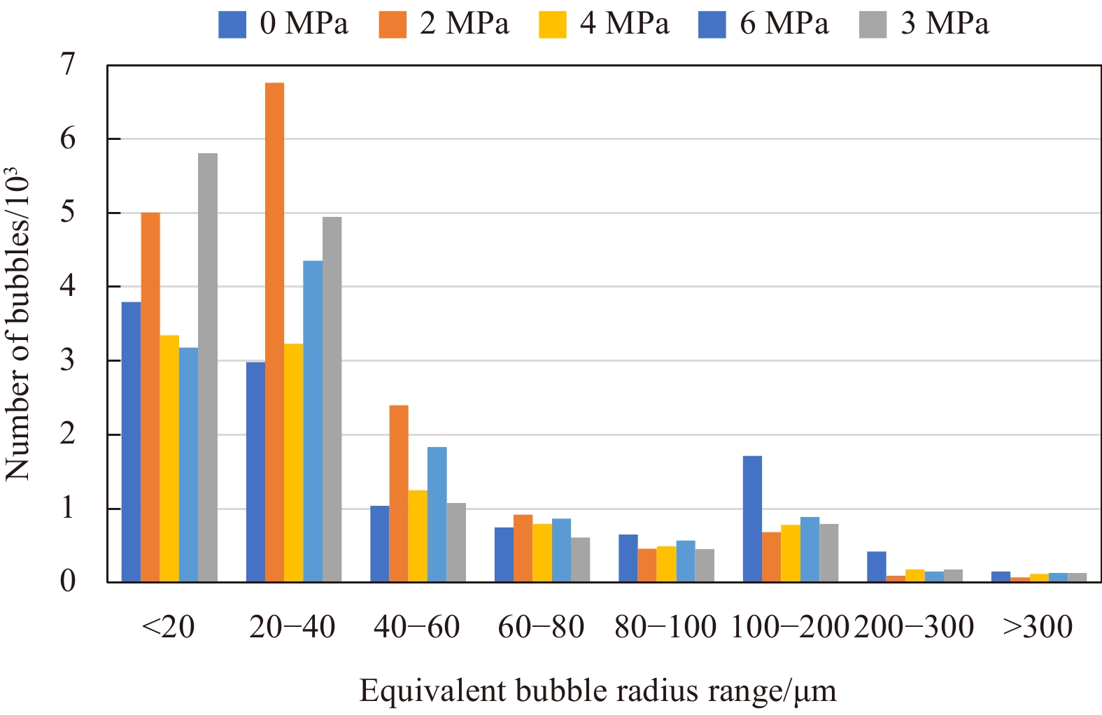
To compare the overall change of bubbles in gas-bearing sediments under the gas reservoir pressure, the number of bubbles in varied equivalent radius ranges is extracted, as shown in Fig. 14.

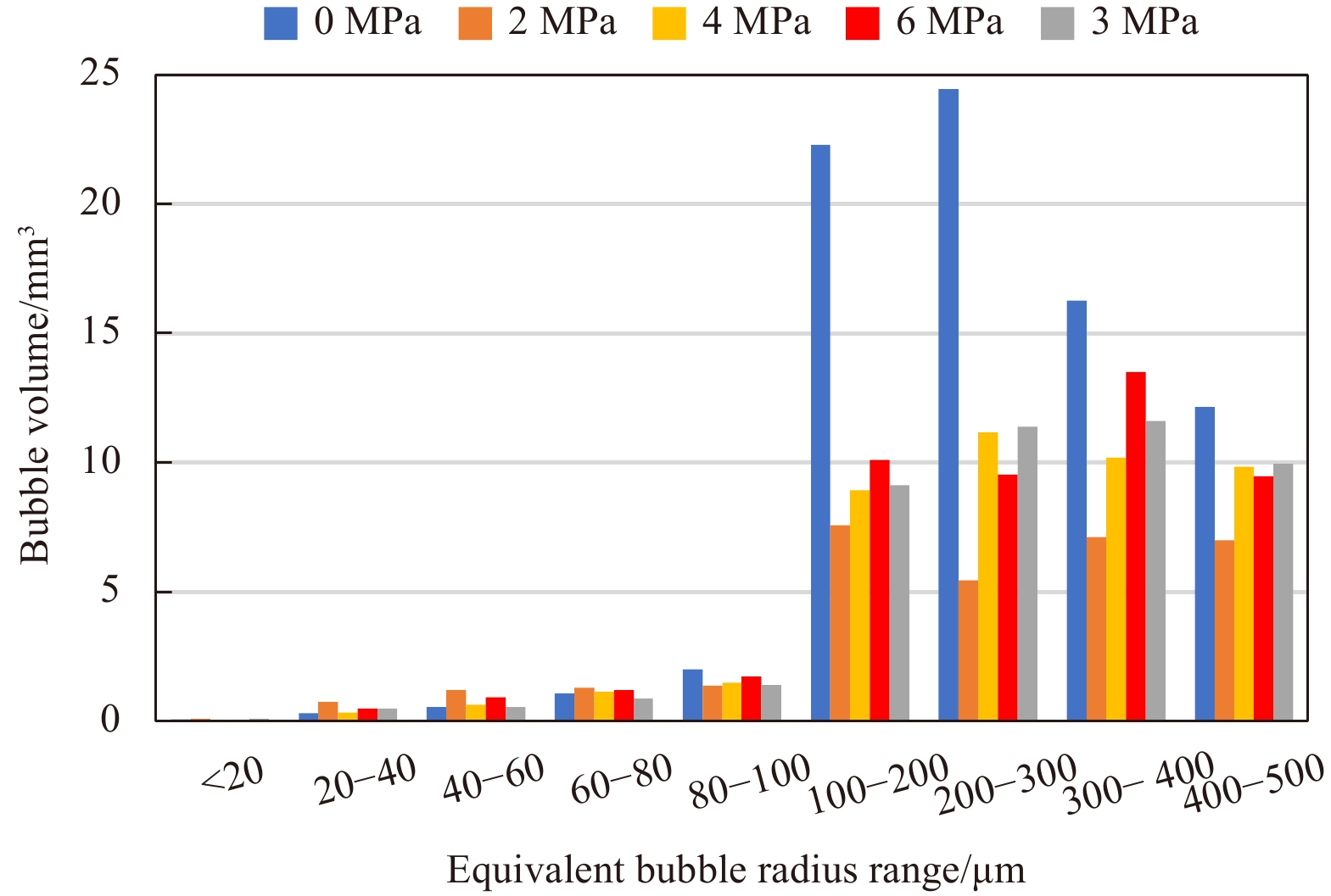
The numbers of bubbles with an equivalent radius of less than 40 μm are mainly small, and the difference is not recognizable anymore in the diagram after 0.3 mm. From the data, the number is the biggest when there is no gas reservoir pressure, and the smallest is at 2 MPa. Then with the increase of pressure, the number of bubbles increases. Due to the accuracy limit of CT, it is impossible to identify and extract smaller bubbles. The bubble volume for each equivalent radius range under different gas reservoir pressures is derived, as shown in Table 2. The gas contents of different equivalent radius are compared and analyzed, as shown in Fig. 15. It can be found that the bubble volume is lower when the equivalent radius is ranged less than 200 μm, accounting for less than 3%. The most significant difference appears in the gas volume with the equivalent radius greater than 500 μm. When the pressure of the sediment gas reservoir increases from 0 MPa to 2 MPa, the volume of bubbles whose equivalent radius is less than 80 μm increases, but the volume of bubbles larger than 80 μm decreases. With the equivalent radius of 80 μm as the borderline, when the pressure of the sediment gas reservoir increases from 2 MPa to 4 MPa, the bubble volume of small bubbles decreases, and that of large bubbles increases, which is in line with the change of bubble number. When the pressure of the sediment gas reservoir increases from 4 MPa to 6 MPa, the change of bubble volume becomes even more complicated. The bubble volume within 200 μm to 300 μm decreases and the bubble volume in other ranges changes little or increases. The trend of bubble volume in the pressure releasing stage is opposite to that of 4 MPa and 6 MPa, and the bubble volume within 200 μm to 300 μm increases, while the bubble volume in other ranges changes little or decreases, which may indicate that the bubble with an equivalent radius in the range of 200–300 μm is relatively closed. When the gas reservoir pressure increases from 4 MPa to 6 MPa, the bubble will be compressed. When the gas reservoir pressure is released from 6 MPa to 3 MPa, the bubble radius may increase slightly.
| Radius range/μm | Reservoir pressures/MPa | ||||
| 0 | 2 | 4 | 6 | 3 | |
| <20 | 0.064 | 0.090 | 0.057 | 0.058 | 0.100 |
| 20–40 | 0.304 | 0.753 | 0.338 | 0.497 | 0.491 |
| 40–60 | 0.545 | 1.196 | 0.650 | 0.931 | 0.549 |
| 60–80 | 1.067 | 1.288 | 1.131 | 1.211 | 0.888 |
| 80–100 | 2.000 | 1.384 | 1.491 | 1.718 | 1.392 |
| 100–200 | 22.302 | 7.574 | 8.933 | 10.096 | 9.137 |
| 200–300 | 24.447 | 5.450 | 11.176 | 9.535 | 11.389 |
| 300–400 | 16.269 | 7.115 | 10.188 | 13.503 | 11.609 |
| 400–500 | 12.142 | 6.988 | 9.849 | 9.482 | 9.945 |
| >500 | 120.636 | 160.066 | 157.064 | 188.412 | 174.696 |
| Summary | 199.776 | 191.905 | 200.877 | 235.442 | 220.196 |
DownLoad:
CSV

The microstructure of gas-bearing sediments was changed with pressurized gas injection, and the two-dimensional images obtained by CT testing were reconstructed with image processing software Avizo and image J. The internal pores of samples in different scanning stages are extracted as well. The microscopic characteristics of gas-bearing sediments characterized by CT images can be analyzed as follows.
(1) The analysis of two-dimensional and three-dimensional CT images of gas-bearing sediments can intuitively obtain the micro-distribution of the internal space with no influence on the sediments. Changing the gas reservoir pressure can be adopted to vividly compare the changes of a specific component in the sediments, which shows a better application effect of CT technology on the study of micro sediment characteristics.
(2) The volume and microscopic information of gas content change can be obtained by analyzing the gas content proportion in CT images at different positions of the sample. Even if the gas content in the reservoir deviates slightly, its changes can be measured more accurately than that of the liquid content.
(3) The number of bubbles decreases with the increase in radius. Under different gas reservoir pressures, the relations may change to some extent, and the effect of pressure release is particularly significant. The results show that the bubble volume of the sediment is different from that of other gas reservoirs with no pressure, indicating that the pressure released after sampling and measurement has a significant impact on the microscopic characteristics.
(4) The number and volume of bubbles in diverse equivalent radius ranges will change regularly under different gas reservoir pressure. Overall, with the increase of gas reservoir pressure, the number and volume of small bubbles decrease, while large bubbles increase. Based on the proposed reconstruction model of gas bearing soil under different gas reservoir pressures, it can be used to analyze the practical engineering problems in coastal shallow gas bearing strata, and provide experimental support for the safety research of gas bearing soil in marine engineering construction.
| [1] |
Anderson A L, Abegg F, Hawkins J A, et al. 1998. Bubble populations and acoustic interaction with the gassy floor of Eckernförde Bay. Continental Shelf Research, 18(14−15): 1807–1838. doi: 10.1016/S0278-4343(98)00059-4
|
| [2] |
Best A I, Tuffin M D J, Dix J K, et al. 2004. Tidal height and frequency dependence of acoustic velocity and attenuation in shallow gassy marine sediments. Journal of Geophysical Research: Solid Earth, 109(B8): B08101
|
| [3] |
Blunt M J, Bijeljic B, Dong H, et al. 2013. Pore-scale imaging and modelling. Advances in Water Resources, 51: 197–216. doi: 10.1016/j.advwatres.2012.03.003
|
| [4] |
Davis A M. 1992. Shallow gas: an overview. Continental Shelf Research, 12(10): 1077–1079. doi: 10.1016/0278-4343(92)90069-V
|
| [5] |
Esrig M I, Kirby R C. 1977. Implications of gas content for predicting the stability of submarine slopes. Marine Geotechnology, 2(1−4): 81–100. doi: 10.1080/10641197709379771
|
| [6] |
Fleischer P, Orsi T, Richardson M, et al. 2001. Distribution of free gas in marine sediments: a global overview. Geo-Marine Letters, 21(2): 103–122. doi: 10.1007/s003670100072
|
| [7] |
Hong Yi, Wang Lizhong, Ng C W W, et al. 2017. Effect of initial pore pressure on undrained shear behaviour of fine-grained gassy soil. Canadian Geotechnical Journal, 54(11): 1592–1600. doi: 10.1139/cgj-2017-0015
|
| [8] |
Jin S, Nagao J, Takeya S, et al. 2006. Structural investigation of methane hydrate sediments by microfocus X-ray computed tomography technique under high-pressure conditions. Japanese Journal of Applied Physics (in Japanese), 45(24−28): L714
|
| [9] |
Judd A, Hovland M. 2009. Seabed Fluid Flow: The Impact on Geology, Biology and the Marine Environment. Cambridge, UK: Cambridge University Press, 15–26
|
| [10] |
Kim G Y, Narantsetseg B, Kim J W, et al. 2014. Physical properties and micro-and macro-structures of gassy sediments in the inner shelf of SE Korea. Quaternary International, 344: 170–180. doi: 10.1016/j.quaint.2014.01.049
|
| [11] |
Li Ping, Du Jun, Liu Lejun, et al. 2010. Distribution characteristics of the shallow gas in Chinese offshore seabed. The Chinese Journal of Geological Hazard and Control (in Chinese), 21(1): 69–74
|
| [12] |
Riboulot V, Cattaneo A, Sultan N, et al. 2013. Sea-level change and free gas occurrence influencing a submarine landslide and pockmark formation and distribution in deepwater Nigeria. Earth and Planetary Science Letters, 375: 78–91. doi: 10.1016/j.jpgl.2013.05.013
|
| [13] |
Robb G B N, Leighton T G, Dix J K, et al. 2006. Measuring bubble populations in gassy marine sediments: a review. In: Proceedings of the Institute of Acoustics Spring Conference. Milton Keynes, UK: Institute of Acoustics, 60–68
|
| [14] |
Robb G B N, Leighton T G, Humphrey V F, et al. 2007. Investigating Acoustic Propagation in Gassy Marine Sediments using a Bubbly Gel Mimic. Southampton, UK: University of Southampton
|
| [15] |
Sobkowicz J C, Morgenstern N R. 1984. The undrained equilibrium behaviour of gassy sediments. Canadian Geotechnical Journal, 21(3): 439–448. doi: 10.1139/t84-048
|
| [16] |
Sultan N, Cochonat P, Canals M, et al. 2004. Triggering mechanisms of slope instability processes and sediment failures on continental margins: a geotechnical approach. Marine Geology, 213(1−4): 291–321. doi: 10.1016/j.margeo.2004.10.011
|
| [17] |
Sultan N, Garziglia S. 2014. Mechanical behaviour of gas-charged fine sediments: model formulation and calibration. Géotechnique, 64(11): 851–864
|
| [18] |
Thomas S D. 1987. The consolidation behaviour of gassy soil [dissertation]. Oxford, UK: University of Oxford, 61–69
|
| [19] |
Thomas S, Hill A J, Clare M, et al. 2011. Understanding engineering challenges posed by natural hydrocarbon infiltration and the development of authigenic carbonate. In: James J, Stephan U, eds. Proceedings of Offshore Technology Conference. Houston, TX, USA: Southampton Press, 164–167
|
| [20] |
Tuffin M D J. 2001. The geoacoustic properties of shallow, gas-bearing sediments [dissertation]. Southampton: University of Southampton, 44–67
|
| [21] |
Warner G S, Nieber J L, Moore I D, et al. 1989. Characterizing macropores in soil by computed tomography. Soil Science Society of America Journal, 53(3): 653–662. doi: 10.2136/sssaj1989.03615995005300030001x
|


Figures(15) / Tables(2)

Supported by:
Beijing Renhe Information Technology Co. Ltd


| Feature parameter | Value |
| Water content (ω) | 40.0% |
| Density (ρ) | 2.82 g/cm3 |
| Dry density (ρd) | 1.95 g/cm3 |
| Gravity specific (Gs) | 2.7 |
| Void ratio (e) | 0.71 |
| Porosity (n) | 43% |
DownLoad:
CSV
| Radius range/μm | Reservoir pressures/MPa | ||||
| 0 | 2 | 4 | 6 | 3 | |
| <20 | 0.064 | 0.090 | 0.057 | 0.058 | 0.100 |
| 20–40 | 0.304 | 0.753 | 0.338 | 0.497 | 0.491 |
| 40–60 | 0.545 | 1.196 | 0.650 | 0.931 | 0.549 |
| 60–80 | 1.067 | 1.288 | 1.131 | 1.211 | 0.888 |
| 80–100 | 2.000 | 1.384 | 1.491 | 1.718 | 1.392 |
| 100–200 | 22.302 | 7.574 | 8.933 | 10.096 | 9.137 |
| 200–300 | 24.447 | 5.450 | 11.176 | 9.535 | 11.389 |
| 300–400 | 16.269 | 7.115 | 10.188 | 13.503 | 11.609 |
| 400–500 | 12.142 | 6.988 | 9.849 | 9.482 | 9.945 |
| >500 | 120.636 | 160.066 | 157.064 | 188.412 | 174.696 |
| Summary | 199.776 | 191.905 | 200.877 | 235.442 | 220.196 |
DownLoad:
CSV
| Feature parameter | Value |
| Water content (ω) | 40.0% |
| Density (ρ) | 2.82 g/cm3 |
| Dry density (ρd) | 1.95 g/cm3 |
| Gravity specific (Gs) | 2.7 |
| Void ratio (e) | 0.71 |
| Porosity (n) | 43% |
| Radius range/μm | Reservoir pressures/MPa | ||||
| 0 | 2 | 4 | 6 | 3 | |
| <20 | 0.064 | 0.090 | 0.057 | 0.058 | 0.100 |
| 20–40 | 0.304 | 0.753 | 0.338 | 0.497 | 0.491 |
| 40–60 | 0.545 | 1.196 | 0.650 | 0.931 | 0.549 |
| 60–80 | 1.067 | 1.288 | 1.131 | 1.211 | 0.888 |
| 80–100 | 2.000 | 1.384 | 1.491 | 1.718 | 1.392 |
| 100–200 | 22.302 | 7.574 | 8.933 | 10.096 | 9.137 |
| 200–300 | 24.447 | 5.450 | 11.176 | 9.535 | 11.389 |
| 300–400 | 16.269 | 7.115 | 10.188 | 13.503 | 11.609 |
| 400–500 | 12.142 | 6.988 | 9.849 | 9.482 | 9.945 |
| >500 | 120.636 | 160.066 | 157.064 | 188.412 | 174.696 |
| Summary | 199.776 | 191.905 | 200.877 | 235.442 | 220.196 |
 DownLoad:


 DownLoad: