Figure
1.
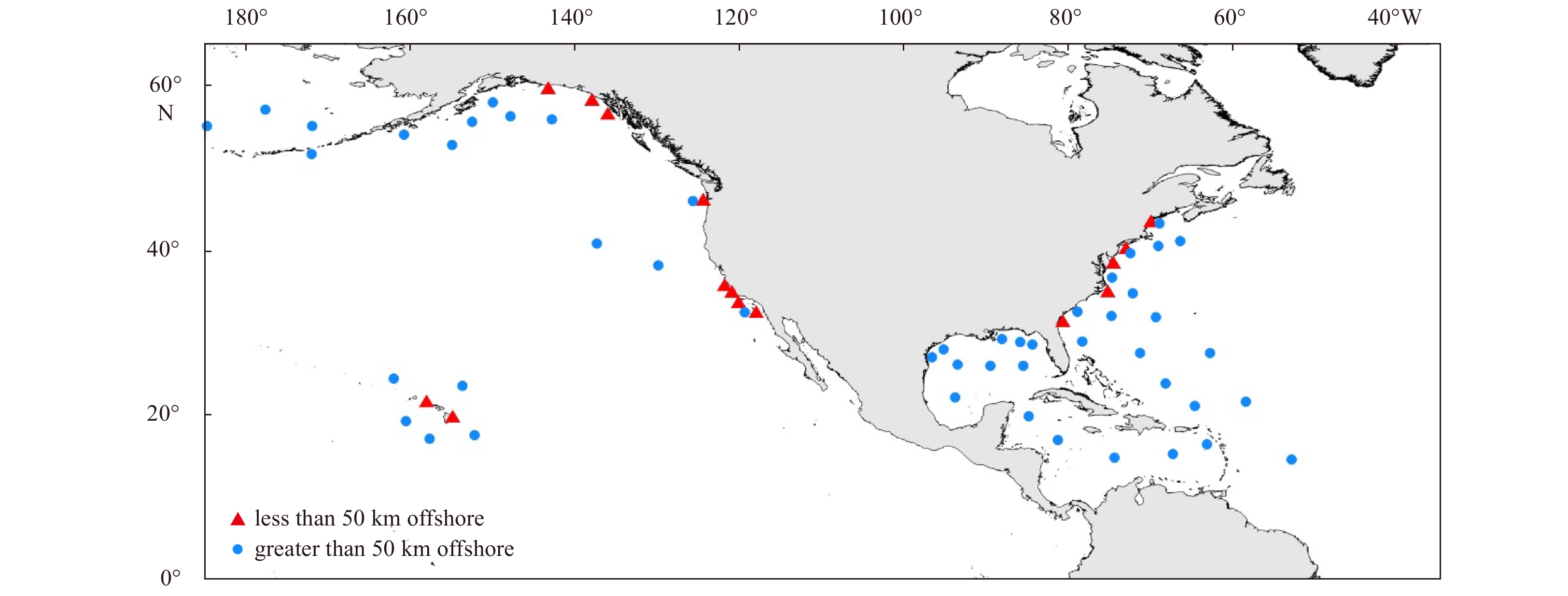
Location of 64 NDBC buoys selected.
| Citation: | Jing Ye, Yong Wan, Yongshou Dai. Quality evaluation and calibration of the SWIM significant wave height product with buoy data[J]. Acta Oceanologica Sinica, 2021, 40(10): 187-196. doi: 10.1007/s13131-021-1835-x

|
Waves are a vital movement process of the ocean surface, and wave observations are of great significance in studying marine environmental characteristics. The significant wave height (SWH) is one of the main parameters that describe wave characteristics. Long time series and stable continuous SWH data are necessary to evaluate global wave height changes (Chelton et al., 1981; Young et al., 2011). SWH data are widely used in waves and other ocean process model validation, wave climate surveys, ocean dynamics monitoring, disaster prediction, and many other research fields (Durrant et al., 2009).
In general, there are three methods of obtaining wave data: field observation, numerical simulation, and satellite remote sensing. Traditional field observations are usually achieved by measuring ships, tide stations, or buoys. The observation position of this method is concentrated in the nearshore area, so the data coverage is limited. However, due to high reliability, field observations are often used to verify the accuracy of wave data obtained by other methods (Collard et al., 2005; Wan et al., 2015). Numerical simulation is used to obtain high-resolution historical wave data and forecast data through computer simulations. However, due to the large amount of information processed in this way, the requirements for computer performance and algorithms are very high. At present, simulations are often used in the field of data reanalysis and numerical forecasting. With the development of satellite and sensor technologies, radar altimeters, synthetic aperture radar (SAR), and surface wave investigation and monitoring (SWIM) have also been used in wave observations. Satellite remote sensing continuously obtains ocean observation data on a global scale, which has a significant advantage over field observations. However, due to the influence of land echoes in the nearshore sea area, the wave detection accuracy of radar is not as good as that in the open sea (Brooks et al., 1990). In addition, differences also exist in the wave accuracies of different sea states (Yang and Zhang, 2019). Therefore, it is necessary to evaluate the applicability of radar data under different offshore distances and sea states.
High-precision SWH data play an essential role in wave research, so it is of great significance to carry out data evaluation and calibration, which can provide references for the application of SWH data and improve the data accuracy. There have been many relevant studies in recent years. Durrant et al. (2009) evaluated the SWH quality of Jason-1 and Envisat altimeters using buoys of the National Data Buoy Center (NDBC) and the Marine Environmental Data Service (MEDS) and improved the root mean squared error (RMSE) of Envisat from 0.219 m to 0.203 m by linear calibration. Jiang et al. (2018), Wang et al. (2018), and Liu et al. (2016b) verified that the precision of HY-2A SWH met the basic needs of practical application through buoy data and cross-comparison. Chen et al. (2017) evaluated the HY-2 Ku band SWH with buoy and Jason-2 data, and the results showed that the linear regression method could improve the data quality. Liu et al. (2016a) calibrated and verified the 1−9 m SWH of HY-2 with the dual-branch method using buoy and multiple altimeter data. Peng and Lin (2016) and Xu et al. (2016) proposed the calibration of HY-2A SWH by using the total least square method and GNSS buoy method, and the accuracies of both methods were improved. Yang and Zhang (2019) compared Sentinel-3A/3B SWH with buoys and concluded that the data were of high accuracy that declines with increasing SWH.
From the above studies, it can be seen that researchers have carried out much work on data quality evaluation and calibration of SWH. With regard to SWH data quality evaluation, to analyze the wave observation applicable situation of each instrument, these studies used many statistical parameters and classified data from a variety of perspectives and provided reliable references for users of these SWH products. With regard to SWH data calibration, different calibration models and methods were selected, and the data accuracies after calibration were significantly improved. The calibration effects of nonlinear methods were generally better than those of linear methods. It can be predicted that using nonlinear methods is the trend of data calibration.
SWIM is a new type of wave information detection instrument based on real aperture radar (RAR). It provides data on a globally large and long time series normalized radar cross section (NRCS), wave direction spectrum, wind speed, and wave height information. Based on the current research status of SWH quality evaluation and calibration, most of studies focus on altimeters. Due to the long running time of many radar altimeters, they provide long periods of global sea surface observation data. Because of differences between SWIM and altimeters in instrument parameters and operating modes, the ability of SWIM to detect waves is anticipated and of interest. However, very few studies have been conducted to evaluate the quality of SWIM data. Therefore, to understand the quality of SWIM SWH products, analyzing differences in wave detection capabilities under different conditions and exploring ways to improve data accuracy are necessary.
In this paper, quality evaluation and calibration of SWIM SWH were carried out. The SWH data of SWIM and NDBC buoys were collected and time-space matched. The accuracies of SWIM SWH were calculated and analyzed under different offshore distances and sea states. Moreover, according to the results of the traditional calibration method, the limitations were analyzed and an improved calibration method based on sea state segmentation was proposed. The effectiveness and superiority of this method were verified. The influence of spatiotemporal window selection on data quality evaluation was also analyzed.
SWIM is a wave scatterometer developed by the Centre National d’Etudes Spatiales (CNES). It was launched in October 2018 as one of the payloads of the China France Oceanography SATellite (CFOSAT). The instrument is used to detect waves on the ocean surface, study wave characteristics and distribution, and improve the abilities of marine meteorological prediction and climate change perception. SWIM is the first spaceborne sensor to obtain the wave direction spectrum and sea surface wind speed with multiple azimuthal directions and incidence angles. It has an orbital altitude of 519 km and operates simultaneously in beams with six incident angles (0°, 2°, 4°, 6°, 8°, and 10°), allowing 360° azimuth rotation scanning with an antenna rotation speed of 5.6 r/min. Similar to the altimeter, the nadir beam of SWIM detects sea surface SWH and wind speed; 6°, 8°, and 10° beams are used to estimate the wave direction spectrum and wave parameters; and the backscattering coefficient can be measured at all beam angles (Grelier et al., 2016; Hauser et al., 2017; Suauet et al., 2018). In this paper, the SWIM Level 2 data product was obtained from August 2019 to June 2020 through the AVISO data center, and the SWH data used were provided in the unit of the box (size of the box: 70 km×90 km).
Buoy data are often used as a reference value for accuracy verification and quality evaluation of radar data. In this paper, data from the NDBC buoys of the National Oceanic and Atmospheric Administration (NOAA) were used for SWIM SWH validation. The specific locations of the 64 buoys selected are shown in Fig. 1, and Table 1 lists their basic information. There are 15 buoys at an offshore distance of less than 50 km and 49 buoys at greater than 50 km.
| Buoy ID | Latitude | Longitude | Offshore distance/km | Serial number |
| 51206 | 19.780°N | 154.970°W | 5.45 | A1 |
| 51201 | 21.671°N | 158.117°W | 5.50 | A2 |
| 44007 | 43.525°N | 70.141°W | 6.77 | A3 |
| 46069 | 33.677°N | 120.213°W | 23.65 | A4 |
| 41025 | 35.025°N | 75.363°W | 25.86 | A5 |
| 46011 | 34.956°N | 121.019°W | 29.92 | A6 |
| 41008 | 31.400°N | 80.866°W | 33.59 | A7 |
| 44009 | 38.457°N | 74.702°W | 34.43 | A8 |
| 46082 | 59.681°N | 143.372°W | 37.40 | A9 |
| 44025 | 40.251°N | 73.164°W | 38.13 | A10 |
| 46028 | 35.774°N | 121.905°W | 41.37 | A11 |
| 46029 | 46.143°N | 124.485°W | 41.67 | A12 |
| 46086 | 32.499°N | 118.052°W | 43.68 | A13 |
| 46084 | 56.622°N | 136.102°W | 44.78 | A14 |
| 46083 | 58.268°N | 138.019°W | 48.96 | A15 |
| 41004 | 32.501°N | 79.099°W | 56.79 | B1 |
| 44005 | 43.201°N | 69.128°W | 63.16 | B2 |
| 42020 | 26.968°N | 96.693°W | 67.90 | B3 |
| 46072 | 51.672°N | 172.088°W | 68.13 | B4 |
| 42040 | 29.208°N | 88.226°W | 75.25 | B5 |
| 42060 | 16.433°N | 63.331°W | 79.16 | B6 |
| 46047 | 32.404°N | 119.506°W | 81.13 | B7 |
| 42019 | 27.910°N | 95.345°W | 88.26 | B8 |
| 44014 | 36.609°N | 74.842°W | 100.57 | B9 |
| 44008 | 40.504°N | 69.248°W | 103.99 | B10 |
| 46075 | 53.983°N | 160.817°W | 105.80 | B11 |
| 42039 | 28.788°N | 86.008°W | 109.11 | B12 |
| 44066 | 39.618°N | 72.644°W | 112.39 | B13 |
| 42036 | 28.501°N | 84.516°W | 119.57 | B14 |
| 51101 | 24.361°N | 162.075°W | 130.72 | B15 |
| 42057 | 16.908°N | 81.422°W | 141.80 | B16 |
| 46080 | 57.947°N | 150.042°W | 143.26 | B17 |
| 46078 | 55.556°N | 152.582°W | 158.91 | B18 |
| 41010 | 28.878°N | 78.485°W | 160.51 | B19 |
| 46089 | 45.925°N | 125.771°W | 171.78 | B20 |
| 42056 | 19.820°N | 84.945°W | 193.92 | B21 |
| 42055 | 22.124°N | 93.941°W | 199.32 | B22 |
| 41043 | 21.030°N | 64.790°W | 231.39 | B23 |
| 44011 | 41.070°N | 66.588°W | 239.24 | B24 |
| 51003 | 19.175°N | 160.625°W | 247.64 | B25 |
| 46073 | 55.009°N | 172.011°W | 256.98 | B26 |
| 42059 | 15.252°N | 67.483°W | 268.69 | B27 |
| 46070 | 55.008°N | 175.183°E | 270.43 | B28 |
| 51002 | 17.043°N | 157.742°W | 272.61 | B29 |
| 42003 | 25.925°N | 85.615°W | 298.36 | B30 |
| 42058 | 14.776°N | 74.548°W | 298.62 | B31 |
| 42001 | 25.942°N | 89.657°W | 298.74 | B32 |
| 41002 | 31.973°N | 74.958°W | 304.83 | B33 |
| 46066 | 52.765°N | 155.009°W | 305.47 | B34 |
| 51004 | 17.533°N | 152.255°W | 322.04 | B35 |
| 41001 | 34.724°N | 72.317°W | 324.03 | B36 |
| 42002 | 26.055°N | 93.646°W | 330.52 | B37 |
| 51000 | 23.528°N | 153.792°W | 351.38 | B38 |
| 46001 | 56.232°N | 147.949°W | 353.55 | B39 |
| 41046 | 23.822°N | 68.384°W | 358.85 | B40 |
| 46085 | 55.883°N | 142.882°W | 418.63 | B41 |
| 41047 | 27.514°N | 71.494°W | 449.00 | B42 |
| 41048 | 31.831°N | 69.573°W | 470.60 | B43 |
| 41044 | 21.582°N | 58.630°W | 500.93 | B44 |
| 46035 | 57.016°N | 177.703°W | 509.45 | B45 |
| 41049 | 27.490°N | 62.938°W | 511.85 | B46 |
| 46059 | 38.094°N | 129.951°W | 599.14 | B47 |
| 41040 | 14.554°N | 53.045°W | 652.81 | B48 |
| 46006 | 40.782°N | 137.397°W | 1284.26 | B49 |
| Note: The longitude and latitude range in the table are 0°–180°W, 0°–180°E, and 0°–90°N, and buoys are numbered according to offshore distance, with those shorter than 50 km numbered A and others numbered B. | ||||
 DownLoad:
CSV
DownLoad:
CSV
The outliers in the observed data affect the accuracy results, so the data must be preprocessed to eliminate outliers before evaluation and calibration. According to the flags of quality control, rainfall, and surface observation type in the satellite data products, the data with unqualified quality and under rain, land, and sea ice conditions were eliminated. Meanwhile, as the evaluation results of SWH under 0.5 m were greatly affected by errors, such data also need to be eliminated. For buoy SWH data, due to its fixed update frequency, the default value 99 during the period when data were not updated is invalid. Time-space matching parameters including time, longitude, latitude, and SWH were extracted from SWIM and buoys.
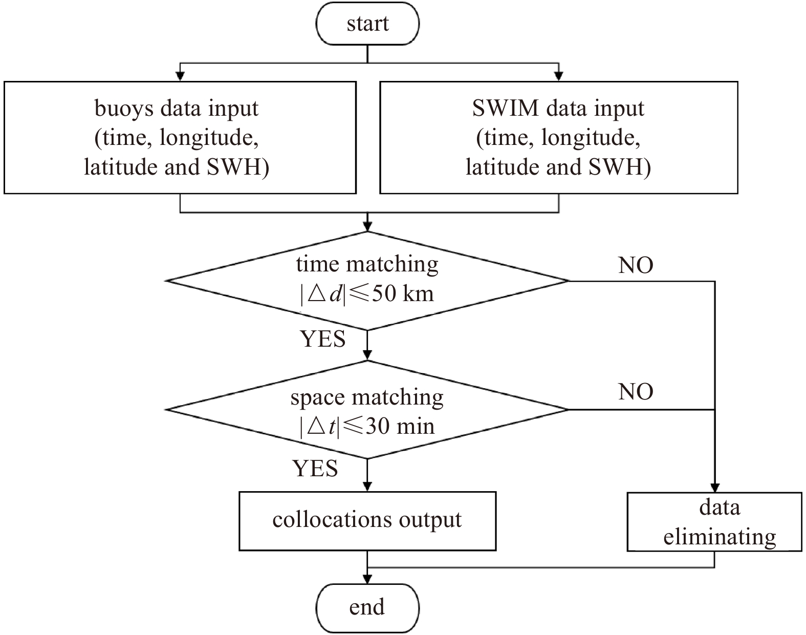
SWIM SWH quality evaluation verifies the data accuracy by comparing the synchronized SWIM and buoy data in time and space. Thus, the first step is data time-space matching to obtain point collocations. Considering the low probability of complete spatiotemporal coincidence between SWIM data and buoy data, it is necessary to set spatiotemporal windows to limit data differences. The point collocations that meet the window conditions are extracted and considered to be matching data corresponding to the same space-time point. Time-space matching hopes to obtain as many collocations and little spatiotemporal data difference as possible, so the selection of a spatiotemporal window is critical.
The temporal and spatial windows selected in this paper were 50 km and 30 min, indicating that the spatial gap between SWIM and buoy data was less than 50 km and that the time interval was less than 30 min (Gower, 1996; Queffeulou, 2003). The process of time-space matching between SWIM data and buoy data is shown in Fig. 2.

The statistical parameters used to validate the SWIM SWH product, including RMSE, relative error (RE), and scatter index (SI), are defined as follows:
| $$ {\text{RMSE}} = \sqrt {\frac{1}{n}\sum\limits_{i = 1}^n {{{\left( {{A_i} - {B_i}} \right)}^2}} } , $$ | (1) |
| $$ {\text{RE}} = \frac{1}{n}\sum\limits_{i = 1}^n {\left( {\frac{{\left| {{A_i} - {B_i}} \right|}}{{{B_i}}}} \right)} \times 100\text{%} , $$ | (2) |
| $$ {\text{SI}} = \frac{{\sqrt {\dfrac{1}{n}\displaystyle\sum\limits_{i = 1}^n {{{\left[ {\left( {{A_i} - \bar A} \right) - \left( {{B_i} - \bar B} \right)} \right]}^2}} } }}{{\bar B}} , $$ | (3) |
where
The radar ocean detection principle derives parameters from the received sea echoes. Due to the influence of land in the nearshore sea area, the radar data accuracy is lower than that of the area away from the coast (Brooks et al., 1990; Deng et al., 2002). To analyze the SWH detection capabilities of SWIM at different offshore distances, the matching data of buoys and SWIM were classified according to whether the offshore distance of the buoy was greater than 50 km (Yang et al., 2010), and the classified data qualities were evaluated.
Sea states refer to the surface features caused by wind waves and swells in marine hydrographic observations, and SWH values vary by sea state. The wave level is the degree of fluctuation caused by the strength of the wind. To verify the accuracies of SWIM SWH in different sea states, the wave level table developed by the State Oceanic Administration (SOA) was taken as the classification standard in this paper (State Oceanic Administration, 2008), and SWH qualities in various sea states were evaluated. Table 2 is the wave level table.
| Wave level | SWH range/m | Sea state |
| 0 | SWH=0 | calm-glassy |
| 1 | SWH<0.1 | calm-rippled |
| 2 | 0.1≤SWH<0.5 | smooth-wavelet |
| 3 | 0.5≤SWH<1.25 | slight |
| 4 | 1.25≤SWH<2.5 | moderate |
| 5 | 2.5≤SWH<4.0 | rough |
| 6 | 4.0≤SWH<6.0 | very rough |
| 7 | 6.0≤SWH<9.0 | high |
| 8 | 9.0≤SWH<14.0 | very high |
| 9 | 14.0≤SWH | phenomenal |
DownLoad:
CSV
The SWIM SWH data calibration in this paper was based on the nonlinear least-squares fitting method (Xu et al., 2014). This method took the buoy SWH value as the standard, the minimum value of the sum of the squared errors of SWIM and buoy SWH as the target, carried out nonlinear fitting to SWIM SWH to obtain calibration factors, and calculated the calibrated SWH through the following formula:
| $$ y = a{x^2} + bx + c, $$ | (4) |
where a, b, and c represent the nonlinear calibration factors, x is the raw value of SWIM SWH, and
The traditional calibration method takes all data as a whole, obtains a set of factors through the fitting process, and uses the calibration formula to obtain the calibrated results of the data. Since the traditional method did not take the uneven distribution of point collocation numbers in different sea states into account, an improved data calibration method was proposed in this paper. The improved method segmented SWIM SWH data using the wave level table as the sea state classification standard, calibrated the data in each segment separately, and combined all the calibrated segments as the overall calibration results. The distribution difference of point collocation numbers in various sea states was considered in the improved method.
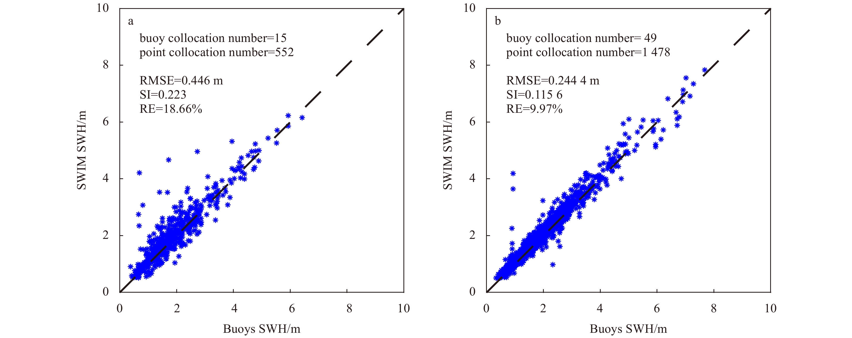
Based on the statistical parameters and offshore distance classification standard introduced in the methods section, the SWIM SWH accuracies at different offshore distances were calculated. The collocation scatterplot of SWIM and buoys is shown in Fig. 3. The numbers of buoy and point collocations with an offshore distance of less than 50 km are 15 and 552 with a 0.446 0-m RMSE, 18.66% RE, and 0.223 0 SI. When the offshore distance is greater than 50 km, the buoy and point collocation numbers are 49 and 1 478, with RMSE of 0.244 4 m, RE of 9.97%, and SI of 0.115 6.

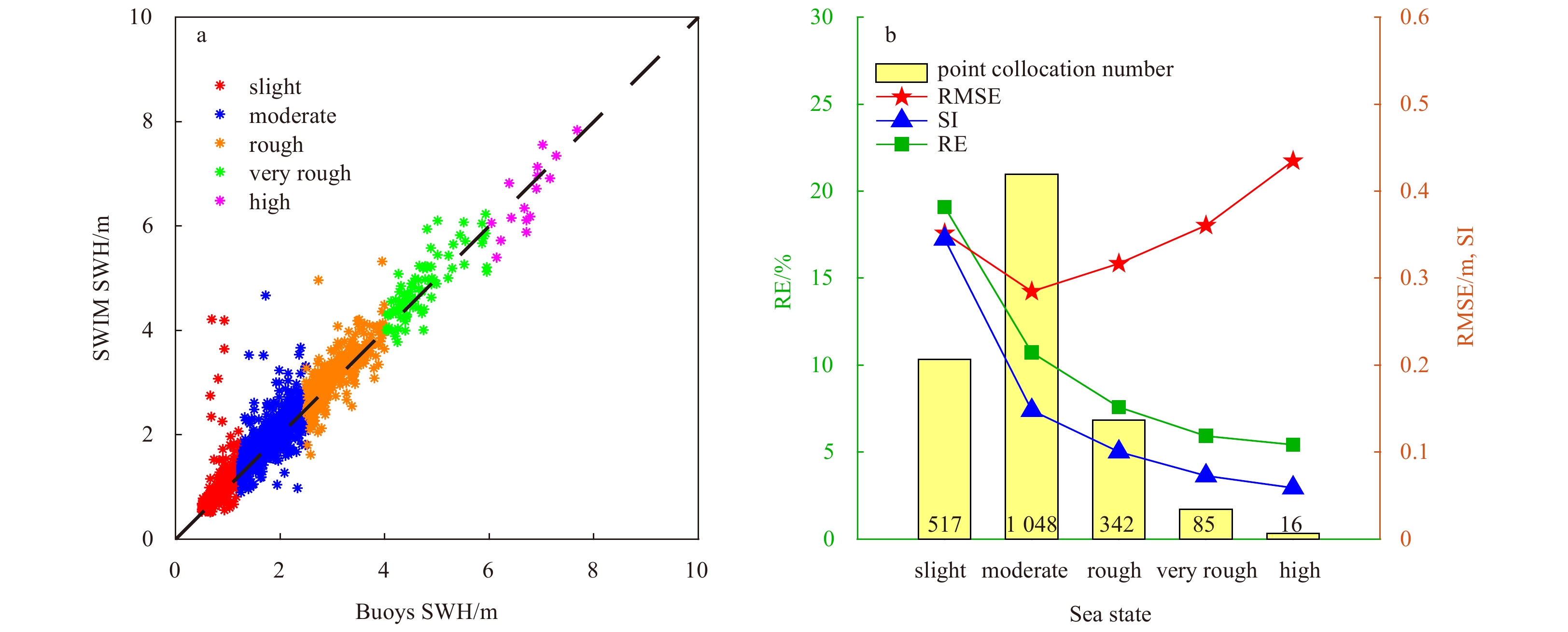
Similarly, based on the sea state classification standard, SWIM SWH data were classified into five types of sea states, and the accuracy in each sea state was calculated. The specific accuracy results are listed in Table 3, and Fig. 4 shows a scatterplot and comparisons of the validation results in different sea states. As indicated in the table and figure, with an increase in the SWH value in the corresponding sea states, the point collocation numbers are 517, 1 048, 342, 85, and 16. SI and RE both decrease with increasing SWH, while the maximum RMSE of 0.434 9 m is in the high sea state, and the minimum RMSE of 0.284 8 m is in the moderate sea state.
| Sea state | RMSE/m | SI | RE/% |
| Slight | 0.351 8 | 0.345 0 | 19.09 |
| Moderate | 0.284 8 | 0.148 1 | 10.73 |
| Rough | 0.316 9 | 0.100 4 | 7.59 |
| Very rough | 0.360 7 | 0.072 9 | 5.93 |
| High | 0.434 9 | 0.059 0 | 5.43 |
DownLoad:
CSV

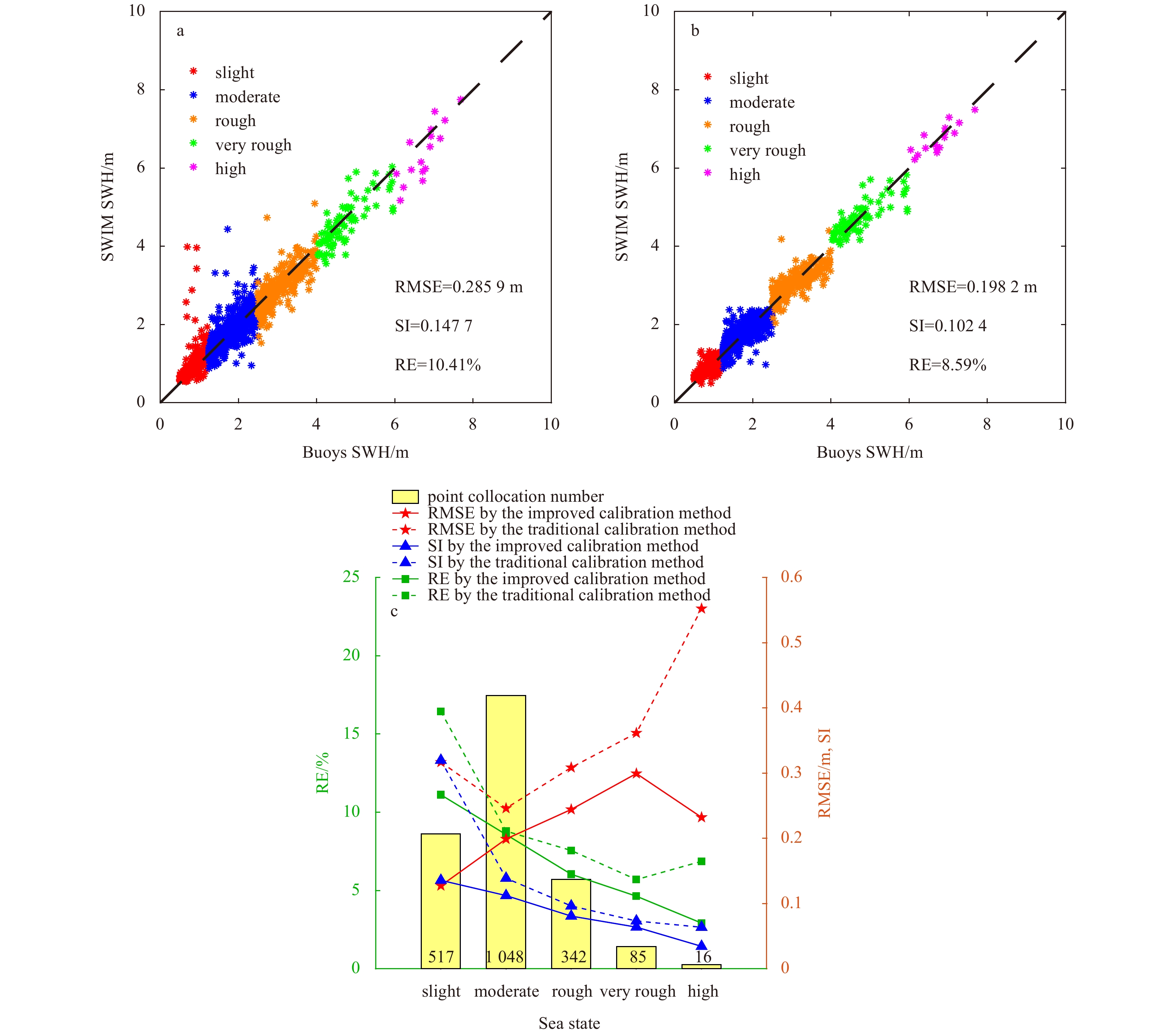
SWIM SWH data were calibrated by both the traditional and the improved methods. The nonlinear calibration factors of the two methods are listed in Tables 4 and 5. In the traditional method, to compare with the results of the improved method, the overall calibrated data were segmented according to the wave level table, and corresponding accuracies in different sea states were calculated using the same calibration coefficients. Figure 5a shows the scatterplot after calibration. The calibrated accuracy results are shown in Table 6, and the last row shows the overall calibrated accuracy. By the traditional calibration method, the overall RMSE decreased from 0.313 5 m to 0.285 9 m with an improved degree of 8.80%. However, the effects of the traditional method in various sea states are obviously different.
| a | b | c |
| 0.014 9 | 0.860 0 | 0.095 4 |
DownLoad:
CSV
| Sea state | a | b | c |
| Slight | −0.231 0 | 1.065 1 | 0.092 1 |
| Moderate | −0.231 0 | 1.591 5 | −0.363 4 |
| Rough | −0.011 4 | 0.717 0 | 0.905 0 |
| Very rough | 0.090 2 | −0.175 7 | 3.422 3 |
| High | 0.082 4 | −0.568 3 | 6.886 1 |
DownLoad:
CSV

| Sea state | Point collocation number | Raw RMSE/m | Traditional calibration RMSE/m (Degree of RMSE improvement) | Improved calibration RMSE/m (Degree of RMSE improvement) |
| Slight | 517 | 0.351 8 | 0.317 0 (+9.89%) | 0.127 5 (+63.76%) |
| Moderate | 1 048 | 0.284 8 | 0.246 2 (+13.55%) | 0.199 1 (+30.09%) |
| Rough | 342 | 0.316 9 | 0.308 7 (+2.59%) | 0.244 4 (+22.88%) |
| Very rough | 85 | 0.360 7 | 0.361 7 (−0.28%) | 0.299 5 (+16.97%) |
| High | 16 | 0.434 9 | 0.552 5 (−27.04%) | 0.232 3 (+46.59%) |
| All sea states | 2 008 | 0.313 5 | 0.285 9 (+8.80%) | 0.198 2 (+36.78%) |
DownLoad:
CSV
The scatterplot after calibration by the improved method and comparisons of calibration accuracy results using two methods are shown in Figs 5b and c. To compare the effects of the two calibration methods more specifically, the calibrated accuracies of the two methods along with the raw accuracies are listed in Table 6. The overall RMSE is reduced from 0.313 5 m of the raw data to 0.198 2 m of the improved calibration with an improved degree of 36.78%. The calibration results show that the improved method significantly improved the accuracy of SWH in all sea states.
In terms of the point collocation numbers between buoys and SWIM, Fig. 3 indicates that the collocation number at offshore distances greater than 50 km is relatively higher, which means that the data at that distance used for validation are more abundant. In regard to the SWH value distribution, the values at both offshore distances are densely distributed in the range below 4 m, while those above 4 m are lower. Considering the data accuracy, the RMSEs of both offshore distances are less than 0.5 m, and the RMSE at distances greater than 50 km is lower. The comparison result of REs is similar to that of the RMSEs. The SI results show that the data distribution at less than 50 km is more dispersed. Therefore, the quality of SWIM SWH at offshore distances greater than 50 km is better than that at distances less than 50 km.
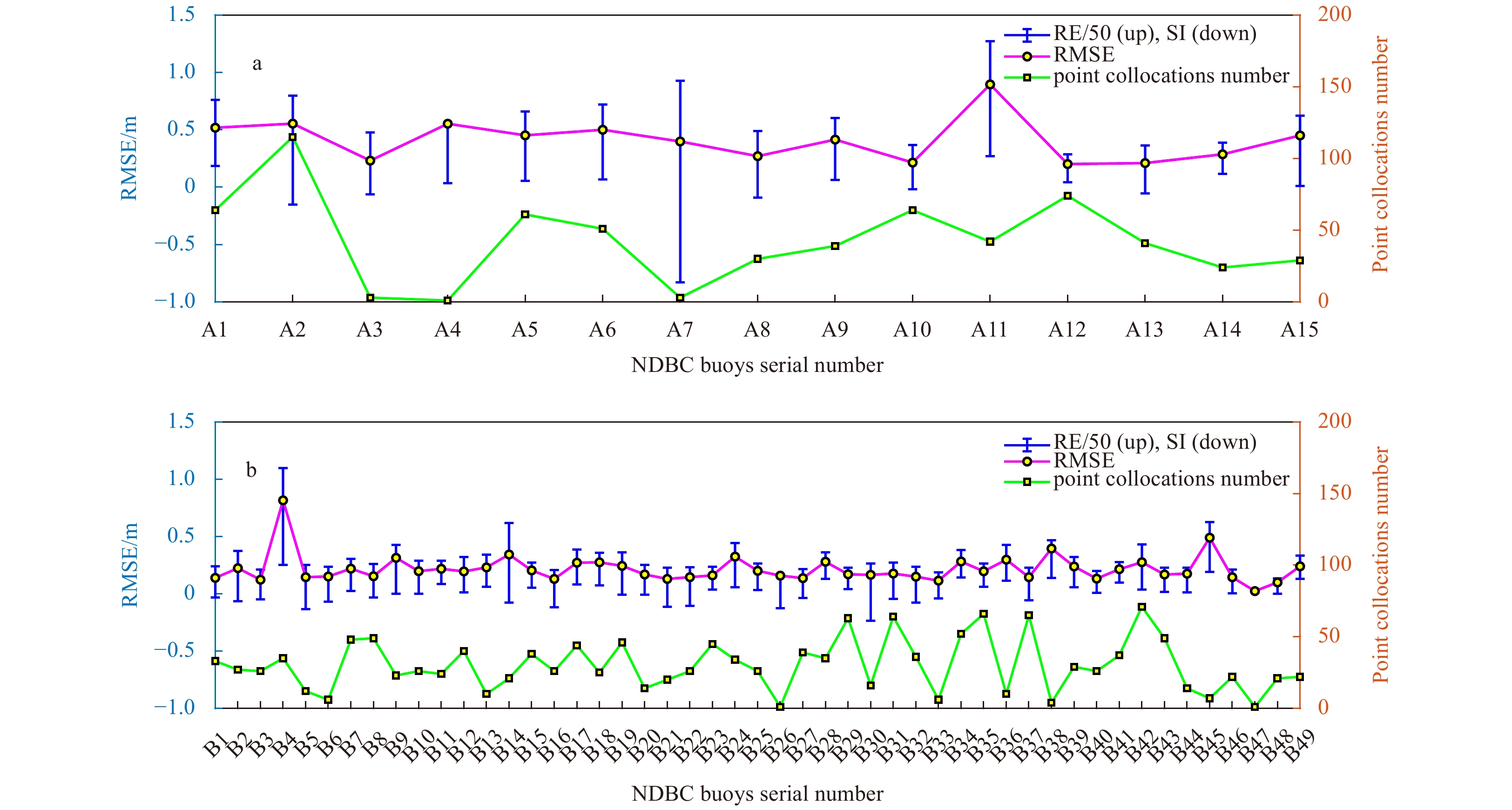
To explore the influence of offshore distance on the accuracy of SWH data in more detail, this paper also carried out product accuracy calculations based on buoy data classification. Figure 6 shows the collocation numbers and accuracy results for the SWIM SWH product with different buoy data. On average, the SWIM SWH product matches 37 points per buoy for A1–A15 and 30 points per buoy for B1–B49, and the result depends on the location of the buoys. For A1–A15, multiple buoys are geographically close to each other and the spatial window for data matching is 50 km, which often results in SWIM SWH matching to multiple buoys at the same time. However, the distribution of buoys with an offshore distance greater than 50 km is relatively sparse, so the above situation is less likely to occur, resulting in fewer average matching points. From the data accuracy results shown in Fig. 6, it can be seen that the RMSE range of SWIM SWH products matched by buoys A1–A15 is 0.2–0.9 m, and most of them exceed 0.3 m. However, matching the buoys B1–B49, most of the RMSEs are between 0.02–0.49 m and basically less than 0.3 m except for B4, which is affected by islands. In addition, RE and SI of the collocations of A1–A15 are also significantly higher than those for B1–B49.

The above results further prove that the offshore distance of SWIM SWH products significantly affects the data accuracy. This paper analyzes the probable reasons for the poor quality of SWH products with an offshore distance less than 50 km. (1) Land interference to radar echo: SWIM detects SWH on a nadir beamwidth of 2° and an altitude of 519 km, which results in a footprint diameter of approximately 18 km on the sea surface. When the observation location is less than 50 km offshore, the nadir beam footprint may cover both the sea and land, and the wave detection accuracy is affected by the land clutter signal. In general, the land interference to radar echo increases with decreasing offshore distance. (2) Influence of water depth: most of the water depth in the nearshore area is short, and the seafloor topography affects the radar echo. Meanwhile, nonlinear effects such as wave breakage, white cap, and wave-current interaction in such areas are nonnegligible, leading to abnormal radar signals and affecting the accuracy of SWH products.
For the point collocation numbers, it can be seen from Fig. 4a that there are more collocations in the sea states of slight, moderate, and rough with lower SWH values and fewer in the very rough and high. In terms of data accuracy, Fig. 4b shows that RMSEs, REs, and SIs in the moderate and rough sea states are lower than those in the slight sea states. Specifically, RMSE is between 0.25 m and 0.35 m, SI is between 0.1 and 0.15, and RE is between 7% and 11%. There are more than 1 300 point collocations in the moderate and rough areas, and the results indicate that the data accuracy performances of these two sea states are good. SI and RE in the very rough state are good, while RMSE is poor. In addition, the data size in the high sea state is too small, so the statistical significance is insufficient, and data evaluation in the high sea state is not carried out. Therefore, the quality evaluation in different sea states concludes that the SWIM SWH product is of better quality in moderate and rough sea states and worse in slight and very rough sea states.
SWH detection capabilities of SWIM vary with the different value ranges, and this is not uncommon in radar measurements of sea surface parameters. Based on the accuracy results, this paper analyzes the probable reasons for the poor quality of SWIM SWH products under several kinds of sea states. When the measurement deviation of SWH is constant, the smaller the value of SWH is, the greater the impact on the product quality, so the data accuracy of the slight sea state is low when SWH is lower than 1.25 m. However, when the sea state has large SWH values, such as very rough SWHs, the quality of products may be limited by the wave parameter inversion method or the operating mode of radar, which also leads to low accuracy. Additionally, the quality of SWIM SWH products can be affected by factors such as the radar real-time operating parameters, geographical location, and weather conditions during detection.
For the calibration effect of the overall data, Fig. 5a shows that the RMSE decreases from the raw 0.313 5 m to the calibrated 0.285 9 m, indicating that the traditional calibration method improves the data accuracy but not to a great extent. Regarding the calibration effects in different sea states, Table 6 shows that the effects vary with sea state. RMSEs are reduced in the slight, moderate, and rough sea states with larger collocation numbers, while poor effects are reduced in the very rough and high states with fewer collocations. There are even abnormal situations of accuracy reduction after calibration in the very rough and high sea states. The reason for the above traditional calibration effects is analyzed in this paper. Theoretically, there are differences in collocation numbers of different sea states, while the traditional calibration method does not take into account the distribution of the collocation numbers, and the data accuracies in the sea states with larger collocation numbers have a more significant impact on the overall calibration effect. Therefore, the traditional calibration method has limitations.
It can be seen from the data evaluation results under different sea states in Section 4.2 that the product accuracy of different SWH ranges is significantly different. When the same set of parameters (shown in Table 4) is used for data calibration under all sea states, unsatisfactory results in some sea states are predictable. The analysis of the difference in the traditional calibration method effects under various sea states provides a basis for future research on improving the calibration method. For example, specific calibration parameters can be adopted for data at different precision levels.
First, the results of the improved calibration method are analyzed qualitatively. It can be seen from the scatterplots in Figs 5a and b that compared with the traditional method, the calibrated data in each sea state of the improved method scatterplot are significantly closer to the reference dotted line. Therefore, it is preliminarily considered that the overall calibration effect of combining segmented data based on sea states will be better than that of the traditional method.
Then, the improved calibration method results are analyzed quantitatively. In terms of the effects in different sea states, Table 6 shows that the data accuracies of the improved method in various sea states all significantly improved, and the RMSE improvement degrees range from 16% to 63%. Figure 5c indicates that RMSE, SI, and RE in each sea state of the improved method are all better than those of the traditional method. The improved method optimizes the abnormal situation that occurs in the traditional method, in which the calibrated accuracies are lower than the raw accuracies in very rough and high sea states. The results reflect the advantage of the proposed improved calibration method, which considers the distribution of collocation numbers; thus, the accuracies can be improved separately in different sea states. For the calibration effect of the overall data, RMSE decreases from the raw 0.313 5 m to the calibrated 0.198 2 m. This method improves the data accuracy by 36.78%, which is significantly better than the 8.80% of the traditional method. This proves that the improved calibration method has a significant effect on the overall data, and the superiority of the proposed method is verified.
In fact, regardless of which method is chosen for data segmentation, the calibrated accuracy of the data after segmentation is bound to be better than before. However, due to the difference in SWH detection capability of SWIM under different sea states, this paper proposes an improved method of segmenting data and calibrating them separately. When using different calibration parameters based on the same model under various sea states, the new method can more clearly demonstrate the data calibration effects. In the same sea state, the effects of traditional and improved methods are obviously different. This work provides a reference for calibration methods for users using SWIM data products under different sea states.
In the above data evaluation work, the matching results are based on the spatial and temporal windows of 30 min and 50 km. To understand the influence of the selection of different spatial-temporal windows on the data quality evaluation results, a corresponding analysis is carried out in this section.
As shown in Table 7, the buoy collocation number is only related to the selection of the spatial window because of the fixed geographical location of the buoys, and the number of buoys that can be covered by the same spatial window does not change with time. When the spatial window is fixed but the temporal window changes, there are obvious differences in point collocation numbers but not large differences in the accuracies. Since the SWH data update frequency of the NDBC buoy is generally 1 per hour, the number of matching points selected in 60 min is approximately twice that in 30 min. However, the sea state changes slowly in a short period of time, so there is little difference in data accuracy between the two temporal windows. In addition, when the spatial window is 25 km, the matching number of buoys and points is relatively small and does not fully reflect the data quality. When choosing 100 km, some of the SWIM data are too far away from the buoy to judge the reliability of the results. With a smaller temporal window selection, SWIM data match buoy data with less time difference, and the accuracy evaluation is based on more real-time sea surface data to improve the reliability of the results. Therefore, the selection of different temporal and spatial windows has an impact on the data quality evaluation results. To obtain as many collocations and as few temporal and spatial differences of data as possible, the windows of 30 min and 50 km selected for SWIM SWH in this paper are appropriate.
| Spatiotemporal windows | Buoy collocation number | Point collocation number | RMSE/m | RE/% | SI | |
| 25 km | 30 min | 40 | 586 | 0.267 4 | 11.46 | 0.122 2 |
| 25 km | 60 min | 40 | 1 173 | 0.265 3 | 11.38 | 0.120 9 |
| 50 km | 30 min | 64 | 2 030 | 0.325 9 | 13.07 | 0.158 4 |
| 50 km | 60 min | 64 | 4 052 | 0.324 4 | 12.98 | 0.157 3 |
| 100 km | 30 min | 64 | 9 029 | 0.484 1 | 17.54 | 0.243 1 |
| 100 km | 60 min | 64 | 18 049 | 0.484 2 | 17.47 | 0.243 0 |
DownLoad:
CSV
In this paper, SWH data from 64 NDBC buoys and SWIM from August 2019 to June 2020 were selected to carry out time-space matching and validation with buoy data, as well as the calibration of the SWIM SWH product. The data accuracies under different offshore distances and sea states were compared and analyzed, and the SWIM SWH qualities were evaluated. SWIM SWH data were calibrated by using the traditional method, and an improved method based on the idea of sea state segmentation was proposed in view of the traditional method limitation. The calibration results verified the effectiveness and superiority of the proposed method. The conclusions of SWIM SWH product data quality evaluation and calibration are as follows:
(1) The RMSE, SI, and RE of SWIM SWH at offshore distances greater than 50 km were 0.244 4 m, 0.115 6, and 9.97%, respectively, which are all better than 0.446 0 m, 0.223 0, and 18.66% at distances of less than 50 km. The quality of SWIM SWH in the nearshore area was worse than that in the open sea area due to the influence of land, which indicates that SWIM is better at detecting SWH in the open sea than in the nearshore area.
(2) According to the sea state classification standard based on the wave level table, there were a large number of point collocations in the sea states of slight, moderate and rough, and few in the sea states of very rough and high. Since the data quantity in the high sea state is too low, it was not evaluated in this paper. Through accuracies of different sea states, the qualities of SWIM SWH in the moderate and rough were better than those in the slight and very rough. This indicates that SWIM is better at detecting SWH in the ranges of 1.25–4 m than other sea states.
(3) The RMSE of SWIM SWH was reduced from the raw 0.313 5 m to 0.285 9 m by the traditional calibration method. Since the unified calibration coefficients neglected the quantity distribution of point collocations in different sea states, data in sea states with more collocations have a more significant impact on the overall calibration effect. Compared with the calibrated results of the traditional method, the proposed improved calibration method has a higher accuracy in each sea state. The overall RMSE of the improved method is 0.198 2 m, which proves that the proposed method is superior to the traditional method in SWIM SWH quality improvement.
Note that due to the short run time of SWIM and the limited quantity of SWH data available at present, the stabilities of the quality evaluation and calibration results in this paper need to be improved. In the future, more data should be accumulated to further verify the accuracy of the SWIM SWH product.
We thank the National Data Buoy Center for buoy data support, AVISO data center for SWIM data support, and Chenqing Fan of the First Institute of Oceanography, MNR for his great help in this research.
| [1] |
Brooks R L, Lockwood D W, Hancock D W III. 1990. Effects of islands in the Geosat footprint. Journal of Geophysical Research: Oceans, 95(C3): 2849–2855. doi: 10.1029/JC095iC03p02849
|
| [2] |
Chelton D B, Hussey K J, Parke M E. 1981. Global satellite measurements of water vapour, wind speed and wave height. Nature, 294(5841): 529–532. doi: 10.1038/294529a0
|
| [3] |
Chen Chuntao, Zhu Jianhua, Lin Mingsen, et al. 2017. Validation of the significant wave height product of HY-2 altimeter. Remote Sensing, 9(10): 1016. doi: 10.3390/rs9101016
|
| [4] |
Collard F, Ardhuin F, Chapron B. 2005. Extraction of coastal ocean wave fields from SAR images. IEEE Journal of Oceanic Engineering, 30(3): 526–533. doi: 10.1109/JOE.2005.857503
|
| [5] |
Deng X, Featherstone W E, Hwang C, et al. 2002. Estimation of contamination of ERS-2 and POSEIDON satellite radar altimetry close to the coasts of Australia. Marine Geodesy, 25(4): 249–271. doi: 10.1080/01490410214990
|
| [6] |
Durrant T H, Greenslade D J M, Simmonds I. 2009. Validation of Jason-1 and Envisat remotely sensed wave heights. Journal of Atmospheric and Oceanic Technology, 26(1): 123–134. doi: 10.1175/2008JTECHO598.1
|
| [7] |
Gower J F R. 1996. Intercalibration of wave and wind data from TOPEX/POSEIDON and moored buoys off the west coast of Canada. Journal of Geophysical Research: Oceans, 101(C2): 3817–3829. doi: 10.1029/95JC03281
|
| [8] |
Grelier T, Amiot T, Tison C, et al. 2016. The SWIM instrument, a wave scatterometer on CFOSAT mission. In: Proceedings of the 2016 IEEE International Geoscience and Remote Sensing Symposium. Beijing, China: IEEE, 5793–5796.
|
| [9] |
Hauser D, Tison C, Amiot T, et al. 2017. SWIM: the first spaceborne wave scatterometer. IEEE Transactions on Geoscience and Remote Sensing, 55(5): 3000–3014. doi: 10.1109/TGRS.2017.2658672
|
| [10] |
Jiang Maofei, Xu Ke, Liu Yalong. 2018. Assessment of reprocessed SSH and SWH measurements derived from HY-2A radar altimeter. In: Proceedings of the 2018 IEEE International Geoscience and Remote Sensing Symposium. Valencia, Spain: IEEE, 3797–3800.
|
| [11] |
Liu Qingxiang, Babanin A V, Guan Changlong, et al. 2016a. Calibration and validation of HY-2 altimeter wave height. Journal of Atmospheric and Oceanic Technology, 33(5): 919–936. doi: 10.1175/JTECH-D-15-0219.1
|
| [12] |
Liu Yalong, Xu Ke, Song Yang, et al. 2016b. A preliminary in situ calibration for HY-2A satellite altimeter. In: Proceedings of the 2016 IEEE International Geoscience and Remote Sensing Symposium. Beijing, China: IEEE, 5831–5834.
|
| [13] |
Peng Hailong, Lin Mingsen. 2016. Calibration of HY-2A satellite significant wave heights with in situ observation. Acta Oceanologica Sinica, 35(3): 79–83. doi: 10.1007/s13131-015-0758-9
|
| [14] |
Queffeulou P. 2003. Validation of ENVISAT RA-2 and JASON-1 altimeter wind and wave measurements. In: Proceedings of the 2003 IEEE International Geoscience and Remote Sensing Symposium. Toulouse, France: IEEE, 2987–2989.
|
| [15] |
State Oceanic Administration. 2008. GB/T 12763.2-2007 Specifications for oceanographic survey—part 2: marine hydrographic observation (in Chinese). Beijing: Standards Press of China, 12.
|
| [16] |
Suauet R R, Tourain C, Tison C, et al. 2018. The Swim instrument, towards the launch. In: Proceedings of the 2018 IEEE International Geoscience and Remote Sensing Symposium. Valencia, Spain: IEEE, 975–978.
|
| [17] |
Wan Yong, Zhang Jie, Meng Junmin, et al. 2015. Exploitable wave energy assessment based on ERA-Interim reanalysis data—A case study in the East China Sea and the South China Sea. Acta Oceanologica Sinica, 34(9): 143–155. doi: 10.1007/s13131-015-0641-8
|
| [18] |
Wang He, Wang Jing, Zhu Jianhua, et al. 2018. Calibration and validation of Hy-2A derived significant wave height using triple collocation. In: Proceedings of the 2018 IEEE International Geoscience and Remote Sensing Symposium. Valencia, Spain: IEEE, 7609–7612.
|
| [19] |
Xu Xiyu, Xu Ke, Shen Hua, et al. 2016. Sea surface height and significant wave height calibration methodology by a GNSS buoy campaign for HY-2A altimeter. IEEE Journal of Selected Topics in Applied Earth Observations and Remote Sensing, 9(11): 5252–5261. doi: 10.1109/JSTARS.2016.2584626
|
| [20] |
Xu Yuan, Yang Jingsong, Zheng Gang, et al. 2014. Calibration and verification of sea surface wind speed from satellite altimeters. Haiyang Xuebao, 36(7): 125–132
|
| [21] |
Yang Le, Lin Mingsen, Zhang Youguang, et al. 2010. Improving the quality of JASON-1 altimetry data by waveform retracking in coastal waters off China. Haiyang Xuebao, 32(6): 91–101
|
| [22] |
Yang Jungang, Zhang Jie. 2019. Validation of Sentinel-3A/3B satellite altimetry wave heights with buoy and Jason-3 data. Sensors, 19(13): 2914. doi: 10.3390/s19132914
|
| [23] |
Young I R, Zieger S, Babanin A V. 2011. Global trends in wind speed and wave height. Science, 332(6028): 451–455. doi: 10.1126/science.1197219
|
| 1. | E. Le Merle, D. Hauser, C. Yang. Wave Field Properties in Tropical Cyclones From the Spectral Observation of the CFOSAT/SWIM Spaceborne Instrument. Journal of Geophysical Research: Oceans, 2023, 128(1) doi:10.1029/2022JC019074 | |
| 2. | Jing Ye, Yong Wan, Chenqing Fan, et al. An Improved Two-Scale Model for Sea Surface Scattering in the Transition Range of Incidence Angles. IEEE Geoscience and Remote Sensing Letters, 2022, 19: 1. doi:10.1109/LGRS.2022.3192318 |


Figures(6) / Tables(7)

Supported by:
Beijing Renhe Information Technology Co. Ltd

Jing Ye, Yong Wan, Yongshou Dai. Quality evaluation and calibration of the SWIM significant wave height product with buoy data[J]. Acta Oceanologica Sinica, 2021, 40(10): 187-196. doi: 10.1007/s13131-021-1835-x

| Buoy ID | Latitude | Longitude | Offshore distance/km | Serial number |
| 51206 | 19.780°N | 154.970°W | 5.45 | A1 |
| 51201 | 21.671°N | 158.117°W | 5.50 | A2 |
| 44007 | 43.525°N | 70.141°W | 6.77 | A3 |
| 46069 | 33.677°N | 120.213°W | 23.65 | A4 |
| 41025 | 35.025°N | 75.363°W | 25.86 | A5 |
| 46011 | 34.956°N | 121.019°W | 29.92 | A6 |
| 41008 | 31.400°N | 80.866°W | 33.59 | A7 |
| 44009 | 38.457°N | 74.702°W | 34.43 | A8 |
| 46082 | 59.681°N | 143.372°W | 37.40 | A9 |
| 44025 | 40.251°N | 73.164°W | 38.13 | A10 |
| 46028 | 35.774°N | 121.905°W | 41.37 | A11 |
| 46029 | 46.143°N | 124.485°W | 41.67 | A12 |
| 46086 | 32.499°N | 118.052°W | 43.68 | A13 |
| 46084 | 56.622°N | 136.102°W | 44.78 | A14 |
| 46083 | 58.268°N | 138.019°W | 48.96 | A15 |
| 41004 | 32.501°N | 79.099°W | 56.79 | B1 |
| 44005 | 43.201°N | 69.128°W | 63.16 | B2 |
| 42020 | 26.968°N | 96.693°W | 67.90 | B3 |
| 46072 | 51.672°N | 172.088°W | 68.13 | B4 |
| 42040 | 29.208°N | 88.226°W | 75.25 | B5 |
| 42060 | 16.433°N | 63.331°W | 79.16 | B6 |
| 46047 | 32.404°N | 119.506°W | 81.13 | B7 |
| 42019 | 27.910°N | 95.345°W | 88.26 | B8 |
| 44014 | 36.609°N | 74.842°W | 100.57 | B9 |
| 44008 | 40.504°N | 69.248°W | 103.99 | B10 |
| 46075 | 53.983°N | 160.817°W | 105.80 | B11 |
| 42039 | 28.788°N | 86.008°W | 109.11 | B12 |
| 44066 | 39.618°N | 72.644°W | 112.39 | B13 |
| 42036 | 28.501°N | 84.516°W | 119.57 | B14 |
| 51101 | 24.361°N | 162.075°W | 130.72 | B15 |
| 42057 | 16.908°N | 81.422°W | 141.80 | B16 |
| 46080 | 57.947°N | 150.042°W | 143.26 | B17 |
| 46078 | 55.556°N | 152.582°W | 158.91 | B18 |
| 41010 | 28.878°N | 78.485°W | 160.51 | B19 |
| 46089 | 45.925°N | 125.771°W | 171.78 | B20 |
| 42056 | 19.820°N | 84.945°W | 193.92 | B21 |
| 42055 | 22.124°N | 93.941°W | 199.32 | B22 |
| 41043 | 21.030°N | 64.790°W | 231.39 | B23 |
| 44011 | 41.070°N | 66.588°W | 239.24 | B24 |
| 51003 | 19.175°N | 160.625°W | 247.64 | B25 |
| 46073 | 55.009°N | 172.011°W | 256.98 | B26 |
| 42059 | 15.252°N | 67.483°W | 268.69 | B27 |
| 46070 | 55.008°N | 175.183°E | 270.43 | B28 |
| 51002 | 17.043°N | 157.742°W | 272.61 | B29 |
| 42003 | 25.925°N | 85.615°W | 298.36 | B30 |
| 42058 | 14.776°N | 74.548°W | 298.62 | B31 |
| 42001 | 25.942°N | 89.657°W | 298.74 | B32 |
| 41002 | 31.973°N | 74.958°W | 304.83 | B33 |
| 46066 | 52.765°N | 155.009°W | 305.47 | B34 |
| 51004 | 17.533°N | 152.255°W | 322.04 | B35 |
| 41001 | 34.724°N | 72.317°W | 324.03 | B36 |
| 42002 | 26.055°N | 93.646°W | 330.52 | B37 |
| 51000 | 23.528°N | 153.792°W | 351.38 | B38 |
| 46001 | 56.232°N | 147.949°W | 353.55 | B39 |
| 41046 | 23.822°N | 68.384°W | 358.85 | B40 |
| 46085 | 55.883°N | 142.882°W | 418.63 | B41 |
| 41047 | 27.514°N | 71.494°W | 449.00 | B42 |
| 41048 | 31.831°N | 69.573°W | 470.60 | B43 |
| 41044 | 21.582°N | 58.630°W | 500.93 | B44 |
| 46035 | 57.016°N | 177.703°W | 509.45 | B45 |
| 41049 | 27.490°N | 62.938°W | 511.85 | B46 |
| 46059 | 38.094°N | 129.951°W | 599.14 | B47 |
| 41040 | 14.554°N | 53.045°W | 652.81 | B48 |
| 46006 | 40.782°N | 137.397°W | 1284.26 | B49 |
| Note: The longitude and latitude range in the table are 0°–180°W, 0°–180°E, and 0°–90°N, and buoys are numbered according to offshore distance, with those shorter than 50 km numbered A and others numbered B. | ||||
DownLoad:
CSV
| Wave level | SWH range/m | Sea state |
| 0 | SWH=0 | calm-glassy |
| 1 | SWH<0.1 | calm-rippled |
| 2 | 0.1≤SWH<0.5 | smooth-wavelet |
| 3 | 0.5≤SWH<1.25 | slight |
| 4 | 1.25≤SWH<2.5 | moderate |
| 5 | 2.5≤SWH<4.0 | rough |
| 6 | 4.0≤SWH<6.0 | very rough |
| 7 | 6.0≤SWH<9.0 | high |
| 8 | 9.0≤SWH<14.0 | very high |
| 9 | 14.0≤SWH | phenomenal |
DownLoad:
CSV
| Sea state | RMSE/m | SI | RE/% |
| Slight | 0.351 8 | 0.345 0 | 19.09 |
| Moderate | 0.284 8 | 0.148 1 | 10.73 |
| Rough | 0.316 9 | 0.100 4 | 7.59 |
| Very rough | 0.360 7 | 0.072 9 | 5.93 |
| High | 0.434 9 | 0.059 0 | 5.43 |
DownLoad:
CSV
| a | b | c |
| 0.014 9 | 0.860 0 | 0.095 4 |
DownLoad:
CSV
| Sea state | a | b | c |
| Slight | −0.231 0 | 1.065 1 | 0.092 1 |
| Moderate | −0.231 0 | 1.591 5 | −0.363 4 |
| Rough | −0.011 4 | 0.717 0 | 0.905 0 |
| Very rough | 0.090 2 | −0.175 7 | 3.422 3 |
| High | 0.082 4 | −0.568 3 | 6.886 1 |
DownLoad:
CSV
| Sea state | Point collocation number | Raw RMSE/m | Traditional calibration RMSE/m (Degree of RMSE improvement) | Improved calibration RMSE/m (Degree of RMSE improvement) |
| Slight | 517 | 0.351 8 | 0.317 0 (+9.89%) | 0.127 5 (+63.76%) |
| Moderate | 1 048 | 0.284 8 | 0.246 2 (+13.55%) | 0.199 1 (+30.09%) |
| Rough | 342 | 0.316 9 | 0.308 7 (+2.59%) | 0.244 4 (+22.88%) |
| Very rough | 85 | 0.360 7 | 0.361 7 (−0.28%) | 0.299 5 (+16.97%) |
| High | 16 | 0.434 9 | 0.552 5 (−27.04%) | 0.232 3 (+46.59%) |
| All sea states | 2 008 | 0.313 5 | 0.285 9 (+8.80%) | 0.198 2 (+36.78%) |
DownLoad:
CSV
| Spatiotemporal windows | Buoy collocation number | Point collocation number | RMSE/m | RE/% | SI | |
| 25 km | 30 min | 40 | 586 | 0.267 4 | 11.46 | 0.122 2 |
| 25 km | 60 min | 40 | 1 173 | 0.265 3 | 11.38 | 0.120 9 |
| 50 km | 30 min | 64 | 2 030 | 0.325 9 | 13.07 | 0.158 4 |
| 50 km | 60 min | 64 | 4 052 | 0.324 4 | 12.98 | 0.157 3 |
| 100 km | 30 min | 64 | 9 029 | 0.484 1 | 17.54 | 0.243 1 |
| 100 km | 60 min | 64 | 18 049 | 0.484 2 | 17.47 | 0.243 0 |
DownLoad:
CSV
| Buoy ID | Latitude | Longitude | Offshore distance/km | Serial number |
| 51206 | 19.780°N | 154.970°W | 5.45 | A1 |
| 51201 | 21.671°N | 158.117°W | 5.50 | A2 |
| 44007 | 43.525°N | 70.141°W | 6.77 | A3 |
| 46069 | 33.677°N | 120.213°W | 23.65 | A4 |
| 41025 | 35.025°N | 75.363°W | 25.86 | A5 |
| 46011 | 34.956°N | 121.019°W | 29.92 | A6 |
| 41008 | 31.400°N | 80.866°W | 33.59 | A7 |
| 44009 | 38.457°N | 74.702°W | 34.43 | A8 |
| 46082 | 59.681°N | 143.372°W | 37.40 | A9 |
| 44025 | 40.251°N | 73.164°W | 38.13 | A10 |
| 46028 | 35.774°N | 121.905°W | 41.37 | A11 |
| 46029 | 46.143°N | 124.485°W | 41.67 | A12 |
| 46086 | 32.499°N | 118.052°W | 43.68 | A13 |
| 46084 | 56.622°N | 136.102°W | 44.78 | A14 |
| 46083 | 58.268°N | 138.019°W | 48.96 | A15 |
| 41004 | 32.501°N | 79.099°W | 56.79 | B1 |
| 44005 | 43.201°N | 69.128°W | 63.16 | B2 |
| 42020 | 26.968°N | 96.693°W | 67.90 | B3 |
| 46072 | 51.672°N | 172.088°W | 68.13 | B4 |
| 42040 | 29.208°N | 88.226°W | 75.25 | B5 |
| 42060 | 16.433°N | 63.331°W | 79.16 | B6 |
| 46047 | 32.404°N | 119.506°W | 81.13 | B7 |
| 42019 | 27.910°N | 95.345°W | 88.26 | B8 |
| 44014 | 36.609°N | 74.842°W | 100.57 | B9 |
| 44008 | 40.504°N | 69.248°W | 103.99 | B10 |
| 46075 | 53.983°N | 160.817°W | 105.80 | B11 |
| 42039 | 28.788°N | 86.008°W | 109.11 | B12 |
| 44066 | 39.618°N | 72.644°W | 112.39 | B13 |
| 42036 | 28.501°N | 84.516°W | 119.57 | B14 |
| 51101 | 24.361°N | 162.075°W | 130.72 | B15 |
| 42057 | 16.908°N | 81.422°W | 141.80 | B16 |
| 46080 | 57.947°N | 150.042°W | 143.26 | B17 |
| 46078 | 55.556°N | 152.582°W | 158.91 | B18 |
| 41010 | 28.878°N | 78.485°W | 160.51 | B19 |
| 46089 | 45.925°N | 125.771°W | 171.78 | B20 |
| 42056 | 19.820°N | 84.945°W | 193.92 | B21 |
| 42055 | 22.124°N | 93.941°W | 199.32 | B22 |
| 41043 | 21.030°N | 64.790°W | 231.39 | B23 |
| 44011 | 41.070°N | 66.588°W | 239.24 | B24 |
| 51003 | 19.175°N | 160.625°W | 247.64 | B25 |
| 46073 | 55.009°N | 172.011°W | 256.98 | B26 |
| 42059 | 15.252°N | 67.483°W | 268.69 | B27 |
| 46070 | 55.008°N | 175.183°E | 270.43 | B28 |
| 51002 | 17.043°N | 157.742°W | 272.61 | B29 |
| 42003 | 25.925°N | 85.615°W | 298.36 | B30 |
| 42058 | 14.776°N | 74.548°W | 298.62 | B31 |
| 42001 | 25.942°N | 89.657°W | 298.74 | B32 |
| 41002 | 31.973°N | 74.958°W | 304.83 | B33 |
| 46066 | 52.765°N | 155.009°W | 305.47 | B34 |
| 51004 | 17.533°N | 152.255°W | 322.04 | B35 |
| 41001 | 34.724°N | 72.317°W | 324.03 | B36 |
| 42002 | 26.055°N | 93.646°W | 330.52 | B37 |
| 51000 | 23.528°N | 153.792°W | 351.38 | B38 |
| 46001 | 56.232°N | 147.949°W | 353.55 | B39 |
| 41046 | 23.822°N | 68.384°W | 358.85 | B40 |
| 46085 | 55.883°N | 142.882°W | 418.63 | B41 |
| 41047 | 27.514°N | 71.494°W | 449.00 | B42 |
| 41048 | 31.831°N | 69.573°W | 470.60 | B43 |
| 41044 | 21.582°N | 58.630°W | 500.93 | B44 |
| 46035 | 57.016°N | 177.703°W | 509.45 | B45 |
| 41049 | 27.490°N | 62.938°W | 511.85 | B46 |
| 46059 | 38.094°N | 129.951°W | 599.14 | B47 |
| 41040 | 14.554°N | 53.045°W | 652.81 | B48 |
| 46006 | 40.782°N | 137.397°W | 1284.26 | B49 |
| Note: The longitude and latitude range in the table are 0°–180°W, 0°–180°E, and 0°–90°N, and buoys are numbered according to offshore distance, with those shorter than 50 km numbered A and others numbered B. | ||||
| Wave level | SWH range/m | Sea state |
| 0 | SWH=0 | calm-glassy |
| 1 | SWH<0.1 | calm-rippled |
| 2 | 0.1≤SWH<0.5 | smooth-wavelet |
| 3 | 0.5≤SWH<1.25 | slight |
| 4 | 1.25≤SWH<2.5 | moderate |
| 5 | 2.5≤SWH<4.0 | rough |
| 6 | 4.0≤SWH<6.0 | very rough |
| 7 | 6.0≤SWH<9.0 | high |
| 8 | 9.0≤SWH<14.0 | very high |
| 9 | 14.0≤SWH | phenomenal |
| Sea state | RMSE/m | SI | RE/% |
| Slight | 0.351 8 | 0.345 0 | 19.09 |
| Moderate | 0.284 8 | 0.148 1 | 10.73 |
| Rough | 0.316 9 | 0.100 4 | 7.59 |
| Very rough | 0.360 7 | 0.072 9 | 5.93 |
| High | 0.434 9 | 0.059 0 | 5.43 |
| a | b | c |
| 0.014 9 | 0.860 0 | 0.095 4 |
| Sea state | a | b | c |
| Slight | −0.231 0 | 1.065 1 | 0.092 1 |
| Moderate | −0.231 0 | 1.591 5 | −0.363 4 |
| Rough | −0.011 4 | 0.717 0 | 0.905 0 |
| Very rough | 0.090 2 | −0.175 7 | 3.422 3 |
| High | 0.082 4 | −0.568 3 | 6.886 1 |
| Sea state | Point collocation number | Raw RMSE/m | Traditional calibration RMSE/m (Degree of RMSE improvement) | Improved calibration RMSE/m (Degree of RMSE improvement) |
| Slight | 517 | 0.351 8 | 0.317 0 (+9.89%) | 0.127 5 (+63.76%) |
| Moderate | 1 048 | 0.284 8 | 0.246 2 (+13.55%) | 0.199 1 (+30.09%) |
| Rough | 342 | 0.316 9 | 0.308 7 (+2.59%) | 0.244 4 (+22.88%) |
| Very rough | 85 | 0.360 7 | 0.361 7 (−0.28%) | 0.299 5 (+16.97%) |
| High | 16 | 0.434 9 | 0.552 5 (−27.04%) | 0.232 3 (+46.59%) |
| All sea states | 2 008 | 0.313 5 | 0.285 9 (+8.80%) | 0.198 2 (+36.78%) |
| Spatiotemporal windows | Buoy collocation number | Point collocation number | RMSE/m | RE/% | SI | |
| 25 km | 30 min | 40 | 586 | 0.267 4 | 11.46 | 0.122 2 |
| 25 km | 60 min | 40 | 1 173 | 0.265 3 | 11.38 | 0.120 9 |
| 50 km | 30 min | 64 | 2 030 | 0.325 9 | 13.07 | 0.158 4 |
| 50 km | 60 min | 64 | 4 052 | 0.324 4 | 12.98 | 0.157 3 |
| 100 km | 30 min | 64 | 9 029 | 0.484 1 | 17.54 | 0.243 1 |
| 100 km | 60 min | 64 | 18 049 | 0.484 2 | 17.47 | 0.243 0 |
 DownLoad:


 DownLoad: