Using triple oxygen isotopes and oxygen-argon ratio to quantify ecosystem production in the mixed layer of northern South China Sea slope region

1. Introduction

Production and respiration are fundamental processes in marine ecology and carbon cycling. Marginal seas occupy less than one fifth of the surface area of the world’s ocean, but they play a role equally important to that of the deep sea in terms of both production and carbon cycles (Walsh, 1991). Therefore, production and respiration in marginal seas are key research priorities in both marine ecology and carbon cycling studies.

In addition to widely used ¹⁴C incubations, O₂ based methods provide parallel indices for quantifying marine production (Bender et al., 1987). This is because O₂ gas, together with organic C, is produced during photosynthesis, hence determination of O₂ gas in principle quantifies the production rates and such rates can be converted into C currency via the carbon-oxygen quotient (Laws et al., 2000). Among the various O₂ based methods, triple oxygen isotopic measurements, together with the O₂/Ar ratio, are powerful tools in quantifying the gross primary production (as gross oxygen production, GOP) and net community production (as net oxygen production, NOP) (Luz and Barkan, 2000).

The principle behind the use of the triple oxygen isotopes for the quantification of gross primary production is based on the fact that the O₂ generated during photosynthesis has a slight difference in an isotope property (Δ¹⁷O, a mathematical difference between ¹⁷O and ¹⁸O during fractionation) relative to the O₂ in the air (Bender, 2000). This O₂ property difference (Δ¹⁷O) is free from respiration impact (Bender, 2000), and therefore the triple oxygen isotopes index has a unique advantage compared with other black-and-white-bottle approaches (Luz and Barkan, 2000). Net community production can be quantified by another index, namely the net excess amount of dissolved O₂ in the mixed layer (supersaturation) in which the physical interference is removed via the O₂/Ar ratio approach (Luz and Barkan, 2009). The dissolved O₂ gas budget within the mixed layer, which quantifies the exchange of dissolved O₂ with both the water beneath it and the air above it, is also needed in GOP and NOP calculation (Juranek and Quay, 2013). In addition to using classic numerical model (Nicholson et al., 2014), more recently the N₂O approach is now used in NOP calculation (Cassar et al., 2014) to quantify and solve the vertical exchange of dissolved O₂ between mixed layer and water beneath it. As for the exchange between the mixed layer and the air above it, a using of wind speed and SST in 60 d history to improve the gas exchange term piston velocity k is developed and suggested in both GOP and NOP (Reuer et al., 2007).

Probably due to requirement of vacuum line technique in gas sample processing, the methods have only been used in marine science for 20 a (Luz and Barkan, 2000), in comparison to the classic ¹⁴C index, which has been applied for nearly 70 a (Nielsen, 1952). But in contrast with the ¹⁴C approach, the triple oxygen isotope and O₂/Ar ratio based approach are incubation-free. They quantify production rate over the time scale of the O₂ gas residence time within the mixed layer (Stanley et al., 2010), which is usually 1−2 weeks. This contrasts with the ¹⁴C index, which represents a snapshot of a period of hours over which incubation experiments are conducted. The time scale of the former indices (i.e., triple oxygen isotope for gross primary production and O₂/Ar ratio for net community production) provides a novel insight into the ecosystem production status, relative to the classic ¹⁴C index. For example, in the subtropical northern Pacific Ocean long term oligotrophic habitat assessment site, although a strong eddy effect on the ecosystem was occasionally detected via ocean color remote sensing and in situ dissolved O₂ determination, the monthly ¹⁴C method based production monitoring shows very small data variability between 1988 and 2008, whereas triple oxygen isotope based GOP rates shows a clear seasonal or depth variability two to three-fold higher than that of ¹⁴C production (Quay et al., 2010). This highlights the ability of the triple oxygen isotope based index to capture elevated production events in the marine environment. In coastal or marginal seas, where algal blooms, terrestrial impact, and eddies occasionally impact the surface ecosystem, the above O₂ based indices for gross and net production are expected to provide a better opportunity for capturing such occasional high production events, which would be very beneficial in the monitoring and assessment of marine ecosystem and carbon cycling.

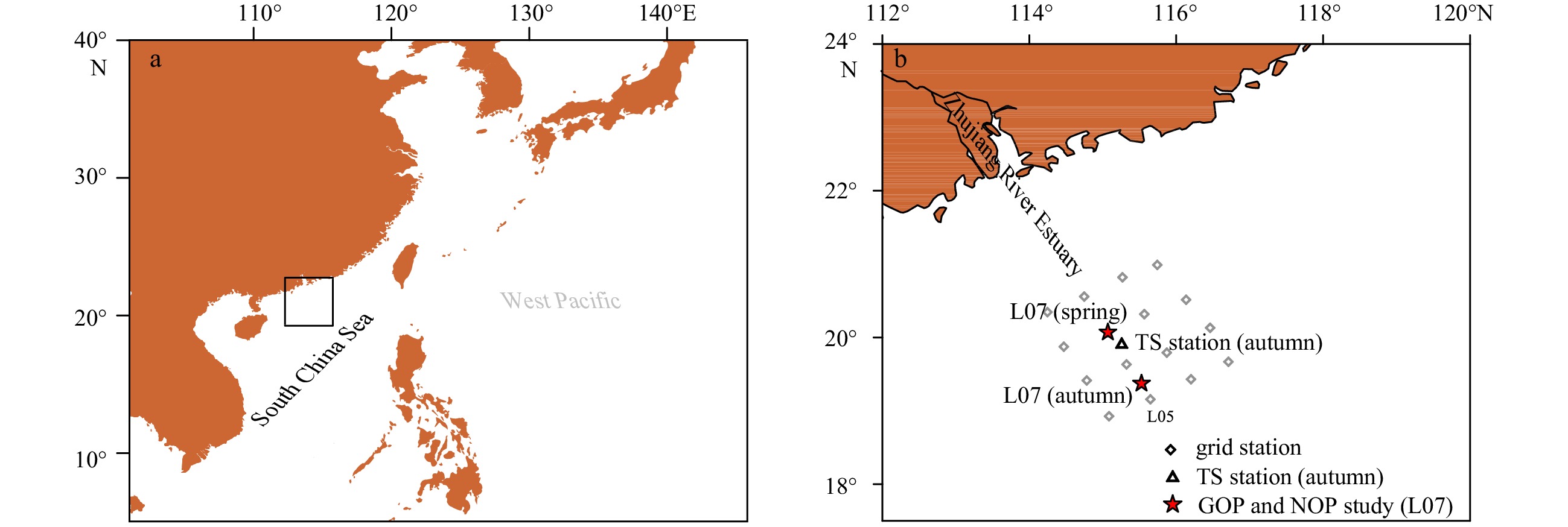
The South China Sea (SCS) is situated between the Tibetan Plateau and West Pacific Warm Pool, and includes shallow continental shelf waters (<200 m) in the north (Fig. 1a). In the northern SCS, upper water column ecosystem is impacted by the monsoon climate and occasional eddies. Primary production rates estimated by the ¹⁴C method reveal that in winter the primary and net production are usually higher relative to that in summer (Chen and Chen, 2006). Spatially, gross primary production and net community production show a seaward decrease (Wang et al., 2014). While cold (warm) eddies are usually thought to play a bigger (smaller) role in stimulating the upper water column ecosystem production, the exact positive or negative role is highly temporally and spatially related (Mahadevan et al., 2008). In the northern SCS, upwelling and hence increased primary production and export production has been observed at the edge of a warm eddy (Zhou et al., 2013).

Figure  1.  Study area (a) and sampling stations (b). In image a, the black box indicates the location of plot b. GOP represents gross oxygen production, NOP net oxygen production, and TS time series station.

DownLoad: Full-Size Img PowerPoint

Though the classic method (e.g., ¹⁴C) has been widely used for production calculations in the SCS (Ning et al., 2004; Chen and Chen, 2006; Chen et al., 2008; Song et al., 2012; Zhang et al., 2018), O₂ based methods are relatively limited (Wang et al., 2014; Huang et al., 2018; Hung et al., 2020). To the best of our knowledge, the triple oxygen isotope and O₂/Ar ratio method has not previously been applied in the SCS. Due to the contrasting time scales that classic ¹⁴C and triple oxygen isotope method respectively focuses (hours vs. weeks), it helps to achieve a comprehensive understanding of ecosystem production. Given the significant production seasonality and occasional eddies in the northern SCS, application of triple oxygen isotopes methods in the northern SCS ecosystem production assessment and a seasonal comparison are interesting. Furthermore, in spite of improvement in gas exchange term using 60 d time-weighted approach, the incorporation of 60 d history of mixed layer depth into it is not applied (Reuer et al., 2007). Hence, the contribution of using the mixed layer depth history in reducing the uncertainty in GOP and NOP remains unknown (Reuer et al., 2007).

Under this background, the questions in this work are: (1) by using the triple oxygen isotope and O₂/Ar ratio method, what is the seasonal production difference in the upper mixed layer in the northern SCS and its potential explanation; (2) to what extent the accuracy of the calculated production could be improved if the mixed layer depth history is reasonably reconstructed. To address this two questions, this study initially developed a model that could reasonably reproduce the mixed layer depth history (60 d prior to sampling) in the northern SCS. And then, the O₂/Ar ratio, ¹⁸O/¹⁶O ratio, and triple oxygen isotopes of the dissolved O₂ were measured in the upper 150 m at one station in the northern SCS slope region during two cruises; one in early summer/late spring (i.e., June, termed spring hereafter) and the other in autumn (October). These in situ techniques were used to determine gross primary production and net community production (as GOP and NOP, respectively) rates in the upper mixed layer. The GOP rate was first compared with diel O₂ concentration observations, and the production caveats and limitations were discussed. Improvements in GOP and NOP using the mixed layer depth history were then presented. Finally, the GOP rate was compared to that obtained with the classic ¹⁴C method (for October only), and both GOP and NOP results were compared and discussed in comparison with previously published rates. For samples beneath the mixed layer, the community respiration and nutrient regenerations from an oxygen isotope perspective was also discussed. The community respiration section is presented in the supplemental materials.

2. Materials and methods

The production rate was measured in terms of O₂ production and the GOP corresponds to the ¹⁴C based net primary production plus autotrophic respiration (Nicholson et al., 2012). The NOP corresponds to the net community production, which is the ¹⁴C based net primary production subtracted by the heterotrophic respiration. C and O₂ results can be converted using the C to O stoichiometry in each process.

2.1 Brief basis of the dissolved O₂ property method for measuring production

O₂ has three naturally occurring stable isotopes, ¹⁶O (99.76%), ¹⁷O (0.04%), and ¹⁸O (0.20%). The isotope composition of O₂ were presented using standard delta notation in units of per mil:

where ^*O can be either ¹⁷O or ¹⁸O. In this study, the standard was air, which by definition has a δ¹⁸O or δ¹⁷O value of 0‰.

The deviation in δ¹⁷O measured vs. expected based on the δ¹⁸O value of the sample was given using the Δ¹⁷O notation (Miller, 2002):

where λ is the reference slope and Δ¹⁷O is given in per meg (1 per meg = 0.001‰). For λ, this study used a value 0.518, which is the value slope observed during closed system respiration across a variety of microorganisms and animals (Luz and Barkan, 2005). Variations in Δ¹⁷O values in dissolved O₂ are thought to reflect the photosynthetic production of O₂ in the water column (Luz and Barkan, 2009). Δ¹⁷O values were previously used to calculate GOP in the mixed layer (Luz and Barkan, 2009). An alternative form of Δ¹⁷O was later provided by Prokopenko et al. (2011), which avoids mathematical approximations and therefore improves calculation precision (Prokopenko et al., 2011):

where [O₂]_eq is equilibrated O₂ concentration in the water; O_p and O_dis are the photosynthetically produced O₂ and dissolved O₂, respectively. In this study, GOP was calculated using Eq. (3), namely following Prokopenko et al. (2011).

NOP was calculated based on observed O₂ supersaturation in the water column due to biology. The O₂ supersaturation, ([O₂]/[O₂]_eq)_bio, was calculated based on the measured O₂ supersaturation in excess of Ar supersaturation, which accounts for bubble injection and physically induced changes in solubility:

where δ′(O₂/Ar) = (O₂/Ar)_measure/(O₂/Ar)_reference – 1, [O₂] is the measured O₂ concentration in the water. In addition to the O₂ supersaturation, this study followed the most recent NOP approach, namely further using the N₂O concentration in the mixed layer to calibrate for the mixing effect (Cassar et al., 2014):

where k is the O₂ or N₂O gas transfer velocity (m/d), [O₂]^B and [N₂O]^B are biological saturation concentrations of the respective gases, and ∂[O₂]^B/∂[N₂O]^B is the vertical gradient of [O₂]^B concentration to [N₂O]^B concentration. Within the mixed layer, [O₂]^B was defined as:

and [N₂O]^B was defined as:

where [N₂O] and [N₂O]_eq are the measured and equilibrated N₂O concentrations in the water, respectively. With respect to [N₂O]_thermal, which accounts for solubility changes resulting from recent heat flux in the surface water, it was calculated as (Izett et al., 2018):

where Q is heat flux (W/m² or J/(m²·s)), c_p is heat capacity (J/(kg·C)), ρ is seawater density (kg/m³), and T is temperature. The number 86400 is the coefficient transforming time unit from day to second. The negative operator converts the Q and positive c_p into a sea-to-air N₂O flux (Izett et al., 2018). To achieve the same time scale as the time-weighted approach for the gas exchange term (i.e., 60 d) (Reuer et al., 2007), the [N₂O]_thermal was the mean value over 60 d before the sampling time. The heat flux Q history was obtained from a previous comprehensive study of the Q history in the SCS (Liu et al., 2020). The heat capacity c_p is a function of temperature and salinity. In this study, the exact c_p was calculated based on the sea surface temperature (SST) history (60 d prior to sampling), which was downloaded from the Remote Sensing Systems database (www.remss.com) and the salinity was regarded as unchanged since it plays a very limited role in determination of the c_p value. In the water beneath the mixed layer, no thermal correction for N₂O was conducted (i.e., [N₂O]_thermal = 0 in Eq. (8)) (Izett et al., 2018). Also note that the N₂O calibration approach assumes that lateral advection has very limited impact on N₂O concentration in mixed layer.

We calculated the expected value of dissolved O₂ and Ar in equilibrium with the atmosphere using the solubility equations given in Garcia and Gordon (1992) based on measured seawater temperatures and salinities. The equilibrated N₂O (i.e., [N₂O]_eq) was calculated at a given temperature and salinity according to the equation presented by Weiss and Price (1980). [N₂O] data was obtained from a previous study (Zhang et al., 2019a). Within the mixed layer, N₂O data in June corresponded well to O₂ data of this study in all layers and hence all layers of NOP calculations were calibrated for the vertical mixing effect via the N₂O approach. Regarding October, however, N₂O data was only available in the surface layer (5 m) and therefore the N₂O based calibration was only conducted for the surface layer in October, and not for the remaining deeper layers.

Finally, the gas exchange term (k in Eqs (3) and (5)) was calculated following the time-weighted approach given by Reuer et al. (2007), in which the mixed layer depth history is further obtained via numerical modeling. This is described further in Section 2.3.

2.2 Field sampling and laboratory analyses

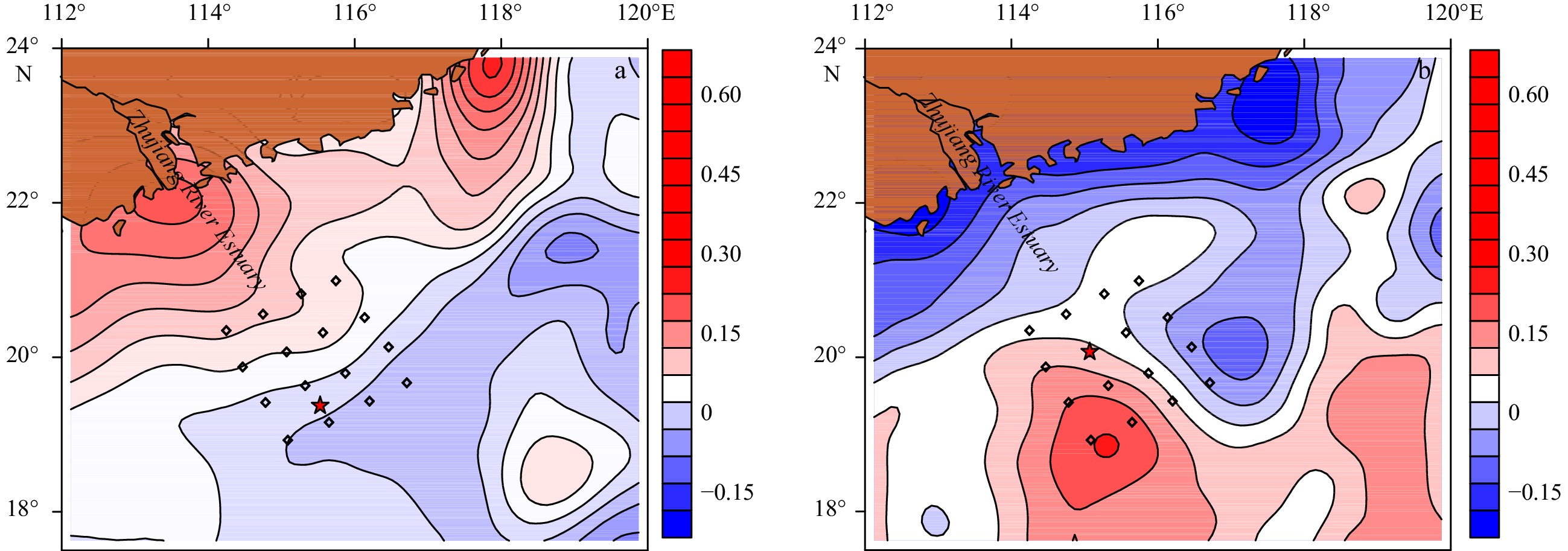
Two cruises were conducted in the slope region of the SCS on the R/V Nanfeng. The first cruise occurred in October 2014 (autumn) and the second in June 2015 (spring). Initially, 16 grid stations were sampled for surface (3−5 m) temperature and salinity measurements (Fig. 1b). Station L07, which was within the grid station coverage, was selected in both cruises for the triple oxygen isotopes and O₂/Ar ratio study. Discrete water samples in the upper 150 m at Station L07 were collected via a Niskin sampler. The Station L07 location in both seasons was not constant. The autumn and spring Station L07 locations differed by 90 km, with the station in spring closer to the mainland and the Zhujiang River Estuary (Fig. 1b). However, both stations had water depths over 500 m. In autumn, an additional station, time series station, was monitored for 25 h (beginning at 7:00 pm on October 26, 2014), with water samples at 5 m depth collected at roughly 3 h intervals to determine the O₂/Ar ratio. ¹⁴C incubations were conducted at the identical station (L07) for the autumn cruise (October 2014), whereas for the spring cruise, the nearest ¹⁴C incubation was carried out at Station L05 (Fig. 1b). Discrete water samples were collected via Niskin bottles mounted on the CTD rosette. A cyclonic-anticyclonic eddy pair occurred around the O₂ sampling Station L07 in June (Chen et al., 2016), and Station L07 was on the edge of the anticyclonic eddy, as deemed by the sea level anomaly (Zhang et al., 2019a). In October, no eddies occurred in the grid stations during sampling.

Depth profiles of temperature, salinity, and fluorescence were measured using a CTD (Seabird 9). Secchi disk readings were used to measure the euphotic zone depth (the depth where 1% of the surface photosynthetically available radiation remains). In addition, in June 2015, a photosynthetically available radiation sensor, which measures irradiance, was also included on the CTD rosette to provide additional calibrations for the Secchi disk measurements.

With respect to the ¹⁴C incubations for primary production, the euphotic zone depth was first measured by the photosynthetically available radiation sensor (or calculated from the Secchi disk depth) onboard, then the six depths were calculated according to the light attenuation (100%, 50%, 30%, 10%, 5%, and 1%). The ¹⁴C incubations were performed in three samples at each depth; there were 250 mL samples incubated with 10 μCi sodium bicarbonate (NaH¹⁴CO₃) for 4–6 h, following the Joint Global Ocean Flux Study protocols (Knap et al., 1996). Samples were filtered through a 200 μm nylon mesh. The ¹⁴C-P (¹⁴C-based primary production) values were derived from the 4–6 h incubations linearly extrapolated to 12 h. The discrete ¹⁴C-P values were trapezoidally integrated to yield an integrated production value at a given water column thickness.

For triple oxygen isotope and O₂/Ar ratio measurements, there were 250 mL water samples collected into 500 mL glass bottles, with side arms sealed by an O-ring-seated valve following methods outlined in Reuer et al. (2007) and references therein. Following this, O₂ and Ar were purified for measurements in the laboratory (within 10 months after sample collection): the majority of the water was pumped out under vacuum. The remaining few milliliters of seawater were frozen at −40°C in an ethylene glycol and water mixture. H₂O, CO₂ and N₂ were removed by cryogenic trap and an automated gas chromatographic system as described in Blunier et al. (2002). O₂ and Ar were collected by molecular sieve at liquid nitrogen temperature. After heating at 100°C for 1 h, the trapped O₂ and Ar were introduced into a dual inlet mass spectrometer (Thermo-Finnigan DELTA Plus XL). Based on laboratory standards (mercury-chloride-poisoned deionized water equilibrated with air) analyzed during the 1 month analytical period (n=5), the precisions (±1 standard deviation) of δ¹⁷O, δ¹⁸O, and δO₂/Ar were 0.011‰, 0.022‰, and 0.68‰, respectively. The precision of Δ¹⁷O was 11 per meg (±1 standard deviation). The triple oxygen isotopes and Ar measurements were all done in the oxygen gas isotope lab in Princeton University.

For measurements of dissolved inorganic nutrients (${{\rm {NO}}_3^-} $, ${{\rm {SiO}}_3^{2-}} $, and ${{\rm {PO}}_4^{3-}} $), seawater samples were filtered via acid-cleaned acetate cellulose filters. Mercury chloride was added into the water samples to kill all living organisms. Nutrient samples were stored at 4°C in the dark until analysis in the laboratory. Dissolved inorganic nutrient values were measured photometrically using an auto-analyzer (SEAL Analytical, AA3) with a precision (±1 standard deviation) greater than 3%. Nutrient values for June 2015 were published previously (Zhang et al., 2019a).

The propagated errors of laboratory precision measurements were estimated using the Monte Carlo approach (Quay et al., 2010; Munro et al., 2013; Haskell II et al., 2017), with slight modifications. For GOP, this study calculated the GOP rate in both seasons (October and June) following Eq. (3), with 100 000 simulations of randomly selected values for δ¹⁷O, δ¹⁸O, and k within the uncertainty estimated for each variable. The upper and lower bounds for GOP were then calculated as one standard deviation from the best estimate (which is also the mean), determined as the percentile between 16% and 84% of the simulated production rates, and this was reported as the error in GOP. The program was independently run at least three times to confirm that the standard deviations varied by less than 4.5%. Uncertainties for δ¹⁷O and δ¹⁸O were 0.011‰ and 0.022‰, respectively, and the uncertainty of k was 13.5% (Bender et al., 2011). In addition, similar procedures were carried out to obtain the propagated errors in NOP, and α in the mixed layer.

2.3 Gas flux parametrizations and mixed layer depth history calculations

The piston velocity, k in Eqs (3) and (5), was calculated following a time-weighted approach as proposed by Reuer et al. (2007), which requires 60 d of SST, wind speed, and mixed layer depth history prior to the sampling date. In brief, for the previous 60 d, the k at each day (k_i) is a function of wind speed and Schmidt number (Sc number) of that day, which can be quantified via the equations of Sweeney et al. (2007). When the 60 k_i values (i ranges from 1 to 60) are pooled together to calculate a time-weighted k (which is used in Eqs (3) and (5)), the mixed layer history of the 60 d is used, which helps quantify the individual k_i contribution to the final k (Reuer et al., 2007). To calculate $k_{{\rm{O}}_2} $ and $k_{{\rm{N}}_2{\rm{O}}} $, the respective Sc number is calculated according to O₂ or N₂O gas parameters (Wanninkhof, 1992), and the daily SST is used to improve the Sc number precision on that day.

In order to reconstruct the mixed layer history, the Hybrid Coordinate Ocean Model was used to reconstruct the temperature and salinity profile in Station L07, analyzing data with (1/12)° horizontal resolution and a 1 d time resolution (https://hycom.org/dataserver/gofs-3pt0/analysis). The surface forcing of the Hybrid Coordinate Ocean Model included wind stress, wind speed, heat flux, and precipitation. It also used the Navy Coupled Ocean Data Assimilation system to assimilate satellite altimeter data, SST, and CTD profiles from XBTs, ARGO floats, and moored buoys. The temperature and salinity data interpolated vertically to 1 m resolution; therefore, the vertical density resolution is 1 m. The mixed layer depth for 60 d before the sampling date was then reconstructed from the model time series of density vs. depth. The mixed layer depth was the shallowest depth where the density was greater, by 0.125 kg/m³, than the density at the surface.

The wind speed data (derived from signals of the scatterometer as an estimate of wind speed 10 m/s above the sea surface), as well as SST for the 60 d prior to the sampling time, were downloaded via the database of Remote Sensing Systems (www.remss.com).

3. Results

3.1 Physical parameters during the sampling months

The physical parameters in both June and October have been previously described (Chen et al., 2016; Zhang et al., 2019a, b). Briefly, the surface salinity of all grid stations in June 2015 was lower than that in October 2014 (mean 33.90 in October vs. 33.17 in June) and a lower surface salinity was also found at Station L07 in June relative to October (33.80 in June vs. 34.06 in October; Table 1). As indicated by a water belt with a salinity less than 32, a stronger terrestrial impact on the slope area in June was expected relative to October (Fig. 2). Furthermore, in June, the slope region was under the influence of a pair of cyclonic and anticyclonic eddies, while no mesoscale processes were detected in October 2014 (Chen et al., 2016; Zhang et al., 2019a). As indicated by the sea level anomaly, Station L07 was on the edge of the anticyclonic eddy (Fig. A1), which was in the vicinity of a submesoscale upwelling (Chen et al., 2016).

Table  1.  Main physical parameters in spring (June) and autumn (October) in the present study

Parameter	Spring	Autumn
Mixed layer depth/m	21.5	39.5
k (time-dependent)*/(m·d–1)	2.524	7.485
k′ (time-independent)/(m·d–1)	2.285	7.509
SST/°C	30.208	26.957
Salinity	33.808	34.061
[O2]eq/(μmol·L–1)	195	205
([O2]/[O2]eq)bio	1.0111	1.0009
GOP/(mmol·m–2·d–1) (by O2)	189±26	169±23
NOP/(mmol·m–2·d–1) (by O2)	8.2±1.1	1.5±0.7
GOP/14C-P	–	5.4
Note: GOP, gross oxygen production; NOP, net oxygen production; k, pooled piston velocity; [O2] and [O2]eq represent the measured and equilibrated O2 concentration in the water, respectively; 14C-P represents 14C-based primary production; – represents no data; * this value was considered in the final GOP calculation.

 | Show Table

DownLoad: CSV

Figure  2.  Surface salinity distribution in October 2014 (a) and June 2015 (b) as revealed by grid stations (diamonds). The red star indicates the location of Station L07 where O₂ samples were collected. Note that salinity ranges and gradients in both seasons are the same.

DownLoad: Full-Size Img PowerPoint

3.2 Meteorological history for Station L07

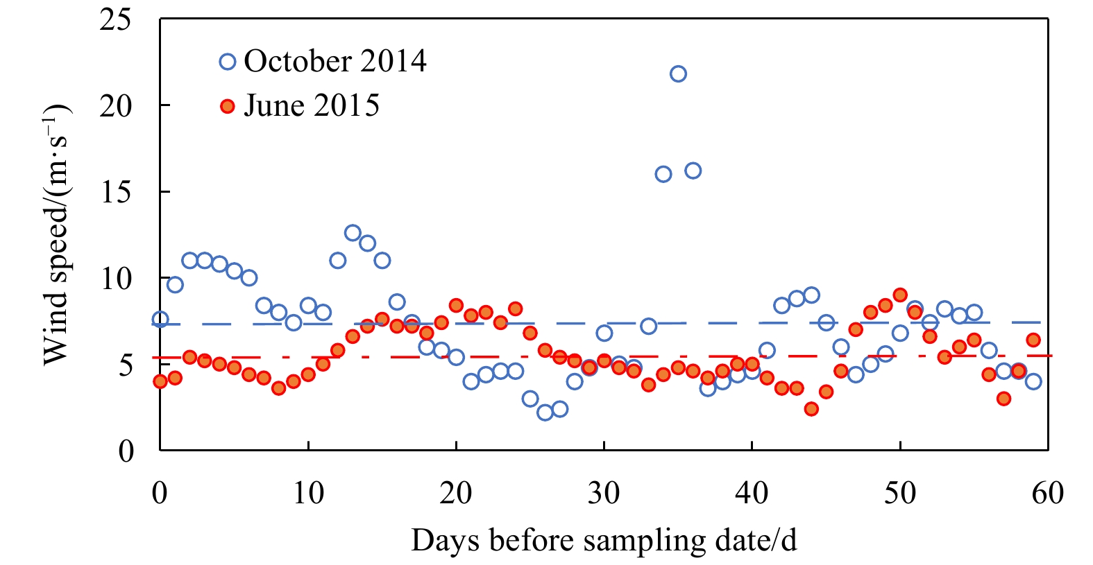
In open sea, although water column stead state is usually not required in GOP and NOP studies, meteorological history is essential in improvement of GOP and NOP calculation. For the 60 d prior to sampling, the average wind speed at the study site was 7.4 m/s (2.2–21.8 m/s) in October 2014, and 5.6 m/s (2.4–9 m/s) in June 2015 (Fig. 3). Note that in the period from approximately 15 d to 25 d prior to the June sampling date, the station endured a high-wind-event (Fig. 3). SST during the 60 d prior to our sampling ranged from 25.80°C to 30.75°C in 2014 and 25.20°C to 30.30°C in 2015. The 60 d mixed layer depth history indicates that the mixed layer depth in both seasons had become shallower in the recent weeks, and such a trend was especially severe in October (Fig. 4).

Figure  3.  Wind speed before the sampling date (0 d is the sampling date). The blue dashed line (7.4 m/s) indicates the mean wind speed of the 60 d for observation in 2014 and the red dashed-dot line (5.6 m/s) indicates that for 2015. Data derived from www.remss.com.

DownLoad: Full-Size Img PowerPoint

Figure  4.  Modeled mixed layer depth history until the sampling date (a. October 2014; b. June 2015). The observed mixed layer depth at the sampling date is shown as the red asterisk on the right y axis. The black dashed line indicates 5 d (a) and 8.5 d (b) before the sampling date, which gets close to the O₂ residence time within the mixed layer. The bottom layer of the mixed layer criteria is a 0.125 kg/m³ difference from the surface. Note that the x-axis is reverse in direction relative to Fig. 3.

DownLoad: Full-Size Img PowerPoint

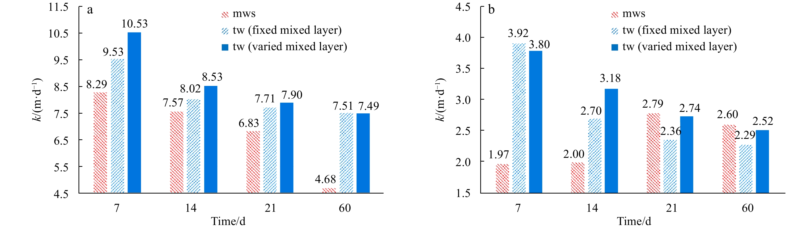
The calculated time-weighted value for k was 7.49 m/d in autumn and 2.52 m/d in spring (Table 1). As a comparison, k values based on other approaches were also calculated, including k′ based on the time-weighted method, but the mixed layer depth remained constant for the entire 60 d. k″ was also calculated based on the mean wind speed method (Fig. 5); it decreased from 8.29 m/d (7 d mean) to 4.68 m/d (60 d mean) in October 2014 and increased from 1.97 m/d (7 d mean) to 2.60 m/d (60 d mean) in June 2015. The time-weighted methods yielded values (k and k′) that followed the same trend in both seasons, namely a decrease with increasing number of days (Fig. 5) and was more stable when time-weighted days exceeded 21 d (Fig. 5).

Figure  5.  Pooled piston velocity k values in October 2014 (a) and June 2015 (b). mws, mean wind speed method (k″ in the text); tw (fixed mixed layer), time-weighted method with mixed layer unchanged (k′ in the text); tw (varied mixed layer), time-weighted method with mixed layer changed. Note that 7.49 and 2.52 were accepted as the k value in calculating the gross oxygen production for October 2014 and June 2015, respectively, and the x axis is disproportional.

DownLoad: Full-Size Img PowerPoint

3.3 Profile observations at Station L07 in June 2014 and October 2015

In both seasons, ([O₂]/[O₂]_eq)_bio decreased from the surface to 150 m depth (Figs 6a and c). The mixed layer ([O₂]/[O₂]_eq)_bio was lower in autumn compared with that in spring (1.000 9 vs. 1.011 1). However, in deeper waters (larger than 100 m), ([O₂]/[O₂]_eq)_bio in spring was lower compared with that in autumn (0.618 5 vs. 0.686 4; Figs 6a and c). Dissolved O₂ δ¹⁸O values in the mixed layer were lower in the shallower samples compared with in the deepest samples (Figs 6a and c). Shallow water (depths of 0–80 m) autumn Δ¹⁷O values were lower compared with those in spring (Figs 6a and c). Specifically, average Δ¹⁷O values within the mixed layer were 24 per meg in autumn (n=3) and 54 per meg in spring (n=1). Elevated Δ¹⁷O values were observed at depths between 50 m and 80 m in spring, whereas in autumn the depth interval of elevated Δ¹⁷O values was between 50 m and 100 m (Figs 6a and c).

Figure  6.  O₂ properties (δ¹⁸O, ([O₂]/[O₂]_eq)_bio, and Δ¹⁷O in per meg), ${{\rm {NO}}_3^-} $ concentration (μmol/L), and fluorescence signal at Station L07 in October 2014 (a, b) and June 2015 (c, d). The illumination condition is shown by dashed lines, PAR represents photosynthetic active radiation.

DownLoad: Full-Size Img PowerPoint

In spring, the depth of the euphotic zone (1% light level) was 79 m, with the 0.1% light level occurring at 117 m depth (Fig. 6d). In October 2014, the euphotic zone depth was 56.9 m (Fig. 6b). The fluorescence signal showed peaks at the bottom of the euphotic layer in both seasons (Fig. 6d). Nitrate remained depleted in the upper 40 m during autumn and upper 60 m during spring. In the deeper waters (larger than 100 m), nitrate concentrations were similar between both seasons (Figs 6b and d).

3.4 Time series observations in autumn (October 2014)

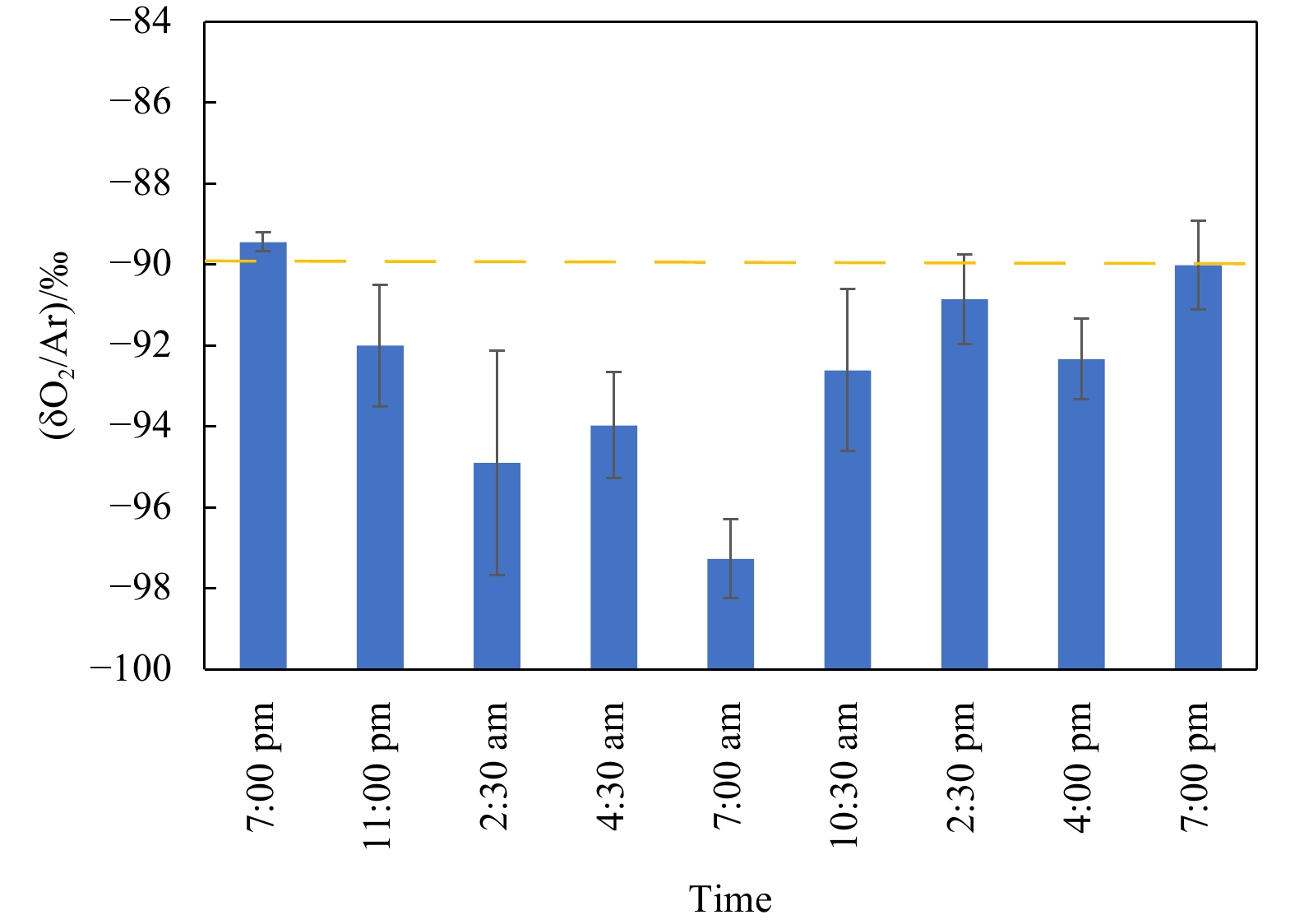
The mean temperature and salinity at time series station were 27.29 °C and 33.74, respectively, and showed limited variability during the 25 h period in the diel cycle observed. Based on this, the expected δO₂/Ar ratio value for dissolved gas in equilibrium with the atmosphere was –90.87‰. During the night (7:00 pm to 7:00 am), [O₂] decreased with time as indicated by the decreasing δO₂/Ar (Fig. 7). During the day, δO₂/Ar ratio increased from –97.27‰ at 7:00 am to –90.02‰ at 7:00 pm (Fig. 7). With respect to the ([O₂]/[O₂]_eq)_bio value, it was 1.001 3 at 7:00 pm (night of 26 October), decreased to 0.992 7 at 7:00 am (morning of 27 October), and then increased to 1.000 6 at 7:00 pm (evening of 27 October).

Figure  7.  δO₂/Ar values plotted against time at 5 m depth of the time series station. Note that the x axis is disproportional.

DownLoad: Full-Size Img PowerPoint

4. Discussion

4.1 Caveats and limitations in NOP and GOP estimations

Based on the triple oxygen isotope data, at Station L07, GOP in spring and autumn were (189±26) mmol/(m²·d) (by O₂) and (169±23) mmol/(m²·d) (by O₂), respectively (Table 1). The NOP in spring and autumn were (8.2±1.1) mmol/(m²·d) (by O₂) and (1.5±0.7) mmol/(m²·d) (by O₂), respectively (Table 1).

Regarding the NOP, the vertical mixing effect between the mixed layer and layers beneath was calibrated via a N₂O based approach (Eq. (5)) (Cassar et al., 2014), with the gas flux parametrization refined via a time-weighted approach (Reuer et al., 2007). However, the potential nitrification process within the mixed layer and its impact on the NOP estimate, which is extensively discussed in a previous publication (Izett et al., 2018), was not applied in this study due to lack of nitrification rate data. As suggested by the previous authors, the consideration of potential nitrification within the mixed layer likely plays a minor role in contributing uncertainties to the final NOP compared with other error sources such as gas transfer parameterizations (Izett et al., 2018). If the vertical mixing was ignored and only the gas exchange term was considered (i.e., the latter part in the brackets in Eq. (5) was ignored), the vertical mixing non-calibrated NOP was 1.5% to 9.5% lower than the current vertical mixing calibrated NOP result (Table 1). This difference (1.5% to 9.5%) is at the lower end when compared with that reported in the subarctic northeast Pacific (0.3% to 42%) (Izett et al., 2018). With respect to GOP, no calibration was applied to account for the vertical mixing. Therefore, this could be the largest source of uncertainty in our reported GOP values (Table 1). However, potential deviation in our estimated GOP can be judged through a comparison with the diel O₂ observation results, which are discussed below.

Within the euphotic zone, respiration and photosynthesis occur during the day while only respiration occurs at night. If this study assumes that the respiration rates in the day and night are equal and that no significant vertical water exchange occurs within the 24 h, then GOP can be independently estimated based on the O₂ budget in the mixed layer as follows:

where Δ[O₂]_day (mmol/m³) is the O₂ increase during the day; Δ[O₂]_night (mmol/m³) is the O₂ decrease during the night; N is the mixed layer thickness. It should be noted that here this study assumes the lateral current induced very limited (or trace) effect to GOP. This is likely the case as the horizontal [O₂] distribution usually is the same within a very limited area in the open sea.

Here, Δ[O₂] is calculated from the measured δO₂/Ar value, assuming that Ar concentrations are in equilibrium with gaseous Ar in the atmosphere:

where ${R_{({{\rm{O}}_2}{/{\rm{Ar}}){\rm{air}}}}} $ is the ratio of O₂ to Ar in the air (22.43). δ(O₂/Ar)_initial and δ(O₂/Ar) _final are the initial and final δ(O₂/Ar) values (in per mil) at time series station, respectively (Fig. 7).

This study notes that the observation time (26 or 27 October, 2014) is close to the Autumnal Equinox (23 September), and given the subtropical location, the day and night lengths are similar (11.5 h vs. 12.5 h). Therefore, although the respiration rate remains unclear, the respiration times for day and night are very similar. This study assumes that respiration contributes equally between day and night in the diel observations.

Using Eqs (9) and (10), the GOP for autumn was estimated at 134 mmol/ (m²·d) (by O₂) based on the diel observation. Given the propagated error, these two values (134 mmol/(m²·d) (by O₂) vs. (169±23) mmol/(m²·d) (by O₂) as estimated by triple oxygen isotopes method, Table 1) critically are not in agreement with each other. This is largely due to the uncertainties originating from the vertical mixing in the water column that results in overestimates of the GOP via the triple oxygen isotope method. If the diel observation result is regarded as vertical mixing impact free (134 mmol/(m²·d) (by O₂), then the vertical mixing impact to the triple oxygen isotope GOP is 26% (134 mmol/(m²·d) (by O₂) vs. 169 mmol/(m²·d) (by O₂)). In previous triple oxygen isotopes GOP studies, overestimation due to vertical mixing is estimated to be as high as 60% to 80% (Nicholson et al., 2012). Further research is needed to further quantify the vertical mixing effect. This study notes that this exercise (diel O₂ budget calculation for GOP) could not be repeated for the spring cruise in 2015 because water column diel samples were not collected.

4.2 Application of mixed layer depth history in gas flux parametrizations

Estimates of GOP and NOP require knowledge of the mixed layer depth prior to the sampling date. However, usually the mixed layer depth is only known for the sampling date. The mixed layer depth history was reconstructed using a modeling approach. This study checked the accuracy of the model by comparing the measured mixed layer depth vs. the modeled mix layer depth on the sampling date. Specifically, our modeled mixed layer depths for the autumn and spring sampling dates were 38 m and 16 m, respectively. In comparison, the observed mixed depths for autumn and spring on the sampling dates were 39.5 m and 21.5 m, respectively. Our modeled and measured mixed layer depths were similar (within 1.5 m for autumn and 6 m for spring), indicating acceptable model results.

Gas exchange plays a key role in determining final production (Haskell II et al., 2017), and it is usually one of the main sources of uncertainty in the calculation of production (Stanley et al., 2010). The mean wind speed method is not recommended because k″ did not show a clear variation pattern with increasing number of days in both seasons (Fig. 5). For the time-weighted approach, the period considered should be at least over 14 d, but 60 d is the optimal because the k values showed a sharp decrease in the first 2 weeks and remained more stable when the period exceeded 21 d (Fig. 5). The k′ at 60 d (time-weighted but mixed layer depth unchanged) was 7.509 m/d in autumn and 2.285 m/d in spring (Table 1, Fig. 5). Based on the modeled mixed layer history, the calculated difference in time-dependent k vs. time-independent k′ was 0.3% in October 2014 and –9.5% in June 2015 (Table 1).

Given that the potential vertical mixing would introduce a 26% error (see Section 4.1), the mixed layer depth history only reduced a minor portion of the error (maximum 9.5%). Therefore, if no numerical model for mixed layer depth history is available in a production study, the mixed layer depth history is considered unnecessary, instead a previously recommended time-weighted approach for k is sufficient (Reuer et al., 2007).

4.3 ¹⁴C index for production comparison

The ¹⁴C-P rate versus depth profile is shown in Appendix (Fig. A2). The photosynthetic quotient (PQ) reflects the stoichiometry of O₂ generation and C fixation in photosynthesis (Laws et al., 2000). Compared with our estimated GOP (Table 1), this corresponds to a GOP/¹⁴C-P ratio (O₂/C molar ratio), i.e., a PQ value of 5.4 in autumn. It is not unexpected that the PQ was larger than 1, as GOP is the gross production and ¹⁴C-P is the net production, which differs in autotrophic respiration. The PQ value of 5.4 in autumn was higher than that reported in previous studies. For example, the GOP/¹⁴C-P ratio was 2.7 (O₂/C molar ratio) in the same incubation experiment (Marra, 2002); GOP was estimated using an ¹⁸O tracer. Other studies reported a GOP/¹⁴C-P value of around 2.2 (with GOP estimated using Δ¹⁷O values), which is close to 2.7 (e.g., Quay et al., 2010), while the ratio was found to be 7.9 and 7.6 in the Bermuda Atlantic time series study and a study at Lake Kinneret (Israel), respectively (Luz and Barkan, 2009). In the Western Equatorial Pacific, the ratio was reported to be as high as 8.2 (Stanley et al., 2010). More recently, based on monthly observations, Nicholson et al. (2012) used a model to exclude an entrainment effect in GOP estimates and found the GOP/¹⁴C-P ratio to be 2.6 in the Bermuda Atlantic time series study and 1.4–3.0 at the Hawaii Ocean time-series station in the subtropical Pacific. Given the potential entrainment effect due to the complex mixed layer depth history at the study site (Fig. 4a) and the elevated production below the mixed layer (Fig. A2a), the reported GOP/¹⁴C-P ratio and GOP results (Table 1) should be considered the upper limits.

4.4 Implications for the SCS production

Production in the SCS has been intensively studied (Ning et al., 2004; Chen and Chen, 2006; Song et al., 2012; Huang et al., 2018; Hung et al., 2020), most of the research has been based on ¹³C, ¹⁴C or ¹⁵N methods. The reported values have generally been based on an euphotic zone integration. Winter is usually a more productive season relative to spring/summer, and there appears to be a large variation in IPP (integrated primary production) and INP (integrated net production) values (Table 2) both spatially and temporally in the shelf and slope region (Chen, 2005). For the shelf break and slope region close to our study area, the euphotic-zone-integrated IPP showed a large variation, ranging from 19 mmol/(m²·d) (by C) to over 75 mmol/(m²·d) (by C) (Table 2). The euphotic zone integrated ¹⁴C-P result (411 mg/(m²·d) (by C) in autumn and 373 mg/(m²·d) (by C) in spring; or 34 mmol/(m²·d) (by C) in autumn and 31 mmol/(m²·d) (by C) in spring are within the previously reported ranges (Table 2).

Table  2.  Pooled production rates for the SCS shelf/slope region and other subtropical regions

Date	INP/(mmol·m–2·d–1) (by C)	IPP/(mmol·m–2·d–1) (by C)	Region	Data Source
Jul./Aug. 2006	–	>75	–	Song et al. (2012)
Jul. 2003, Jun./Jul. 2004	5–14	68.0–72.5	SCS shelf and slope regions	Chen and Chen (2006)
Oct. 2002	2.5–18	12.5–51.0	SCS shelf region	Chen (2005)
May 2005	–	27	SCS basin region	Zhang et al. (2018)
Jun./Jul.1998	–	19	SCS basin region	Ning et al. (2004)
Oct. 2014	–	34	–	present study
Jun. 2015	–	31	–	present study
Oct. 2014	1.5±0.7	169±23	SCS slope region	present study
Jun. 2015	8.2±1.1	189±26	SCS slope region	present study
Aug. 2012	0–50	200	SCS slope region	Wang et al. (2014)
July	–	270–376	SCS shelf edge	Hung et al. (2020)
Annual	10.7	–	SCS basin	Huang et al. (2018)
Annual	14±4	50–240	subtropical Pacific	Quay et al. (2010)
Aug. to Sep. 2006	5.9±0.9	121±34	western equatorial Pacific	Stanley et al. (2010)
Annual	6–8.3	29–103	BAT	Luz and Barkan (2009)
Annual	–	0–280	BAT	Nicholson et al. (2012)
Annual	–	25–210	HOT	Nicholson et al. (2012)
Note: BAT, Bermuda Atlantic time series study; HOT, Hawaii Ocean time series study; INP, integrated net production; IPP, integrated primary production; SCS, South China Sea; –, no data.

 | Show Table

DownLoad: CSV

In addition to the above widely applied methods, the O₂ concentration based method has also been utilized (Wang et al., 2014; Huang et al., 2018; Hung et al., 2020). Based on the black and white bottle O₂ concentration method, Wang et al. (2014) found that the NOP varied strongly in the northern SCS in July or August, with the NOP and gross primary production of the slope region less than 0 to 10 mmol/(m²·d) (by O₂) and 200 mmol/(m²·d) (by O₂), respectively. More recently, Hung et al. (2020) using a similar black and white bottle O₂ concentration method reported a slightly higher GOP rate in the northern SCS, which in July was 270–386 mmol/(m²·d) (by O₂). However, this study was also based on an euphotic zone integration (much deeper than the mixed layer in July) (Hung et al., 2020), and their station (Station I) was considerably closer to the mainland, with a shallower water depth (between 100 m to 200 m) relative to the slope region with a depth exceeding 500 m (Fig. 1b). These reported GOP and NOP rates are comparable with our reported GOP (169–189 mmol/(m²·d) (by O₂)) and NOP (1.5–8.2 mmol/(m²·d) (by O₂)) values (Table 1).

Further offshore in the SCS basin, Huang et al. (2018) used a O₂ mass balance method, and Ar and O₂ data to yield a SCS basin annual net bio-generated oxygen flux (i.e., NOP) of 10.7 mmol/(m²·d) (by O₂), which was calculated to the deepest winter mixed layer depth of 56 m. This is slightly higher compared with our reported seasonal NOP value of (8.2±1.1) mmol/(m²·d) (by O₂) (June) and (1.5±0.7) mmol/(m²·d) (by O₂) (October) within the mixed layer depth of 21.5–39.5 m (Table 1).

Direct production measurements and further surface seawater pCO₂ determination indicate that production in the slope region of northern SCS (i.e., our study area) is usually higher in October than in June (Liu et al., 2002; Chen, 2005; Li et al., 2018, 2020; Hung et al., 2020). However, the GOP and NOP values recorded in June showed the reverse trend, namely higher GOP and NOP in June relative to that in October (Table 1). Regarding GOP, this may be partially due to the vertical mixing process and entrainment effect, which was not calibrated (Table 1). However, for NOP, in which the vertical mixing and entrainment effect were calibrated (Eq. (5)), it indeed showed a higher value in June compared with that in October (Table 1). This June-high and October-low pattern is consistent with the observed ([O₂]/[O₂]_eq)_bio value, as a higher ([O₂]/[O₂]_eq)_bio value was recorded in June relative to October (Fig. 6).

On the one hand, it has been found that eddies have a complex impact on marine ecosystem, which is highly temporal and spatial heterogeneous (Zhou et al., 2013), and in June our observation station was located close to the edge of an anticyclonic eddy (Fig. A1b) (Chen et al., 2016; Zhang et al., 2019a). Although common downwelling exists in anticyclonic eddy centers, the edge area is very productive due to submesoscale upwelling (Zhou et al., 2013). This finding (Zhou et al., 2013) supports the abnormally high production in June (Table 1) relative to October when no eddy occurred. On the other hand, the surface salinity distribution indicated a stronger terrestrial impact in June compared with in October in the slope area of northern SCS (Fig. 2). A lower salinity at Station L07 in June compared with October was also recorded (33.8 in June vs. 34.1 in October). The possible mechanism includes the occurrence of the eddy pair in June, which enhanced mesoscale lateral advection, and hence resulted in a more efficient cross-shelf transport (Zhang et al., 2019a). In the northern SCS, higher GOP and NOP production is repeatedly found in the region under stronger terrestrial impact, whereas in offshore open ocean waters, such production is usually much more depleted (Wang et al., 2014; Hung et al., 2020). The abnormal higher production in June compared with that in October warrants further study.

5. Conclusions

The triple oxygen isotope methods and O₂/Ar methods have been applied to the study of marine production for 20 a, which is much shorter in timeframe compared with the classic ¹⁴C based index. Such O₂ indices are incubation free and can be conducted in grid station investigations without having to consider the nighttime issue. These indices are hence an important supplement to the current ¹⁴C based index for improved ecosystem monitoring and assessment.

A series of modifications have been applied to improve the O₂ budget consideration in order to increase the precision of the final GOP and NOP. As one of the biggest error sources, the gas exchange term, k, greatly determines the precision of the estimated GOP and NOP. In addition to the time-weighted approach, as presented by Reuer et al. (2007), a consideration of the mixed layer depth history for the 60 d further helps improve k precision by reducing the error by up to 9.5% in the northern SCS. This error is much lower than other error sources (e.g., 26% uncertainty with vertical mixing); however, a knowledge of the mixed layer depth history is required.

With this improvement, based on the consideration of mixed layer depth history, this study reported the GOP and NOP rates in the SCS slope region (Station L07) for the first time, to the best of our knowledge. While the vertical mixing effect on NOP was calibrated via the latest N₂O based approach, the vertical mixing effect was not calibrated for GOP. However, a comparison with diel observation indicates a 26% overestimation in the current GOP value. This study reported values are consistent with previously reported production values in this region, which were based on the classic O₂ concentration method. While the eddy effect and terrestrial impact likely play a role, additional work is needed to further explain the abnormal monthly production pattern between June and October at this study site.

Acknowledgement

We acknowledge the captain and crew of R/V Nanfeng for their assistance in the field work. We thank Michael Bender and Jason Cutrera from Princeton University who helped us with lab work. We thank Daniel Stolper from Princeton University (now in University of California, Berkeley) who measured part of the samples, and further helped us with lab work. We thank W. J. Zheng, who helped us with water sampling in the field.

A1.  Sea level anomaly (m) on October 13, 2014 (a) and June 15, 2015 (b) in this study. Note that both plots share the same contour range and color scale. Star indicates Station L07. Sea level anomaly data downloaded from https://las.aviso.altimetry.fr/las/.

DownLoad: Full-Size Img PowerPoint

A2.  ¹⁴C-P rate versus depth within the euphotic zone in autumn (Station L07, mixed layer depth of 39.5 m) and spring (Station L05, mixed layer depth of 27 m). The dashed line indicates the bottom of mixed layer.

DownLoad: Full-Size Img PowerPoint

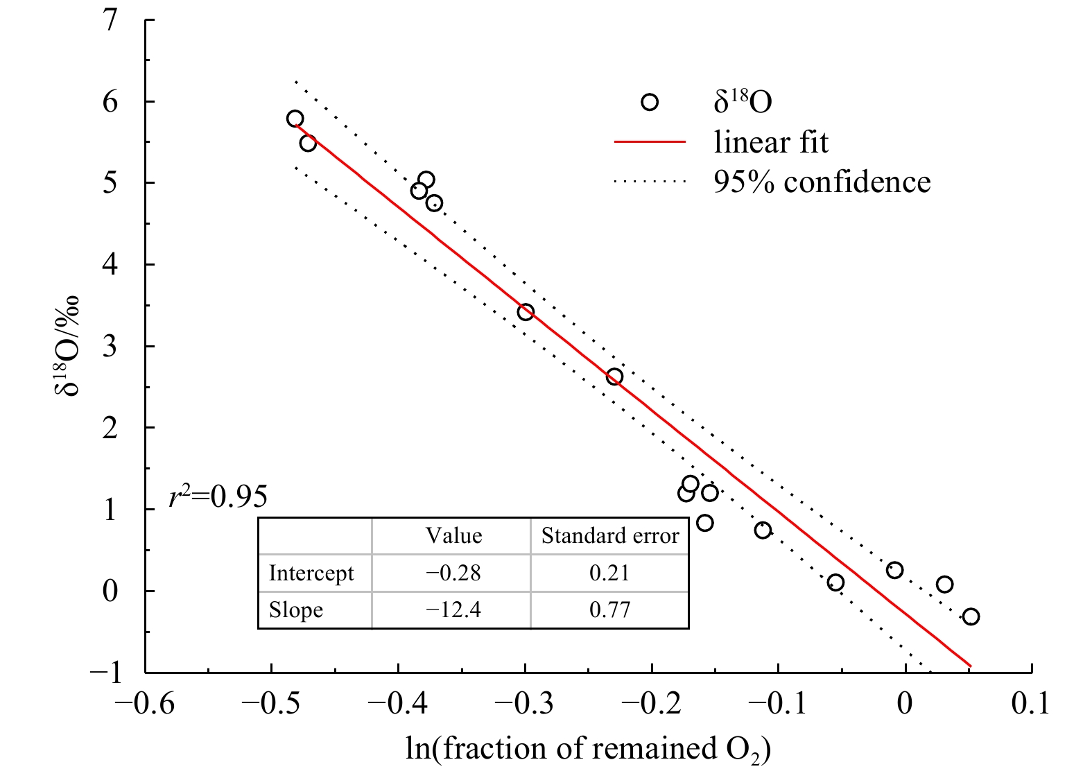
A3.  δ¹⁸O plotted against [O₂] (as ln(fraction of remained O₂)) in this study for both spring and autumn samples beneath the mixed layer.

DownLoad: Full-Size Img PowerPoint

A4.  Nutrients plotted against O₂ properties in the depths where oxygen is depleted (i.e., ([O₂]/[O₂]_eq)_bio < 1). AOV, apparent oxygen utilization.

DownLoad: Full-Size Img PowerPoint