Oyster reefs and their spatial patterns are deemed to change the local hydrodynamic condition and exert profound impacts on the grain size, concentration and transportation of suspended sediments. Meanwhile, high suspended sediment concentration often results in excess mortality among oysters. Oyster reefs are rare and vital ecosystem in Liyashan national marine park, Jiangsu Coast, China. However, urgent conservation efforts should be made on account of the drastic reduction in reef areas. To investigate the sediment dynamics and the geomorphology, two tripod observation systems were deployed and UAV aerial surveys with elevation measurement using Real Time Kinematic (RTK) were also carried out. High mud content (60%) was found in the bed sediment at the reef ridge, causing much lower drag coefficient than other recorded values of living oyster reefs, indicating the death of oysters and the degradation of reefs in Liyashan. Ridgelines of the string reefs at 45° to the current direction and high suspended sediment concentration in the water body (50–370 mg/L) that exceeds the threshold (200 mg/L), which would affect nutrient uptake efficiency and further result in gill saturation, decrease of clearance rate and associated deposition, were probably crucial causes of the death of oysters. The findings are useful for restoring natural oyster reefs and designing artificial reefs for nature-based coastal defense.
Oyster reefs, widely growing in temporal estuaries and littoral areas, refer to large colonial communities that formed by oysters clustering on hard, submerged substrate and propagating by larvae settling on the shells of older or nonliving oysters (Coen and Luckenbach, 2000). Besides supplying edible oysters, oyster reefs also function as the ecosystem engineers that purify waters, provide habitats, stabilize shorelines, fix carbon and couple energy (Chambers et al., 2018; Cressman et al., 2003; Piazza et al., 2005; Quan et al., 2009; Scyphers et al., 2011). Particularly, with increasing risks of storm surge hazards associated with global warming and sea level rise (Bhatia et al., 2018; Slott et al., 2006), the standard of coastal denfence set forth in the past will possibly fail to work in the future and cause security issues (Vousdoukas et al., 2018). Therefore, it appears to be of essence to ensure the restoration of natural oyster reefs and the construction of artificial ones, which manage to attenuate wave energy and thus play a critical role in green coastal engineering (Baine, 2001; Couce et al., 2019; Morris et al., 2019).
However, since 1930s, oyster populations and reef areas underwent a rapid decline due to overfishing, disease and environmental pollution, and hence led to severe ecological and environmental issues in the coastal ecosystems, such as outbreaks of red tides, reduction of fishery resources and degradation of coastal zone (Beck et al., 2011; Brumbaugh and Coen, 2009; Jackson et al., 2001). Human activities will reorganize the spatial distributions of hydrodynamics and suspended sediments, therefore disturb the equilibrium state reached under natural processes and induce subsequent response on oyster reefs, which need to be launched further.
Liyashan National Marine Park, located in Dongzaogang town of Haimen City in the Jiangsu Coast, China, is a rare habitat for living oyster reefs that plays significant roles in biological resources conservation and marine environment protection. Here, the evolution of the oyster reef may have had a history of more than 1 000 years (Chen and Gao, 2010). However, it was just a shadow of its former self as patches of reefs were found buried by sediments, with the decrease of reef areas and the death of living oysters. It follows that expeditious sediment deposition is probably the main reason for the degradation or loss of natural oyster reefs (Quan et al., 2012). Thus, oyster reefs in Liyashan provide a paradigm for studying the mechanisms of oyster reef degradation.
Sedimentary dynamics profoundly affect the diffusion and migration of suspended sediments and pollutants in the shallow sea and estuaries, as well as the evolution and the stability of seabed landforms. The deployment of tripod systems is an effective method for accurate observation in the bottom boundary layer (Cacchione et al., 2006). Thus, to shed light on the effect of human activities on oyster reef habitats and the survival of oysters, observations and researches on sediment dynamics are required (Colden et al., 2016). Besides, with considerable improvements in the techniques of unmanned aerial vehicles and the availability of UAV system, UAV surveys have been widely carried out to observe and quantify the coastal relief (Turner et al., 2016; Cunliffe et al., 2019).
This research comprises two sections. The first part illustrates the geomorphological characteristics of oyster reefs in Liyashan based on Real Time Kinematic (RTK) elevation measurement and UAV aerial surveys, while the second part details and analyzes the sediment dynamic processes using two tripod systems for the observation of hydrodynamics and suspended sediment concentration. The objectives of this paper are thus to: (1) use the resulting UAV imagery to describe the spatial distribution of oyster reefs in the study area and discuss their causes; (2) assess the effects of oyster reefs on hydrodynamics; (3) analyze the causes of oyster reef degradation. The results obtained in the research can provide a basis for the restoration of natural oyster reefs and the construction of artificial reefs.
2.
Study area
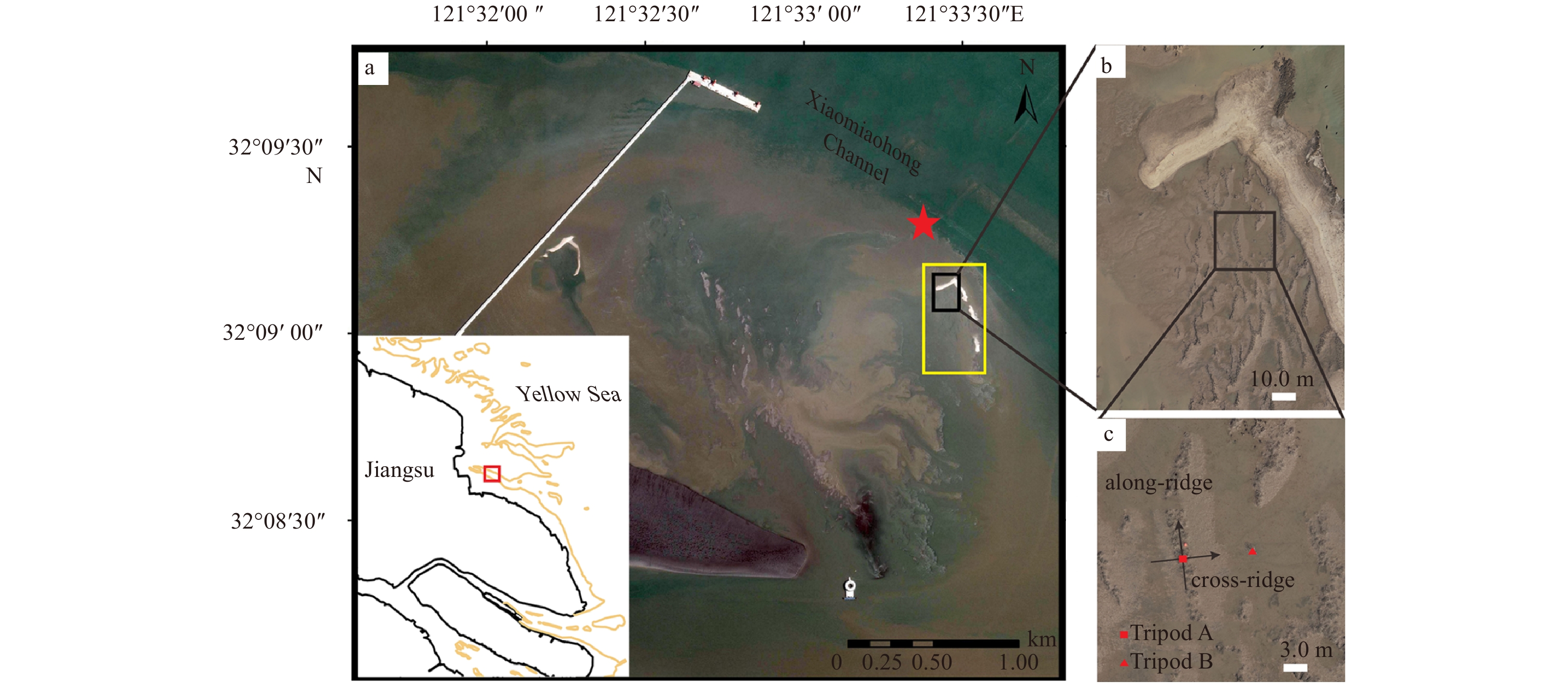
Oyster reefs in the Liyashan national marine park, Haimen, Jiangsu, China, are located on the south side of the western section of Xiaomiaohong Channel (Fig. 1), a large-scale tidal channel that situates in the southern flank of submarine radial sand ridges (Zhang, 2004). The study site herein has a range of scales of oyster reefs, which show an uneven spatial distribution and cover a total area up to approximately 3.56 km2 (Zhang et al., 2007). In spring tides, the submergence duration of oyster reefs occupies 50%–70% of the associated tidal cycle and in neap tides, the inundation period lasts 1–2 d (Quan et al., 2016). The reef-building oysters here are mostly Crassostrea ariakensis and C. gigas, while the living oysters clustering on surface are Ostrea plicatula Gmelin and Crassostrea sikamea (Quan et al., 2012; Zhang, 2004). The field site is characterized by irregular semidiurnal tides as well as large tidal ranges (~2.5 m during the neap tides and ~6 m during the spring tides). As moderate waves dominate in the area, with an annual average significant wave height of 0.3 m, wave action within the research field is considered to be limited (Ren, 1986).
Figure
1.
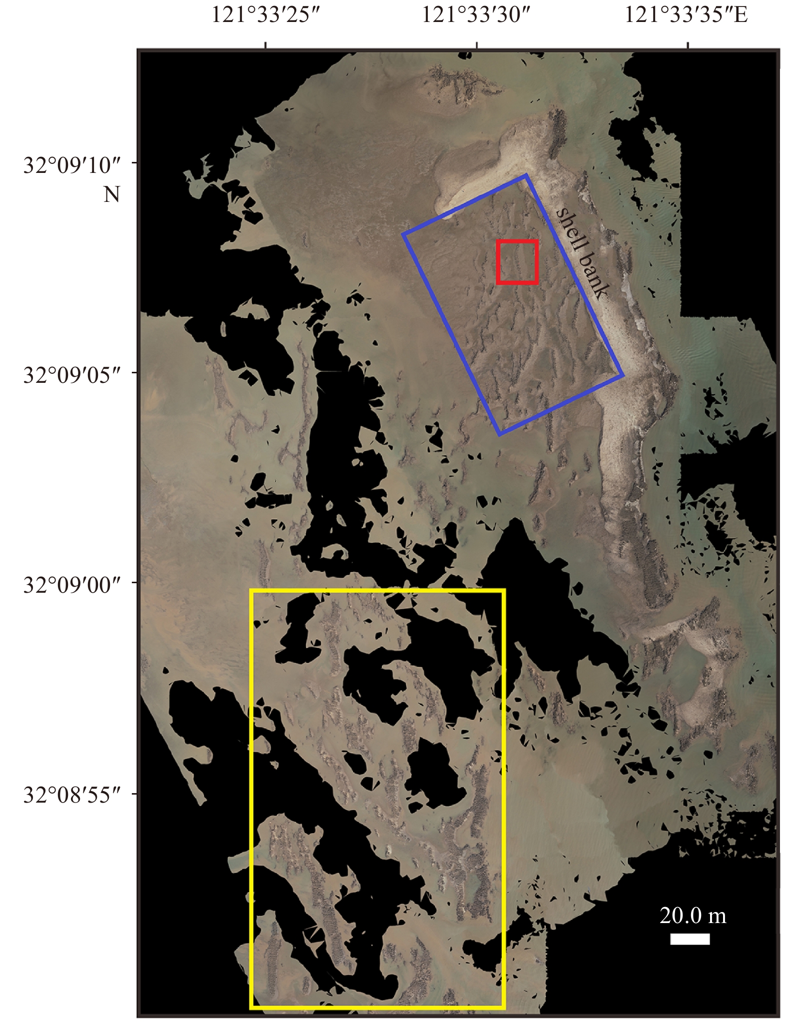
Maps of the study area. a. Location of the Liyanshan oyster reefs in the Jiangsu Coast, China. The yellow frame signifies the area for UAV photography while the red solid denotes the tidal gauge station. b. The target reef behind the shell bank. c. The deployment scheme of two tripod observation systems. The red solid square and triangle denote the Tripod A and Tripod B, respectively. The positive along-ridge and cross-ridge directions are also defined in c.
3.1.1
UAV aerial surveys and RTK elevation measurement
Unmanned aerial vehicles (UAVs) were applied to capture repeated aerial imageries to obtain the spatial pattern of the oyster reefs in Liyashan. The aerial survey was carried out during low tides from 31 October to 2 November using DJI phantom-4-RTK, a UAV type integrated an RTK module that contributes to provide real-time, centimeter-level differential positioning data for enhanced absolute accuracy on image metadata. To cover areas of dense oyster assemblages in the north of the research field, flights were flown at 120 m altitude with 2D photogrammetry mode and three routes were completed on a specific pattern planned by the built-in APP of the remote controller. Due to the broad area of water in the research field, an 80% lateral and longitudinal overlap of images was arranged for creating orthomosaics as previous trials demonstrated (Javernick et al., 2014; Dietrich, 2016). Besides, nine ground control points (GCPs) were employed by a Hi-Target V60 GPS RTK for geolocation accuracy and adopted CGCS 2000 geodetic coordinate in UAV to match the points set above. Positions and elevations of the tripods were also measured by the GPS RTK, alongside the collection of surface sediment in vicinity of the bed at the observation station.
3.1.2
Tripod observation systems
Hydrodynamics observations were carried out in Liyashan oyster reefs between 31 October 2019 and 2 November 2019, which covers around four tidal cycles. Two tripod observation systems were deployed at the reef crest and reef front, namely Tripod A (abbr. TA) and Tripod B (abbr. TB), respectively (Fig. 2). To continuously measure flow motion, suspended sediment concentration and water depth, two acoustic doppler velocimetries (ADV), an optical back scattering (OBS) and two RBR Turbidimeters were installed on each tripod. Specific information of the instrumentation and the sampling scheme are provided in Table 1. Unfortunately, the ADV installed at 0.3 m above sea bed on TA malfunctioned and thereby was not listed. Water samples with suspended sediments were collected near the tripod stations.
Figure
2.
Tripod observation systems A and B at the reef crest and reef front, respectively.
The aerial drone modeling software chosen was Context Capture Smart3D. After adding photos acquired in the field and checking the integrity of the aerial photographs, imported GCPs were marked in matching photograms for block adjustments (Chiabrando et al., 2015) and subsequently aerial triangulation was performed to determine elements of exterior orientation of imageries through the application of the scale-invariant feature transform (SIFT) algorithm (Lowe, 2004). To ensure accurate digitization of a georeferenced image, mapping details were checked, be they the obvious occlusion of feature points or non-negligible horizontal and vertical errors deviated from the GCPs. Confirming the availability of the aerial triangulation achieved above, reconstruction of the 3D mesh model was initially carried out by extracting a detailed three-dimensional point cloud for precision improvement of the following mapping (Castellazzi et al., 2015). The 3D mesh model was then applied to build the orthomosaic and the digital surface models (DSM) and both datasets were able to be exported in Geotiff format. To quantify reef areas, individual oyster reef from the orthomosaics was manually outlined in ArcMap and vectorized to generate polygon feature classes with measurable values of area (m2). UAV-derived elevation values from DSM were also extracted and then compared with GCPs for accuracy evaluations of the DSM.
3.2.2
Current and shear stress
Current velocities from the ADV were averaged over burst, and the velocities were rotated into along-ridge and cross-ridge components, with the positive along-ridge direction being 5.5° anti-clockwise from the north (Fig. 1c).
Reynolds stress method was adopted for estimation of the bed shear stress in shallow water environment (Kim et al., 2000). Thus, the instantaneous current velocity $ u $ was decomposed into a time averaged component $ \overline {u} $ and a turbulence fluctuation component $ {u}' $: $ u=\overline {u}+{u}' $, with $ v $ and $ w $ in the same way. Based on the high-frequency fluctuation components, the eastward and northward shear stresses were calculated as follows and decomposed into along-ridge and cross-ridge parts:
where ${\tau }_{{x}}$, ${\tau }_{{y}}$ represent the eastward, northward shear stresses, respectively and ρ=1 020 kg/m3 is the water density according to the salinity and temperature measured by the OBSs in the field.
3.2.3
Sediment
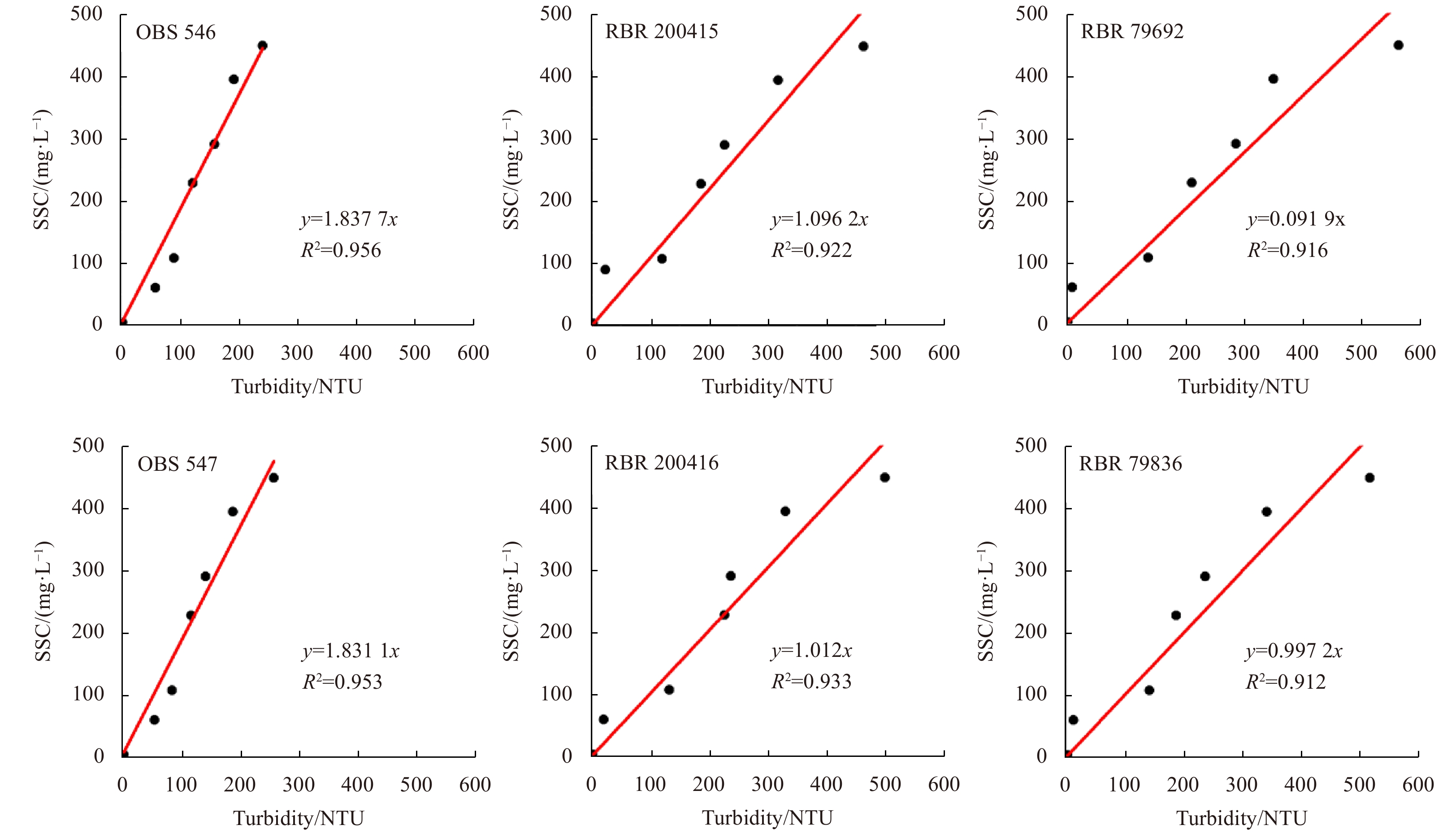
The water samples were vacuum filtered onto preweighed membrane filters, dried (40°C for 48 h) and weighed in the laboratory to calculate suspended sediment concentration (SSC). Considering the relatively low SSC values in this region, the calibrations of the OBS and RBR signals were then achieved by linear regression relating turbidity data (NTU) to SSC (Kineke and Sternberg, 1992; Downing, 2006). The results are shown in Fig. 3.
Figure
3.
Calibration results of the optical back scattering (OBS) and RBR turbidimeters. SSC: suspended sediment concentration.
After pretreatments, suspended and surface sediment samples collected were carried out for laboratory particle-size analysis on the laser diffraction method, performed with a Mastersize 2000 granulometer and relevant dispersion elements manufactured by Malvern Instruments Ltd (Storti and Balsamo, 2010). The average grain diameter as well as sand (62.5–2 000 μm), silt (<4–62.5 μm), and clay fractions (<4 μm), alongside the sorting coefficient and skewness of the samples were then calculated based on the moment method (Blott and Pye, 2001).
4.
Results
4.1
Spatial patterns of oyster reefs in northeastern Liyashan
The generated orthophoto provides useful data over the whole extent of the mapped area, clearly delineating individual reef features as well as displaying spatial patterns of oyster reefs in northeastern Liyashan. Reefs mainly aggregate in the northeastern and southwestern parts of the map, exhibiting uneven distributions (Fig. 4). However, few living oysters were seen on the reefs during the in situ investigation.
Figure
4.
Spatial patterns of the oyster reefs in the northeastern Liyashan. The red frame is the area in Fig. 1c while the blue and yellow frames signify the areas of dense aggregation of fringe reefs and patch reefs (see Fig. 8), respectively; the black patches denote waters where lacks characteristic points for imagery reconstruction.
A shell bank is found in the northeastern of the mapped area (Fig. 4), on which oysters sparsely cover on the seaward side and relatively densely cluster in the southern portion. String reefs aggregate behind the shell bank (blue frame in Fig. 4), with increasing sizes and densities from north to south. Inspection of the orthomosaics shows that string reefs have typical lengths of 10–20 m along ridge and widths of 2–4 m across ridge while the intervals between adjacent reefs range from 5 m to 10 m. The minimum, maximum and average values of the derived reef areas behind the bank are 1.8 m2, 78.7 m2 and 46.2 m2, respectively.
String reefs found in the southwest of the mapped area (yellow frame in Fig. 4) exhibit larger sizes and densities than those closely behind the shell bank. Patch reefs sparsely scatter among the southwestern string reefs, showing smaller reef areas. Investigation of the orthomosaics shows that string reefs in this area have typical lengths of 30–60 m along ridge and widths of 5–10 m across ridge while the intervals between adjacent reefs range from 10 m to 20 m. The minimum, maximum and average values of the derived reef areas in the southwest are 0.5 m2, 313.9 m2 and 105.2 m2, respectively.
Tripod observation systems are situated in the red frame in Fig. 4 and TA is at the center of the ridgeline of the oyster reef (detailed in Fig. 1c), which has a ridge length of around 18.3 m and a width of 2.8 m. According to the elevation difference between TA and TB measured by RTK, the height of the reef crest is derived to be 0.34 m. Water level time series recorded in 2016 from the tidal gauges in the research region was also obtained to combine the effect of the elevation and tidal ranges. Calculation shows that the oyster reefs in the study area are 0.31 m below the mean sea level, with an inundation ratio of 0.76 (Bockelmann et al., 2002; Mudd et al., 2009).
4.2
Hydrodynamics and sediment transport
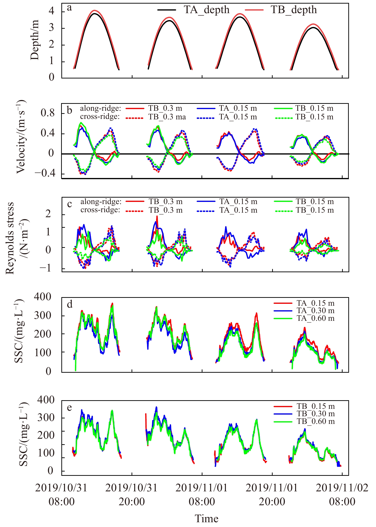
Time series observations were carried out during spring tides, covering four tidal cycles. Results include water depths, along-ridge, cross-ridge velocities and shear stresses at 0.15 m, 0.3 m above sea bed, SSC at 0.15 m, 0.3 m, 0.6 m above sea bed at the reef crest and the reef front (Fig. 5). Note that observation series from the ADV installed at 0.15 m above sea bed at the reef front were erroneous during the third tidal cycle, thus relevant datasets were not delineated in Fig. 5.
Figure
5.
Observational time series of water depth (a), along-, cross-ridge velocity (b), shear stress (c), and suspended sediment concentration (SSC) (d, e) at different layers at the reef crest (named as TA for convenience) and reef front (TB). All the values are above sea bed.
In situ observations manifest typical hydrodynamics conditions with the dominant semidiurnal tide. During the measurement period, the maximum water depth decreased gradually, alongside increasing inundation durations of the reef (Fig. 5a). Maximum water depths in the first two tidal cycles were 3.72 m, 3.30 m while in the last two cycles the values turned to 3.52 m, 2.89 m, respectively.
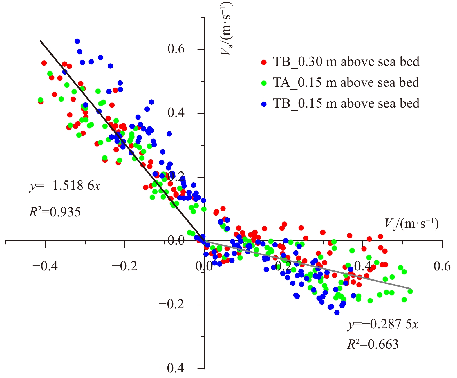
During the observations, the average current velocities calculated at the reef front (0.213 m/s) were slightly larger than those at the reef crest (0.197 m/s). The tidal currents were predominantly characterized by rectilinear flow, alongside somewhat rotary features (Fig. 6). To reflect relationships between the flood/ebb direction and the ridgeline of the reef, the original geographic coordinate was rotated by 5.5° (anti-clockwise) from the north in a local horizontal plane to match the positive along-ridge direction, which was presumed to be 0°. Results showed that the flood direction ranged from 290° to 329°, with an average value of 303°, while the ebb direction varied from 85° to 135°, with an average of 106° (Fig. 6). During the flood periods, the average along-ridge velocities were larger than the cross-ridge ones measured at the same elevation above sea bed of the same tripod, while conditions were on the contrary during the ebb. The aforementioned velocity differences turn to be more obvious over the high tide periods (Fig. 5b). Averagely, the ridge of the string reef was approximately 45° deviated from the flood/ebb direction.
Figure
6.
Velocities near the bed at both the reef crest (TA) and the reef front (TB) (Va, and Vc represent along-ridge and cross-ridge components respectively; straight lines are results of regression analysis and slopes of the black and grey lines denote the average directions of the flood and the ebb, respectively).
During the observations, the average shear stresses calculated at 0.15 m above sea bed at the reef crest (0.64 N/m2) were larger than at 0.15 m above sea bed at the reef front (0.37 N/m2). However, for the derived average shear stresses at the reef front, the smaller values occurred at 0.3 m above sea bed (0.37 N/m2) rather than at 0.15 m above sea bed (0.55 N/m2). During the flood periods, the average along-ridge shear stresses were larger than the cross-ridge ones measured at the same elevation above sea bed of the same tripod, while conditions were on the contrary during the ebb (Fig. 5c). However, for the shear stresses in an identical direction at 0.15 m above sea bed at different tripods, both of the along-ridge and cross-ridge components at the crest (TA) were larger than at the reef front (TB) during flood and ebb periods, which differed from the velocities.
Vertical gradients of suspended sediment concentrations from 0.15 m above sea bed to 0.6 m above sea bed were limited at the reef crest and the front, indicating a relatively uniform SSC layer (Figs 5d and e). Over the observation period, SSCs at 0.15 m, 0.3 m, 0.6 m above sea bed at the reef crest lie in the ranges of, respectively, 52–370 mg/L, 22–333 mg/L, 11–357 mg/L. While at the reef front, the ranges of SSCs were respectively 24–342 mg/L, 24–362 mg/L, 49–343 mg/L at 0.15 m, 0.3 m, 0.6 m above sea bed. Suspended sediment concentrations in the bottom boundary layer varied significantly with tide-induced variances in the flow. The peaks in SSC (>300 mg/L) occurred after the maximum flood/ebb velocities, yet longer peak duration appeared during the flood tides. The SSC then decreased to <100 mg/L due to the settling during slack water before the reversal of the tidal current, corresponding to relatively low velocities and shear stresses and indicating weak resuspension. The averaged suspended sediment concentrations at TA and TB were respectively 192 mg/L and 190 mg/L over the flood periods, both outnumbering values during the ebbs (158 mg/L at TA, 149 mg/L at TB). The maximum SSCs during the flood phase were slightly lower than that during ebbs at the high high tides (the first and the third tidal cycles), while a different story could be told at the low high tides (the second and the fourth tidal cycles) when maximum SSCs were lower during the ebb phase.
4.3
Sediments characteristics
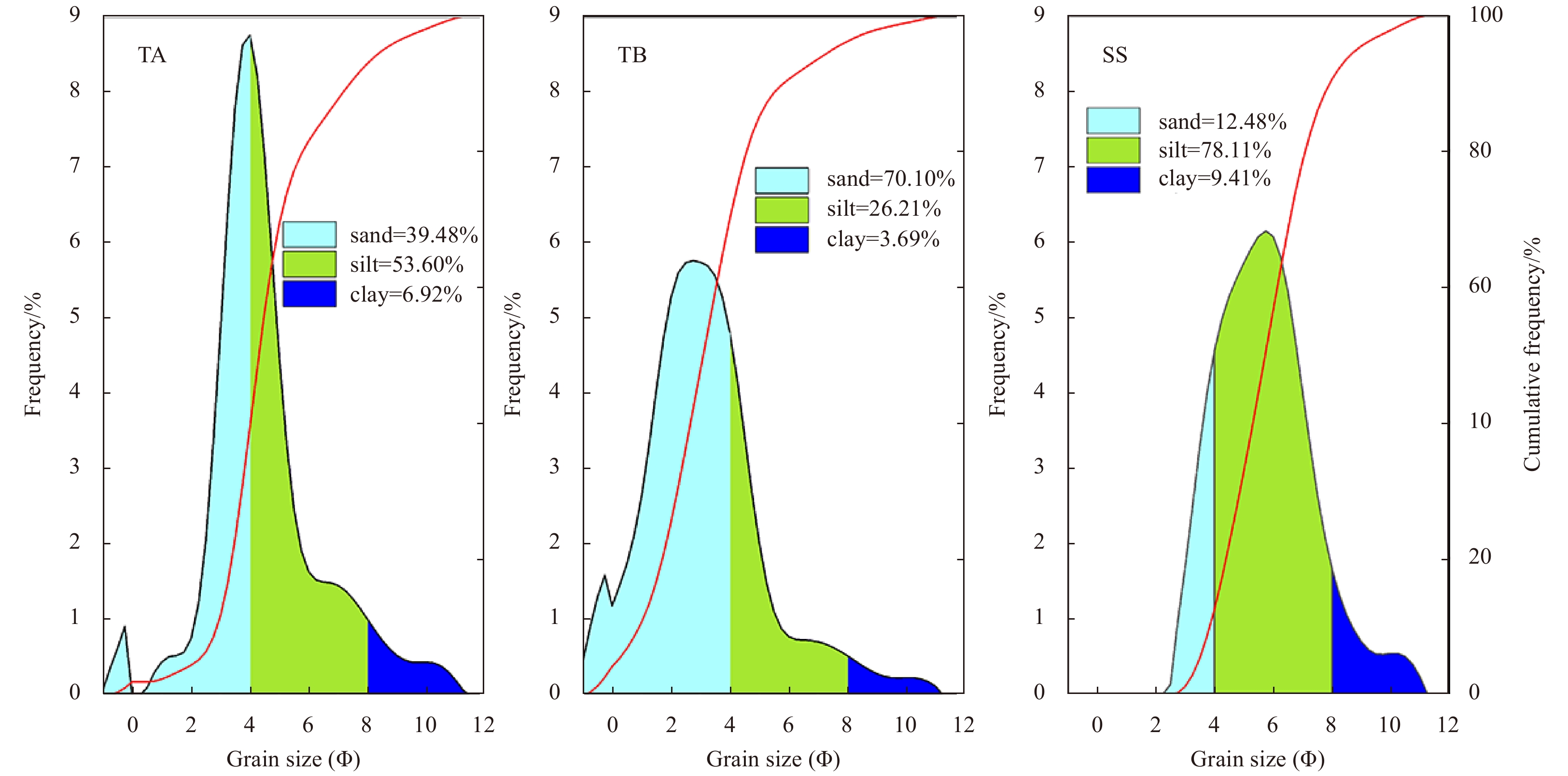
Frequency curves of the suspended and bottom sediment samples collected were shown in Fig. 7, exhibiting a unimodal grain-size distribution with positive skewness and poor sorting. For the surficial bed sediments sampled near TA with the mean grain size of 4.52 Φ, the sand, silt, clay percentages were 39.48%, 53.60%, 6.92%, respectively. The sand content (70.10%) significantly increased in samples collected at TB, with silt and clay percentages down to 26.21% and 3.69%, accounting for the larger mean (3.59 Φ) grain sizes at the reef front. The frequency curve of the suspended sediment sample spanned a narrow range of particle sizes, manifesting the pattern towards finer feature. The mean grain size was 5.72 Φ, while the sand, silt, clay percentages were 12.48%, 78.11%, 9.41%, respectively.
Figure
7.
Grain size and cumulative frequency distributions (the red curves) of the surficial bed sediments at the reef crest (TA) and reef front (TB) and the suspended sediments (SS).
Oyster reefs were found to aggregate behind the shell bank in the northeastern Liyashan and formed recognizable string reef morphologies. String reefs tend to be oriented perpendicular to the tidal currents after trade-offs were entailed between hydrodynamics and reef growth (Grave, 1904; Colden et al., 2016). However, investigation of hydrodynamics in the research region showed the ridgeline of the string reef was approximately at an angle of 45° to the current direction, deviating from the equilibrium state reached under natural conditions. The deviation was presumed to be caused by the reclamation of tidal flats, which contribute to the changes in current direction and velocity (Zhang et al., 2013) and further exert repercussions on the survivability of oysters by decreasing the efficiencies of nutrient uptake and metabolic waste removal (Colden et al., 2016).
Patch reefs sparsely scatter in the southwestern surveyed region, with irregular shapes and relatively smaller areas compared with the adjacent string reefs (Fig. 8). The studies of Grave (1904) and Smith et al. (2003) suggest that patch reefs may be the final stage of evolution of string reefs, which accounts for their small areas and ephemeral existence as well as the unstable nature.
Figure
8.
Spatial distribution of oyster reefs in the southwestern surveyed area (the mapped area corresponds to the yellow frame in Fig. 4 and yellow frames here denote positions of some patch reefs).
Bottom roughness tends to alter the magnitude and structure of turbulence within the bottom boundary layer (Trowbridge and Lentz, 2018), and further exerts impacts on the local and even the large-scale flow as well as the sediment transport, which thus lead to the erosion and deposition processes (Wang et al., 2016). The boundary layer flows also act on the transport of oyster larvae and therefore affect the oyster growth and reef evolution (Dame, 2011).
The drag coefficient was used to quantify the bed roughness and it was computed using the equation:
where $ {\tau }_{0} $ was the bed shear stress, ρ=1 020 kg/m3 was the water density and $ {V}_{0.15\;{\rm m}} $ the burst-averaged velocity at 0.15 m above sea bed and thus $ {C}_{\mathrm{d}0.15\;\mathrm{m}} $ represented the drag coefficient at 0.15 m above sea bed. Results at the reef crest and the reef front are shown in Fig. 9.
Figure
9.
Scatterplot depicting the bed shear stress as a function of the square of the burst-averaged velocity. The slopes of the linear fitting lines equal to the drag coefficients at 0.15 m above sea bed at the reef crest (TA) and the reef front (TB), respectively.
Reefs surveyed in the research region were found with few living oysters, demonstrating an obvious degradation. The drag coefficient at the reef crest is equal to 0.004 3, which is of the same order of the value calculated at the reef front (0.002 8). The present drag coefficient at the reef crest can be compared with some reported values elsewhere (Table 2), e.g., those of degraded reefs being 0.003 7 and 0.009 in the Wreck Shoal and Chesapeake Bay, Virginia, USA, respectively (DeAlteris, 1989; Reidenbach et al., 2013; Whitman and Reidenbach, 2012). It is pronouncedly smaller than that for the degraded reefs in the Mosquito Lagoon (0.016) (Kitsikoudis et al., 2020). Cd calculated at the degraded reef crest was much lower than those of the living oyster reefs (0.01–0.03) (Table 2).
Bottom roughness is crucial in determining bed shear stress and is often partitioned into three components, including grain roughness, sediment saltation roughness and bedform roughness (Xu and Wright, 1995). Biogenic roughness also exerts impacts on the total resistance when biological factors like bioturbation cannot be neglected (Nepf, 2012; Shields et al., 2017). In the case where large bottom roughness of oyster reefs impose substantial drag forces on the overlying flow, the sediment saltation roughness can be ignored as its little contribution to the bottom friction (Wiberg and Rubin, 1989) and thus the bed roughness was decomposed into grain, biogenic and bedform roughness.
Bedform roughness is originated from two scales, including ridge-trough system and bed surface oyster shell levels. Rhythmic reef morphologies shaped by the consecutive ridge-trough system act as bedform roughness and will produce profound resistance on the overlying flow and hence plays an important role in the bottom friction (Constantinescu et al., 2012; Soulsby, 1997). Inspection of the orthomosaics and in situ observation show that string reefs have typical lengths of 101 m along ridge and widths of 100 m while the intervals between adjacent reefs range from 100−101 m. It should be noted that reefs in Liyashan have typical heights of around 0.5 m while healthy oyster reefs are up to 1 m in height (Lenihan, 1999). van Rijn (2007) and Wang et al. (2016) point out that bed roughness height is proportional to the bedform height, thus, compared to living reefs, bedform roughness of degraded reefs is smaller because of lower reef heights.
Ordered arrangement of bed surface oyster shells is another source of bedform roughness. However, due to the vanishment of the oyster filtration activities on the degraded reefs, fine sediments are inclined to be trapped in oyster shells and fill the interstitial space, which will mask and smooth the original surface and result in the decreases in shell heights and losses of rhythmic morphology on the reefs. Likewise, as van Rijn (2007) and Wang et al. (2016) suggested, degraded reefs will show smaller bedform roughness because of lower surface shell heights.
Momentum input of the exhalent jets of bivalves like oysters can also modify the flow at low velocities condition and thus contribute to the biogenic roughness (O’Riordan et al., 1995; van Duren et al., 2006; Wildish and Kristmanson, 1984). The lack of filtration activities on the degraded reefs thus indicates smaller biogenic roughness. Besides, for reefs in the same region, biogenic and bedform roughness are the majority parts while the grain roughness accounts for a small portion. Therefore, with weaker bedform and biogenic roughness, roughness of the degraded reefs is smaller than that of the living reefs in the same region, manifesting as a smaller Cd.
However, for living or degraded reefs in different areas, the distinctions among the drag coefficients listed are not only related to the degradation degree but also deemed to be associated with the bed sediment characteristics, water depths, reef configurations (e.g., reef height and oyster size) and the calculation method for Cd (DeAlteris, 1989; Kitsikoudis et al., 2020; Lenihan and Peterson, 1998; Rothschild et al., 1994). Quantitative explanation of the relationship between the aforementioned causes and degradation degree of reefs remained enigma and deserves further investigations, for its potential to evaluate the degradation degree of oyster reefs more precisely.
5.3
Relationship between oyster growth and suspended sediment characteristic
Bivalves like oysters feed by filtering nutrients in sediments entrained by the overlying flow on one hand, on the other hand, high suspended sediment concentrations can inflict metabolic stress on oysters and are deemed to cause an increase in mortality, albeit for limited enhancement of oyster growth at low SSCs (Dutertre et al., 2009; Huang et al., 2016; Lenihan, 1999; Wilber and Clarke, 2001). Suedel et al. (2015) holds that high suspended sediment concentrations can abrade gill tissues and exert negative impacts on the nutrient intakes, while Barillé et al. (1997) definitely points out that the particle selection efficiency will decrease and lead to a reduction in organics ingestion when SSC exceed 150 mg/L, and the clearance rate stops once the SSC goes beyond 200 mg/L owing to gill saturation. Thus, an SSC of 200 mg/L was adopted as the upper limit for oyster survival to grossly evaluate the suitability of habitats in Liyashan for oysters.
Living oysters in Liyashan are mainly Ostrea plicatula Gmelin and C. sikamea. The study of Li and Shen (2012) suggests that high suspended sediment concentration will affect the enzyme activity of oyster gills and cause DNA damage, which reduce the physiological performances of oysters. Clay particles in sediments cement hydrophobic contaminants like organic toxicity and heavy metals more easily compared with the water phase. Thus, despite the fact that oysters have the ability to detoxify and purify the harmful substances, long exposure duration in high SSC stress will burden metabolism and elicit mortality (Cruz-Rodríguez and Chu, 2002; Eertman et al., 1995). Besides, sediment deposition caused by high suspended sediment concentrations not only produces adverse effects on oyster spat attachment (Carriker, 1986), but also buries adult oysters and significantly increases the death risks of larvae because the resistance to burial sublethal effects is proportional to the shell length (Dunnington, 1968; Colden and Lipcius, 2015).
The peak SSC of oyster reefs in Liyashan is significantly higher than oyster habitats in America (Table 3). During the observation, the suspended sediment concentration ranged from 50 mg/L to 370 mg/L, while the peak SSC appeared to be lower than 100 mg/L in typical oyster habitats in America, such as Chesapeake Bay, Apalachicola Bay and Great Bay Estuary. The SSC in the study area has experienced a conspicuous increase since 2011, with median value increases from 23 mg/L to 78 mg/L to 210 mg/L in 2011, 2014, 2019, respectively (Fig. 10) (Quan et al., 2012, 2016). It is important to note that the median value derived in the current study exceeds the upper limit adopted above (Barillé et al., 1997; Gernez et al., 2014), hence it is plausible to conclude that high suspended sediment concentration is one of the crucial causes of the reef degradation and death of oysters.
Figure
10.
Ranges of suspended sediment concentration (SSC) in Liyashan in recent years. The black dot and the red line denote the median of the interval and the gill saturation threshold, respectively (Quan et al., 2012, 2016).
Oyster reefs in American coast were generally predominated by coarse sediment, usually with sand content greater than 90%. However, for oyster reefs in Liyashan, the mud content (including silt and clay) reaches up to 60% while the sand percentage is less than 40% (Fig. 7). The difference is attributed to the high SSC in the water column, because suspended sediments herein are mostly composed of mud content (about 88%) and increases in SSC can enhance the likelihood of mud deposition and result in associated grain size change in bed components (Carriker, 1986; Dunnington, 1968). The rapid deposition of mud sediment caused by the high SSC will hinder and outpace the growth of oysters and lead to the reef degradation (Colden and Lipcius, 2015), which is presumed responsible for the elimination of oysters in Liyashan.
6.
Conclusions
(1) String reefs were found to aggregate behind the shell bank in the northeastern mapped area, with an inundation ratio of 0.76 and are 0.31 m below mean sea level. The ridgeline of the string reef was at an angle of 45° to the mean current direction, which deviated from the equilibrium state reached under natural conditions and was probably due to the reclamation of tidal flats. Patch reefs were discovered in the southwestern mapped area and they were likely to be end products of string reefs.
(2) The drag coefficient at the reef crest (0.004 3) was larger than that at the reef front (0.002 8), indicating more remarkable bottom friction on the roughness.
(3) During the observation, the interval median of SSC reached up to 210 mg/L, exceeding the upper limit for oyster survival. High suspended sediment concentration in the water body and high content of mud in the bed sediment (60%), which could result in gill saturation, decrease of clearance rate and associated deposition, were probably crucial causes of the death of oysters.
Acknowledgements
The work was supported by Administration Agency of Liyashan National Marine Park, Haimen, Jiangsu, China. We thank Yu Fang and Zhenxing Zhou from Administration Agency of Liyashan National Marine Park for their help in performing field measurements.
Baine M. 2001. Artificial reefs: a review of their design, application, management and performance. Ocean & Coastal Management, 44(3−4): 241–259
[2]
Barillé L, Lerouxel A, Dutertre M, el al. 2011. Growth of the Pacific oyster (Crassostrea gigas) in a high-turbidity environment: comparison of model simulations based on scope for growth and dynamic energy budgets. Journal of Sea Research, 66(4): 392–402. doi: 10.1016/j.seares.2011.07.004
[3]
Barillé L, Prou J, Héral M, et al. 1997. Effects of high natural seston concentrations on the feeding, selection, and absorption of the oyster Crassostrea gigas (Thunberg). Journal of Experimental Marine Biology and Ecology, 212(2): 149–172. doi: 10.1016/S0022-0981(96)02756-6
[4]
Beck M W, Brumbaugh R D, Airoldi L, et al. 2011. Oyster reefs at risk and recommendations for conservation, restoration, and management. Bioscience, 61(2): 107–116. doi: 10.1525/bio.2011.61.2.5
[5]
Bhatia K, Vecchi G, Murakami H, et al. 2018. Projected response of tropical cyclone intensity and intensification in a global climate model. Journal of Climate, 31(20): 8281–8303. doi: 10.1175/JCLI-D-17-0898.1
[6]
Blott S J, Pye K. 2001. GRADISTAT: a grain size distribution and statistics package for the analysis of unconsolidated sediments. Earth Surface Processes and Landforms, 26(11): 1237–1248. doi: 10.1002/esp.261
[7]
Bockelmann A C, Bakker J P, Neuhaus R, et al. 2002. The relation between vegetation zonation, elevation and inundation frequency in a Wadden Sea salt marsh. Aquatic Botany, 73(3): 211–221. doi: 10.1016/S0304-3770(02)00022-0
[8]
Bricker J D, Monismith S G. 2007. Spectral wave-turbulence decomposition. Journal of Atmospheric and Oceanic Technology, 24(8): 1479–1487. doi: 10.1175/JTECH2066.1
[9]
Brumbaugh R D, Coen L D. 2009. Contemporary approaches for small-scale oyster reef restoration to address substrate Versus recruitment limitation: a review and comments relevant for the Olympia oyster, Ostrea lurida carpenter 1864. Journal of Shellfish Research, 28(1): 147–161. doi: 10.2983/035.028.0105
[10]
Cacchione D A, Sternberg R W, Ogston A S. 2006. Bottom instrumented tripods: history, applications, and impacts. Continental Shelf Research, 26(17−18): 2319–2334. doi: 10.1016/j.csr.2006.07.027
[11]
Carriker M R. 1986. Influence of suspended particles on biology of oyster larvae in estuaries. American Malacological Bulletin, 3: 41–49
[12]
Castellazzi G, D'Altri A M, Bitelli G, et al. 2015. From laser scanning to finite element analysis of complex buildings by using a semi-automatic procedure. Sensors, 15(8): 18360–18380. doi: 10.3390/s150818360
[13]
Chambers L G, Gaspar S A, Pilato C J, et al. 2018. How well do restored intertidal oyster reefs support key biogeochemical properties in a coastal lagoon?. Estuaries and Coasts, 41(3): 784–799. doi: 10.1007/s12237-017-0311-5
[14]
Chen Yunzhen, Gao Shu. 2010. A geometric model for oyster reef evolution off southern Jiangsu coast, China. Oceanologia et Limnologia Sinica (in Chinese), 41(1): 1–11
[15]
Chiabrando F, Donadio E, Rinaudo F. 2015. SfM for orthophoto to generation: a winning approach for cultural heritage knowledge. In: Proceedings of the International Archives of Photogrammetry, Remote Sensing and Spatial Information Sciences. Taipei: ISPRS, 91–98
[16]
Coen L D, Luckenbach M W. 2000. Developing success criteria and goals for evaluating oyster reef restoration: ecological function or resource exploitation?. Ecological Engineering, 15(3−4): 323–343. doi: 10.1016/S0925-8574(00)00084-7
[17]
Colden A M, Fall K A, Cartwright G M, et al. 2016. Sediment suspension and deposition across restored oyster reefs of varying orientation to flow: implications for restoration. Estuaries and Coasts, 39(5): 1435–1448. doi: 10.1007/s12237-016-0096-y
[18]
Colden A M, Lipcius R N. 2015. Lethal and sublethal effects of sediment burial on the eastern oyster Crassostrea virginica. Marine Ecology Progress Series, 527: 105–117. doi: 10.3354/meps11244
[19]
Constantinescu G, Miyawaki S, Liao Qian. 2012. Flow and turbulence structure past a cluster of freshwater mussels. Journal of Hydraulic Engineering, 139(4): 347–358
[20]
Couce L M C, Guerreiro M J R, Formoso J A F, et al. 2019. Green artificial reef PROARR: repopulation of coastal ecosystems and waste recycler of the maritime industries. In: Proceedings of the 25th Pan-American Conference of Naval Engineering. Cham, Switzerland: Springer, 363–373
[21]
Cressman K A, Posey M H, Mallin M A, et al. 2003. Effects of oyster reefs on water quality in a tidal creek estuary. Journal of Shellfish Research, 22(3): 753–762
[22]
Cruz-Rodríguez L A, Chu F L E. 2002. Heat-shock protein (HSP70) response in the eastern oyster, Crassostrea virginica, exposed to PAHs sorbed to suspended artificial clay particles and to suspended field contaminated sediments. Aquatic Toxicology, 60(3−4): 157–168. doi: 10.1016/S0166-445X(02)00008-5
[23]
Cunliffe A M, Tanski G, Radosavljevic B, et al. 2019. Rapid retreat of permafrost coastline observed with aerial drone photogrammetry. The Cryosphere, 13(5): 1513–1528. doi: 10.5194/tc-13-1513-2019
[24]
Dame R F. 2011. Ecology of Marine Bivalves: An Ecosystem Approach. 2nd ed. Boca Raton, FL, USA: CRC Press
[25]
DeAlteris J T. 1989. The role of bottom current and estuarine geomorphology on the sedimentation processes and productivity of wreck shoal, an oyster reef of the James River, Virginia. In: Neilson B J, Kuo A, Brubaker J, eds. Estuarine Circulation. Clifton, NJ, USA: Humana Press, 279–307
[26]
Dietrich J T. 2016. Riverscape mapping with helicopter-based Structure-from-Motion photogrammetry. Geomorphology, 252: 144–157. doi: 10.1016/j.geomorph.2015.05.008
[27]
Downing J. 2006. Twenty-five years with OBS sensors: the good, the bad, and the ugly. Continental Shelf Research, 26(17−18): 2299–2318. doi: 10.1016/j.csr.2006.07.018
[28]
Dunnington E A Jr. 1968. Survival time of oysters after burial at various temperatures. Proceedings of the National Shellfisheries Association, 58: 101–103
[29]
Dutertre M, Beninger P G, Barillé L, et al. 2009. Temperature and seston quantity and quality effects on field reproduction of farmed oysters, Crassostrea gigas, in Bourgneuf Bay, France. Aquatic Living Resources, 22(3): 319–329. doi: 10.1051/alr/2009042
[30]
Eertman R H M, Groenink C L F M G, Sandee B, et al. 1995. Response of the blue mussel Mytilus edulis L. following exposure to PAHs or contaminated sediment. Marine Environmental Research, 39(1−4): 169–173. doi: 10.1016/0141-1136(94)00022-H
[31]
Gernez P, Barillé L, Lerouxel A, et al. 2014. Remote sensing of suspended particulate matter in turbid oyster-farming ecosystems. Journal of Geophysical Research: Oceans, 119(10): 7277–7294. doi: 10.1002/2014JC010055
[32]
Goring D G, Nikora V I. 2002. Despiking acoustic Doppler velocimeter data. Journal of hydraulic engineering, 128(1): 117–126. doi: 10.1061/(ASCE)0733-9429(2002)128:1(117)
[33]
Grave C. 1904. Investigations for the promotion of the oyster industry of North Carolina (Vol. 556). University of Michigan Library, 67−101
[34]
Huang Wenrui, Hagen S C, Wang Dingbao, et al. 2016. Suspended sediment projections in Apalachicola Bay in response to altered river flow and sediment loads under climate change and sea level rise. Earth’s Future, 4(10): 428–439. doi: 10.1002/2016EF000384
[35]
Jackson J B C, Kirby M X, Berger W H, et al. 2001. Historical overfishing and the recent collapse of coastal ecosystems. Science, 293(5530): 629–637. doi: 10.1126/science.1059199
[36]
Javernick L, Brasington J, Caruso B. 2014. Modeling the topography of shallow braided rivers using Structure-from-Motion photogrammetry. Geomorphology, 213: 166–182. doi: 10.1016/j.geomorph.2014.01.006
[37]
Kennedy V S, Sanford L P. 1999. The morphology and physical oceanography of unexploited oyster reefs in North America. In: Luckenbach M W, Mann R, Wesson J A, eds. Oyster Reef Habitat Restoration: A Synopsis and Synthesis of Approaches. Gloucester Point, VA, USA: VIMS Press, 25–46
[38]
Kim S C, Friedrichs C T, Maa J P Y, et al. 2000. Estimating bottom stress in tidal boundary layer from acoustic Doppler velocimeter data. Journal of Hydraulic Engineering, 126(6): 399–406. doi: 10.1061/(ASCE)0733-9429(2000)126:6(399)
[39]
Kineke G C, Sternberg R W. 1992. Measurements of high concentration suspended sediments using the optical backscatterance sensor. Marine Geology, 108(3−4): 253–258. doi: 10.1016/0025-3227(92)90199-R
[40]
Kitsikoudis V, Kibler K M, Walters L J. 2020. In-situ measurements of turbulent flow over intertidal natural and degraded oyster reefs in an estuarine lagoon. Ecological Engineering, 143: 105688. doi: 10.1016/j.ecoleng.2019.105688
[41]
Lenihan H S. 1999. Physical-biological coupling on oyster reefs: how habitat structure influences individual performance. Ecological Monographs, 69(3): 251–275
[42]
Lenihan H S, Peterson C H. 1998. How habitat degradation through fishery disturbance enhances impacts of hypoxia on oyster reefs. Ecological Applications, 8(1): 128–140. doi: 10.1890/1051-0761(1998)008[0128:HHDTFD]2.0.CO;2
[43]
Li Yun, Shen Anglu. 2012. Damage and recovery in the Kumamoto oyster Crassostrea sikamea stressed by suspended solids. Journal of Fishery Sciences of China (in Chinese), 19(1): 138–144
[44]
Liu Huan, Wu Chaoyu. 2011. Turbulence measurement in estuary and data post-processing. The Ocean Engineering (in Chinese), 29(2): 122–128, 134
[45]
Lowe D G. 2004. Distinctive image features from scale-invariant keypoints. International Journal of Computer Vision, 60(2): 91–110. doi: 10.1023/B:VISI.0000029664.99615.94
[46]
Lu Yuanzheng, Wu Jiaxue, Liu Huan. 2012. An integrated post-processing technique for turbulent flows in estuarine bottom boundary layer. Haiyang Xuebao (in Chinese), 34(5): 39–49
[47]
MacVean L J, Lacy J R. 2014. Interactions between waves, sediment, and turbulence on a shallow estuarine mudflat. Journal of Geophysical Research: Oceans, 119(3): 1534–1553. doi: 10.1002/2013JC009477
[48]
Morris R L, Bilkovic D M, Boswell M K, et al. 2019. The application of oyster reefs in shoreline protection: are we over-engineering for an ecosystem engineer?. Journal of Applied Ecology, 56(7): 1703–1711. doi: 10.1111/1365-2664.13390
[49]
Mudd S M, Howell S M, Morris J T. 2009. Impact of dynamic feedbacks between sedimentation, sea-level rise, and biomass production on near-surface marsh stratigraphy and carbon accumulation. Estuarine, Coastal and Shelf Science, 82(3): 377–389. doi: 10.1016/j.ecss.2009.01.028
[50]
Nepf H M. 2012. Flow and transport in regions with aquatic vegetation. Annual Review of Fluid Mechanics, 44: 123–142. doi: 10.1146/annurev-fluid-120710-101048
[51]
O’Riordan C A, Monismith S G, Koseff J R. 1995. The effect of bivalve excurrent jet dynamics on mass transfer in a benthic boundary layer. Limnology and Oceanography, 40(2): 330–344. doi: 10.4319/lo.1995.40.2.0330
[52]
Piazza B P, Banks P D, La Peyre M K. 2005. The potential for created oyster shell reefs as a sustainable shoreline protection strategy in Louisiana. Restoration Ecology, 13(3): 499–506. doi: 10.1111/j.1526-100X.2005.00062.x
[53]
Quan Weimin, An Chuangguang, Ma Chunyan, et al. 2012. Biodiversity and community structure of benthic macroinvertebrates on the Xiaomiaohong oyster reef in Jiangsu Province, China. Oceanologia et Limnologia Sinica (in Chinese), 43(5): 992–1000
[54]
Quan Weimin, Zhou Weifeng, Ma Chunyan, et al. 2016. Ecological status of a natural intertidal oyster reef in Haimen County, Jiangsu Province. Acta Ecologica Sinica (in Chinese), 36(23): 7749–7757
[55]
Quan Weimin, Zhu Jiangxing, Ni Yong, et al. 2009. Faunal utilization of constructed intertidal oyster (Crassostrea rivularis) reef in the Yangtze River estuary, China. Ecological Engineering, 35(10): 1466–1475. doi: 10.1016/j.ecoleng.2009.06.001
[56]
Reidenbach M A, Berg P, Hume A, et al. 2013. Hydrodynamics of intertidal oyster reefs: the influence of boundary layer flow processes on sediment and oxygen exchange. Limnology and Oceanography: Fluids and Environments, 3(1): 225–239. doi: 10.1215/21573689-2395266
[57]
Ren M E. 1986. Comprehensive Investigation of the Coastal Zone and Tidal Land Resources of Jiangsu Province (in Chinese). Beijing: China Ocean Press, 184–192
[58]
Rothschild B J, Ault J S, Goulletquer P, et al. 1994. Decline of the Chesapeake Bay oyster population: a century of habitat destruction and overfishing. Marine Ecology Progress Series, 111: 29–39. doi: 10.3354/meps111029
[59]
Scyphers S B, Powers S P, Heck Jr K L, et al. 2011. Oyster reefs as natural breakwaters mitigate shoreline loss and facilitate fisheries. PLoS ONE, 6(8): e22396. doi: 10.1371/journal.pone.0022396
[60]
Shields Jr F D, Coulton K G, Nepf H. 2017. Representation of vegetation in two-dimensional hydrodynamic models. Journal of Hydraulic Engineering, 143(8): 02517002. doi: 10.1061/(ASCE)HY.1943-7900.0001320
[61]
Slott J M, Murray A B, Ashton A D, et al. 2006. Coastline responses to changing storm patterns. Geophysical Research Letters, 33(18): L18404
[62]
Smith G F, Roach E B, Bruce D G. 2003. The location, composition, and origin of oyster bars in mesohaline Chesapeake Bay. Estuarine, Coastal and Shelf Science, 56(2): 391–409. doi: 10.1016/S0272-7714(02)00191-9
[63]
Soulsby R L. 1997. Dynamics of Marine Sands: A Manual for Practical Applications. London, UK: Thomas Telford
[64]
Storti F, Balsamo F. 2010. Particle size distributions by laser diffraction: sensitivity of granular matter strength to analytical operating procedures. Solid Earth, 1(1): 25–48. doi: 10.5194/se-1-25-2010
[65]
Styles R. 2015. Flow and turbulence over an oyster reef. Journal of Coastal Research, 31(4): 978–985
[66]
Suedel B C, Clarke J U, Wilkens J, et al. 2015. The effects of a simulated suspended sediment plume on eastern oyster (Crassostrea virginica) survival, growth, and condition. Estuaries and Coasts, 38(2): 578–589. doi: 10.1007/s12237-014-9835-0
[67]
Trowbridge J H, Lentz S J. 2018. The bottom boundary layer. Annual Review of Marine Science, 10: 397–420. doi: 10.1146/annurev-marine-121916-063351
[68]
Turner I L, Harley M D, Drummond C D. 2016. UAVs for coastal surveying. Coastal Engineering, 114: 19–24. doi: 10.1016/j.coastaleng.2016.03.011
[69]
van Duren L A, Herman P M J, Sandee A J J, et al. 2006. Effects of mussel filtering activity on boundary layer structure. Journal of Sea Research, 55(1): 3–14. doi: 10.1016/j.seares.2005.08.001
[70]
van Rijn L C. 2007. Unified view of sediment transport by currents and waves. I: initiation of motion, bed roughness, and bed-load transport. Journal of Hydraulic Engineering, 133(6): 649–667. doi: 10.1061/(ASCE)0733-9429(2007)133:6(649)
[71]
Vousdoukas M I, Mentaschi L, Voukouvalas E, et al. 2018. Climatic and socioeconomic controls of future coastal flood risk in Europe. Nature Climate Change, 8(9): 776–780. doi: 10.1038/s41558-018-0260-4
[72]
Wang Yunwei, Yu Qian, Jiao Jian, et al. 2016. Coupling bedform roughness and sediment grain-size sorting in modelling of tidal inlet incision. Marine Geology, 381: 128–141. doi: 10.1016/j.margeo.2016.09.004
[73]
Whitman E R, Reidenbach M A. 2012. Benthic flow environments affect recruitment of Crassostrea virginica larvae to an intertidal oyster reef. Marine Ecology Progress Series, 463: 177–191. doi: 10.3354/meps09882
[74]
Wiberg P L, Rubin D M. 1989. Bed roughness produced by saltating sediment. Journal of Geophysical Research: Oceans, 94(C4): 5011–5016. doi: 10.1029/JC094iC04p05011
[75]
Wilber D H, Clarke D G. 2001. Biological effects of suspended sediments: a review of suspended sediment impacts on fish and shellfish with relation to dredging activities in estuaries. North American Journal of Fisheries Management, 21(4): 855–875. doi: 10.1577/1548-8675(2001)021<0855:BEOSSA>2.0.CO;2
[76]
Wildish D J, Kristmanson D D. 1984. Importance to mussels of the benthic boundary layer. Canadian Journal of Fisheries and Aquatic Sciences, 41(11): 1618–1625. doi: 10.1139/f84-200
[77]
Xiong Jilian, Wang Xiaohua, Wang Yaping, et al. 2018. Reprint of Mechanisms of maintaining high suspended sediment concentration over tide-dominated offshore shoals in the southern Yellow Sea. Estuarine, Coastal and Shelf Science, 206: 2–13. doi: 10.1016/j.ecss.2018.03.019
[78]
Xu J P, Wright L D. 1995. Tests of bed roughness models using field data from the Middle Atlantic Bight. Continental Shelf Research, 15(11−12): 1409–1434. doi: 10.1016/0278-4343(94)00083-Y
[79]
Zappas J, Moskalski S. 2018. Suspended sediment concentration and sediment flux over a restored oyster reef. In: Proceedings of the Northeastern Section-53rd Annual Meeting-2018. Galloway, Scotland: GSA
[80]
Zhang Renshun. 2004. The geomorphology-sedimentology character of oyster reef in Xiaomiaohong tidal channel, Jiangsu Province. Oceanologia et Limnologia Sinica (in Chinese), 35(1): 1–7
[81]
Zhang Renshun, Wang Yanhong, Zhang Zhenglong, et al. 2007. Geomorphology and evolution of the Xiaomiaohong Oyster reef off Jiangsu coast, China. Oceanologia et Limnologia Sinica (in Chinese), 38(3): 259–265
[82]
Zhang Chi, Zheng Jinhai, Dong Xiaowei, et al. 2013. Morphodynamic response of Xiaomiaohong tidal channel to a coastal reclamation project in Jiangsu Coast, China. Journal of Coastal Research, 1(65): 630–635
Jiaquan Zhuang, Qian Yu, Yidong Guo, et al. Decoding intertidal oyster reef morphology: Insights from UAV photogrammetry and deep learning. Marine Geology, 2025, 480: 107462. doi:10.1016/j.margeo.2024.107462
2.
Qian Yu, Jianjun Jia, Shu Gao. Scientific basis, engineering feasibility and system optimization of green sea dykes for temperate mud coasts: a brief overview. Anthropocene Coasts, 2024, 7(1) doi:10.1007/s44218-024-00052-y
3.
Jiaquan Zhuang, Yunwei Wang, Yidong Guo, et al. High-resolution DEMs reveal multi-scale roughness of oyster reefs via smartphone photogrammetry. Geo-Marine Letters, 2024, 44(4) doi:10.1007/s00367-024-00785-2
4.
Li‐Sha Hu, Yun‐Wei Dong. Multiple genetic sources facilitate the northward range expansion of an intertidal oyster along China's coast. Ecological Applications, 2024, 34(1) doi:10.1002/eap.2764
5.
Bingxian Liu, Zhenqiang Liu, Ya Chen, et al. Potential distribution of Crassostrea sikamea (Amemiya, 1928) along coastal China under global climate change. Global Ecology and Conservation, 2024, 50: e02843. doi:10.1016/j.gecco.2024.e02843
6.
Thomas Dunlop, William Glamore, Stefan Felder. Restoring estuarine ecosystems using nature-based solutions: Towards an integrated eco-engineering design guideline. Science of The Total Environment, 2023, 873: 162362. doi:10.1016/j.scitotenv.2023.162362
7.
V Perricone, M Mutalipassi, A Mele, et al. Nature-based and bioinspired solutions for coastal protection: an overview among key ecosystems and a promising pathway for new functional and sustainable designs. ICES Journal of Marine Science, 2023, 80(5): 1218. doi:10.1093/icesjms/fsad080
8.
Xinmeng Wang, Jihong Zhang, Yi Zhong, et al. GIS-based spatial suitability assessment for pacific oyster Crassostrea gigas reef restoration: A case study of Laizhou Bay, China. Marine Pollution Bulletin, 2023, 186: 114416. doi:10.1016/j.marpolbul.2022.114416
9.
Feng Luo, Zhipeng Chen, Hongbo Wu, et al. Hydrodynamic and sediment dynamic impact of human engineering activity on Liyashan oyster reefs, China. Frontiers in Marine Science, 2022, 9 doi:10.3389/fmars.2022.1051868
Figure 1. Maps of the study area. a. Location of the Liyanshan oyster reefs in the Jiangsu Coast, China. The yellow frame signifies the area for UAV photography while the red solid denotes the tidal gauge station. b. The target reef behind the shell bank. c. The deployment scheme of two tripod observation systems. The red solid square and triangle denote the Tripod A and Tripod B, respectively. The positive along-ridge and cross-ridge directions are also defined in c.
Figure 2. Tripod observation systems A and B at the reef crest and reef front, respectively.
Figure 3. Calibration results of the optical back scattering (OBS) and RBR turbidimeters. SSC: suspended sediment concentration.
Figure 4. Spatial patterns of the oyster reefs in the northeastern Liyashan. The red frame is the area in Fig. 1c while the blue and yellow frames signify the areas of dense aggregation of fringe reefs and patch reefs (see Fig. 8), respectively; the black patches denote waters where lacks characteristic points for imagery reconstruction.
Figure 5. Observational time series of water depth (a), along-, cross-ridge velocity (b), shear stress (c), and suspended sediment concentration (SSC) (d, e) at different layers at the reef crest (named as TA for convenience) and reef front (TB). All the values are above sea bed.
Figure 6. Velocities near the bed at both the reef crest (TA) and the reef front (TB) (Va, and Vc represent along-ridge and cross-ridge components respectively; straight lines are results of regression analysis and slopes of the black and grey lines denote the average directions of the flood and the ebb, respectively).
Figure 7. Grain size and cumulative frequency distributions (the red curves) of the surficial bed sediments at the reef crest (TA) and reef front (TB) and the suspended sediments (SS).
Figure 8. Spatial distribution of oyster reefs in the southwestern surveyed area (the mapped area corresponds to the yellow frame in Fig. 4 and yellow frames here denote positions of some patch reefs).
Figure 9. Scatterplot depicting the bed shear stress as a function of the square of the burst-averaged velocity. The slopes of the linear fitting lines equal to the drag coefficients at 0.15 m above sea bed at the reef crest (TA) and the reef front (TB), respectively.
Figure 10. Ranges of suspended sediment concentration (SSC) in Liyashan in recent years. The black dot and the red line denote the median of the interval and the gill saturation threshold, respectively (Quan et al., 2012, 2016).


 DownLoad:

 DownLoad:


 DownLoad: