Figure
1.
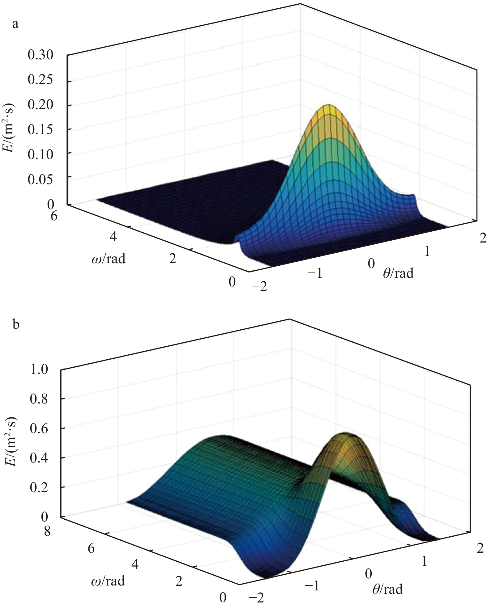
Spectrum distribution of JONSWAP spectrum.
| Citation: | Zhimiao Chang, Fuxing Han, Zhangqing Sun, Zhenghui Gao, Lili Wang. Three-dimensional dynamic sea surface modeling based on ocean wave spectrum[J]. Acta Oceanologica Sinica, 2021, 40(10): 38-48. doi: 10.1007/s13131-021-1871-6

|
In conventional marine seismic data acquisition and processing, researchers always regard sea surface as horizontal boundary (Cecconello et al., 2018). However, because of sea breezes and waves, the sea surface is undulating. This phenomenon causes the ray paths changing during the actual propagation process (Meng et al., 2019). Due to the dynamic feature of sea surface, it cannot be treated exactly the same as that of conventional surface undulation correction, and that results in large errors (Laws and Kragh, 2002; Wang et al., 2007; Qi, 2015). In order to grasp the fluctuation of sea surface and the impact on energy propagation more accurately, it is necessary to conduct in-depth research on dynamic modeling methods of undulating sea surface.
The modeling methods of dynamic sea surface are mainly divided into two categories, physical modeling method and mathematical modeling method.
The physical method bases on Navier-Stokes equations. This method regards fluid as a whole, and by using numerical simulation, calculates the overall force of the fluid, then simulating the undulating sea state (Liu et al., 1998; Wu et al., 2008). Alternatively, it regards the fluid as particles, by using Smooth Particle Hydrodynamics (SPH) algorithm to simulate sea surface at the micro level, and then it is easy to show the movement pattern of water body macroscopically (Monaghan, 2005; Sun and Wang, 2007; Shen et al., 2020).
The mathematical modeling method combines Statistics and Geometry (Phillips, 1958; Fournier and Reeves, 1986; Liu et al., 2006; Li et al., 2006; Qi et al., 2013; Pierson and Moskowitz, 1964). The basic structure of the algorithm is using the empirical equation of ocean wave spectrum obtained by statistics, substituting the equation of geometric shape parameter; after superposition, the similar real undulating sea surface can be obtained. For example, simple harmonic method and Gerstner method. Besides, in recent years, the use of high-order spectrum to simulate the sea surface can effectively simulate freak waves (Dommermuth and Yue, 1987; Zhang et al., 2013), and it has gradually begun to attract researchers’ attention.
Both of these methods have advantages and disadvantages. Although the physical method makes the sea surface conform to the laws of physics, it is not widely used in the real-time simulation of the sea surface due to its extremely long calculation period and complex steady-state process. The major advantage of math method is the fast calculation speed. After combining the wave spectrum parameters, the simulated sea surface fluctuations are realistic.
Considering the advantages and disadvantages of above methods, this paper will start from the mathematical simulation method to study the realization process and the realization effect of the three simulation methods, including simple harmonics, Gerstner wave and wave equation, and compare the three methods in terms of calculation speed and model characteristics. In order to show the differences among the three methods better, the wave spectrum during the calculations are all carried out by JONSWAP spectrum, and the direction distribution function recommended by Stereo Wave Observation Project (SWOP; Cote, 1960) is used to convert the ocean wave spectrum to JONSWAP direction spectrum function. On the basis of three simulation methods, comprehensively considering the advantages and disadvantages of each method, a dynamic boundary condition of the sea surface is proposed. This boundary condition can be applied to the wave equation method to simulate the sea surface, so that it can hardly lose the calculation speed. It shows the state of the sea surface advance more clearly. A simple comparison between the improved wave equation method and the high-order spectrum method for sea surface simulation effects will also be made to show the characteristics of the wave equation method.
In order to meet the development needs of the North Sea, from 1968 to 1970, the United Kingdom, the Netherlands, the United States, Germany and other relevant institutions jointly conducted the “Joint North Sea Wave Project” (JONSWAP). Systematic wave observations were carried out in Denmark and western Germany (Hasselmann, 1973; Hasselmann et al., 1976).
A very systematic observation was made on the 160 km section, and a total of 2 500 spectra were obtained. Under the action of the east wind, the deep-water wind and waves appearing at each station are helpful to study the process of wind and waves growing with the wind. For example, the waves in the Atlantic Ocean propagate from the west to the coast, which is beneficial to the study of the transformation of swells in diving. This is by far the most systematic ocean wave observation work.
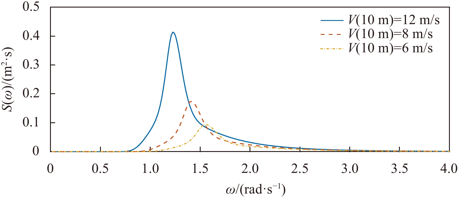
Using these results, through estimation and fitting, the JONSWAP spectrum (Fig. 1) with higher accuracy is obtained. This is a deep-water spectrum, which is not applicable to shallow seas. The specific expression is
| $$\begin{split} {{S}_{\zeta }\left(\omega \right)=}{\frac{\alpha {g}^{2}}{{\omega }^{5}}\exp\left[-1.25{\left(\frac{{\omega }_{p}}{\omega }\right)}^{4}\right]{\gamma }^{\exp\left[\frac{\omega -{\omega }_{p}}{2(\sigma {\omega }_{p}{)}^{2}}\right]}}{,} \end{split} $$ | (1) |
where
| $$ \sigma =\left\{\begin{split}0.07\;\;\omega \leqslant {\omega }_{p}\\ 0.09\;\;\omega > {\omega }_{p}\end{split}\right.. $$ |
Figure 1 shows the energy distribution of the JONSWAP spectrum under different wind speeds. It can be seen from the figure that the higher the wind speed, the more concentrated the energy and the narrower the frequency band.
For marine seismic exploration, due to the fast propagation speed of artificial seismic waves, the maximum range of seismic wave energy coverage is usually above the kilometer level, so the wind range parameters in the JONSWAP spectrum should be appropriately selected larger. The wind range
Since the sea surface is three-dimensional, the two-dimensional wave needs to be converted to the three-dimensional sea surface, and the conversion method adopts the direction spectrum function. When the wind direction is constant, the sea surface in the wind direction should satisfy a certain wave spectrum. In the fan-shape area on left and right of the wind direction, the energy of the waves will attenuate, and the entire energy distribution is no longer in a straight line. The nature of the direction spectrum function is an energy distribution relationship. The JONSWAP direction spectrum can be expressed as:
| $$ {S}_{\rm{JONSWAP}}\left(\omega{,}\theta \right)=S\left(\omega\right)G\left(\omega{,}\theta \right){,} $$ | (2) |
where
| $$ \begin{split} {G\left(\omega{,}\theta \right)=}{\frac{1}{\pi }\left[1+p{\rm{cos}}\left(2\theta \right)+q{\rm{cos}}\left(4\theta \right)\right]{,}\;\theta \leqslant \frac{\pi }{2}{,}} \end{split} $$ | (3) |
where
Figure 2a shows the characteristics of the directional distribution function. It can be seen from Fig. 2a that at the positive wind direction 0, the energy of the waves is the largest, while the energy on both sides gradually attenuates. Figure 2b shows the distribution of the JONSWAP directional spectrum. It has the same pattern as Fig. 2a.

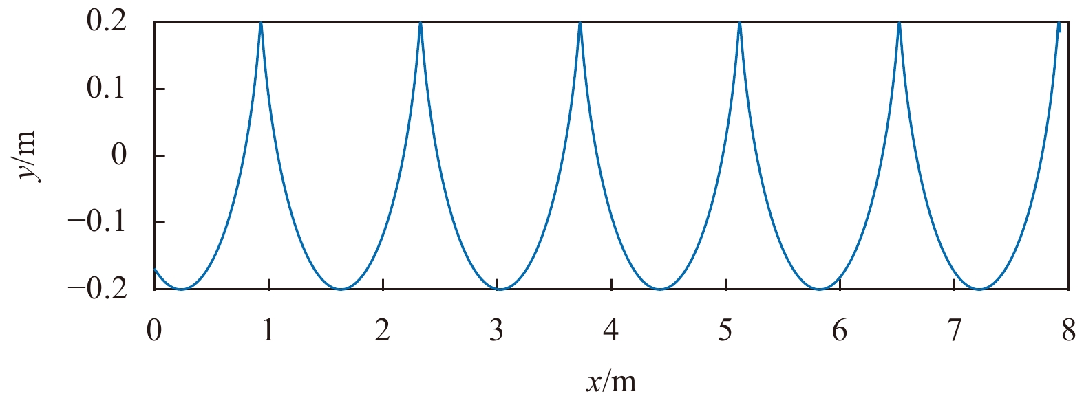
The early research on sea surface modeling regarded the sea surface as a superposition of sine waves or cosine waves (simple harmonics, Fig. 3). The model generated in this way is called the Longuet-Higgins model (Longuet-Higgins, 1952). Its expression is:

| $$ T\left(t\right)=\displaystyle\sum _{i}^{n}{a}_{i}{\rm{cos}}\left({\omega}_{i}+{\varepsilon }_{i}\right){,} $$ | (4) |
where
Combined with JONSWAP spectrum,
| $$ {a}_{i}=\sqrt{{S}_{\rm{JONSWAP}}\left(\omega{,}\theta \right){\rm d}\omega{\rm d}\theta }{,} $$ | (5) |
expand Eq. (5) to three-dimension mode:
| $$\begin{split} T\left(x{,}y{,}t\right)=&{\sum _{i}\sum _{j}\sqrt{{S}_{\rm{JONSWAP}}({\omega}_{i}{,}{\theta }_{j}){\rm d}\omega{\rm d}\theta }{\rm{cos}}\Biggr[{\omega}_{i}t-}\\ &{\frac{{{\omega}_{i}}^{2}}{g}(x{\rm{cos}}{\theta }_{j}+y{\rm{sin}}{\theta }_{j})+{\varepsilon }_{i\text{,}j}\Biggr] {,} } \end{split}$$ | (6) |
where
The Gerstner model was first introduced to the field of computer image processing in 1986 by Fournier and Reeves (1986). This model mainly describes the motion state of each particle on the sea surface from the perspective of dynamics, and is generally represented by a parametric equation:
| $$ \left\{\begin{split}&x={x}_{0}-r{\rm{sin}}\left(\frac{{\omega}^{2}}{g}{x}_{0}-\omega t\right),\\ &y={y}_{0}+r{\rm{cos}}\left(\frac{{\omega}^{2}}{g}{y}_{0}-\omega t\right),\end{split}\right. $$ | (7) |
where

Combined with the JONSWAP spectrum,
| $$ r=\sqrt{{S}_{\rm{JONSWAP}}\left(\omega{,}\theta \right){\rm d}\omega{\rm d}\theta }{,} $$ | (8) |
expand Eq. (8) to three-dimension mode:
| $$ \left\{\begin{split}&x={x}_{0}-\\ &\sum _{i}\sum _{j}\sqrt{{S}_{\rm{JONSWAP}}\left({\omega}_{i}{,}{\theta }_{j}\right){\rm d}\omega{\rm d}\theta }{\rm{cos}}{\theta }_{j}\times\\ &{\rm{sin}}\left[\frac{{\omega}^{2}}{g}\left({x}_{0}{\rm{cos}}{\theta }_{j}+{y}_{0}{\rm{sin}}{\theta }_{j}-{\omega}_{i}t+{\varepsilon }_{i{,}j}\right)\right],\\ &y={y}_{0}-\\ &\sum _{i}\sum _{j}\sqrt{{S}_{\rm{JONSWAP}}\left({\omega}_{i}{,}{\theta }_{j}\right){\rm d}\omega{\rm d}\theta }{\rm{sin}}{\theta }_{j}\times\\ &{\rm{sin}}\left[\frac{{\omega}^{2}}{g}\left({x}_{0}{\rm{cos}}{\theta }_{j}+{y}_{0}{\rm{sin}}{\theta }_{j}-{\omega}_{i}t+{\varepsilon }_{i{,}j}\right)\right],\\ &z=\\ &\sum _{i}\sum _{j}\sqrt{{S}_{\rm{JONSWAP}}\left({\omega}_{i}{,}{\theta }_{j}\right){\rm d}\omega{\rm d}\theta }\\ &{\rm{cos}}\left[\frac{{\omega}^{2}}{g}\left({x}_{0}{\rm{cos}}{\theta }_{j}+{y}_{0}{\rm{sin}}{\theta }_{j}-{\omega}_{i}t+{\varepsilon }_{i{,}j}\right)\right],\end{split}\right. $$ | (9) |
where
Chen (2013) compared the commonly used seismic wave equation with the water wave model construction method based on the principle of fluid dynamics, and assumed that fluid is inviscid and incompressible, comparing the two equations:
| $$ \begin{split} \frac{{\rm d}^{2}h\left(x{,}y{,}t\right)}{{\rm d}{t}^{2}}=gp\left(\frac{{\rm d}^{2}h\left(x{,}y{,}t\right)}{{\rm d}{x}^{2}}+\frac{{\rm d}^{2}h\left(x{,}y{,}t\right)}{{\rm d}{y}^{2}}\right){,}\;\; h\left(x{,}y{,}{t}_{0}\right)={h}_{0}, \end{split}$$ | (10) |
where
In addition, the commonly used seismic wave equation is given:
| $$ \frac{{\rm d}^{2}u\left(x{,}y{,}t\right)}{{\rm d}{t}^{2}}={v}^{2}\left(\frac{{\rm d}^{2}u\left(x{,}y{,}t\right)}{{\rm d}{x}^{2}}+\frac{{\rm d}^{2}u\left(x{,}y{,}t\right)}{{\rm d}{y}^{2}}\right){,} $$ | (11) |
where
It can be found that the two equations are similar. Therefore, the algorithms related to seismic wave numerical simulation can be applied to the calculation of sea surface. The finite difference method is used here.
First, discretize Eq. (10) and find the difference format:
| $$ \begin{split} h(x{,}y{,}t + 1) = &{2h(x{,}y{,}t) - h(x{,}y{,}t - }1) + \\ &\frac{{gp\Delta {t^2}}}{{\Delta {x^2}}}[h({{x}} + 1{,}y{,}t) - 2h(x{,}y{,}t) + \\ &{h(x - 1{,}y{,}t)] + \frac{{gp\Delta {t^2}}}{{\Delta {y^2}}}[h(x{,}y + 1{,}t) - }\\ &{2h(x{,}y{,}t) + h(x{,}y - 1{,}t)]{,}} \end{split}$$ | (12) |
where
| $$ \begin{split} h(x{,}y{,}t + 1) =&{ 2h(x{,}y{,}t) - h(x{,}y{,}t - }1)+\\ &{P[h(x + 1{,}y{,}t) - 2h(x{,}y{,}t) + }\\ &{h(x - 1{,}y{,}t)] + P[h(x{,}y + 1{,}t) - }\\ &{2h(x{,}y{,}t) + h(x{,}y - 1{,}t)]{.}} \end{split}$$ | (13) |
To solve this equation, two initial conditions of time steps should be required. The initial conditions can be derived from the model generated by simple harmonics or Gerstner wave, or in other ways.
Chen (2013) discussed the convergence conditions of stable iteration of Eq. (13) and conclude that when
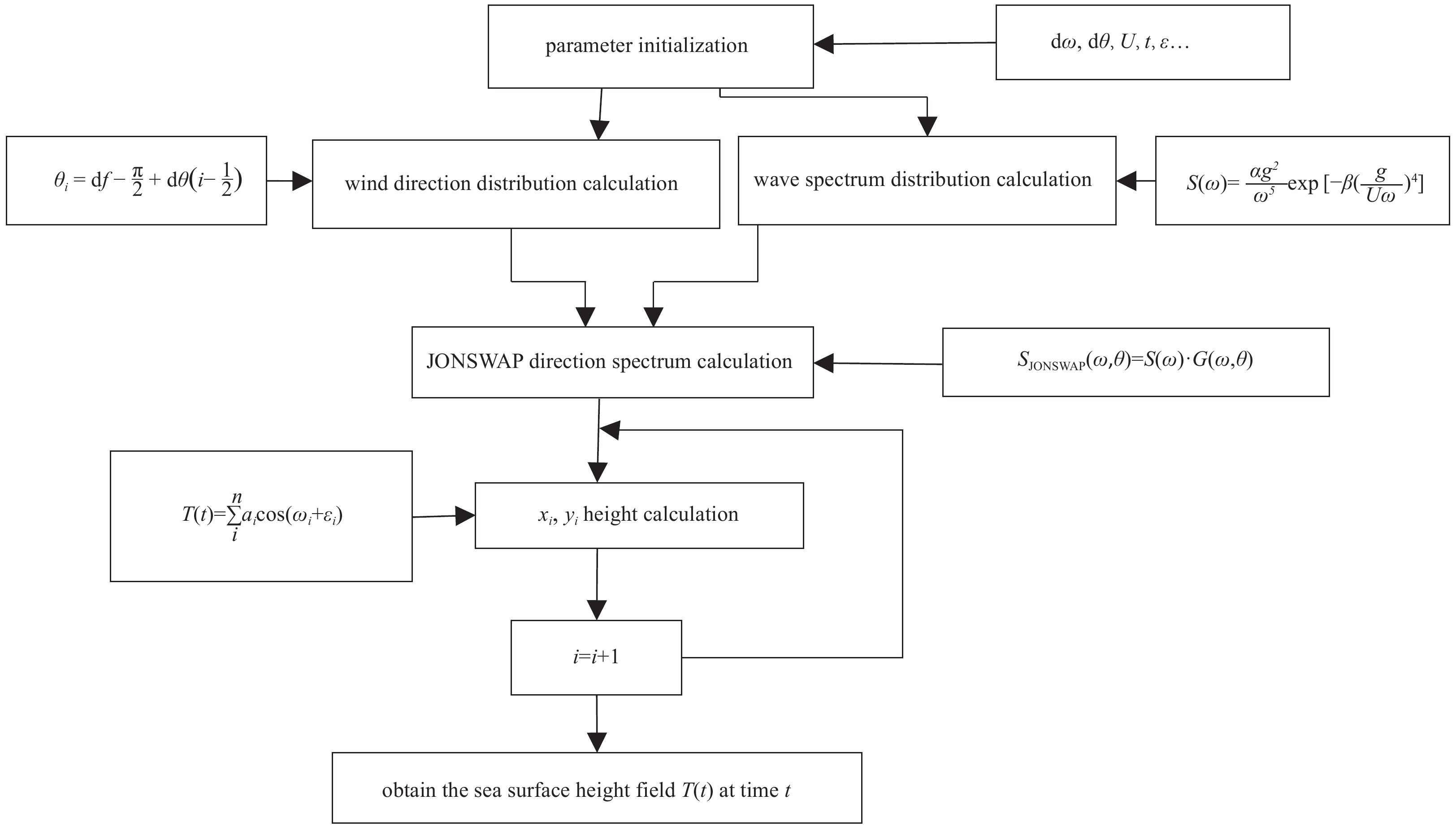
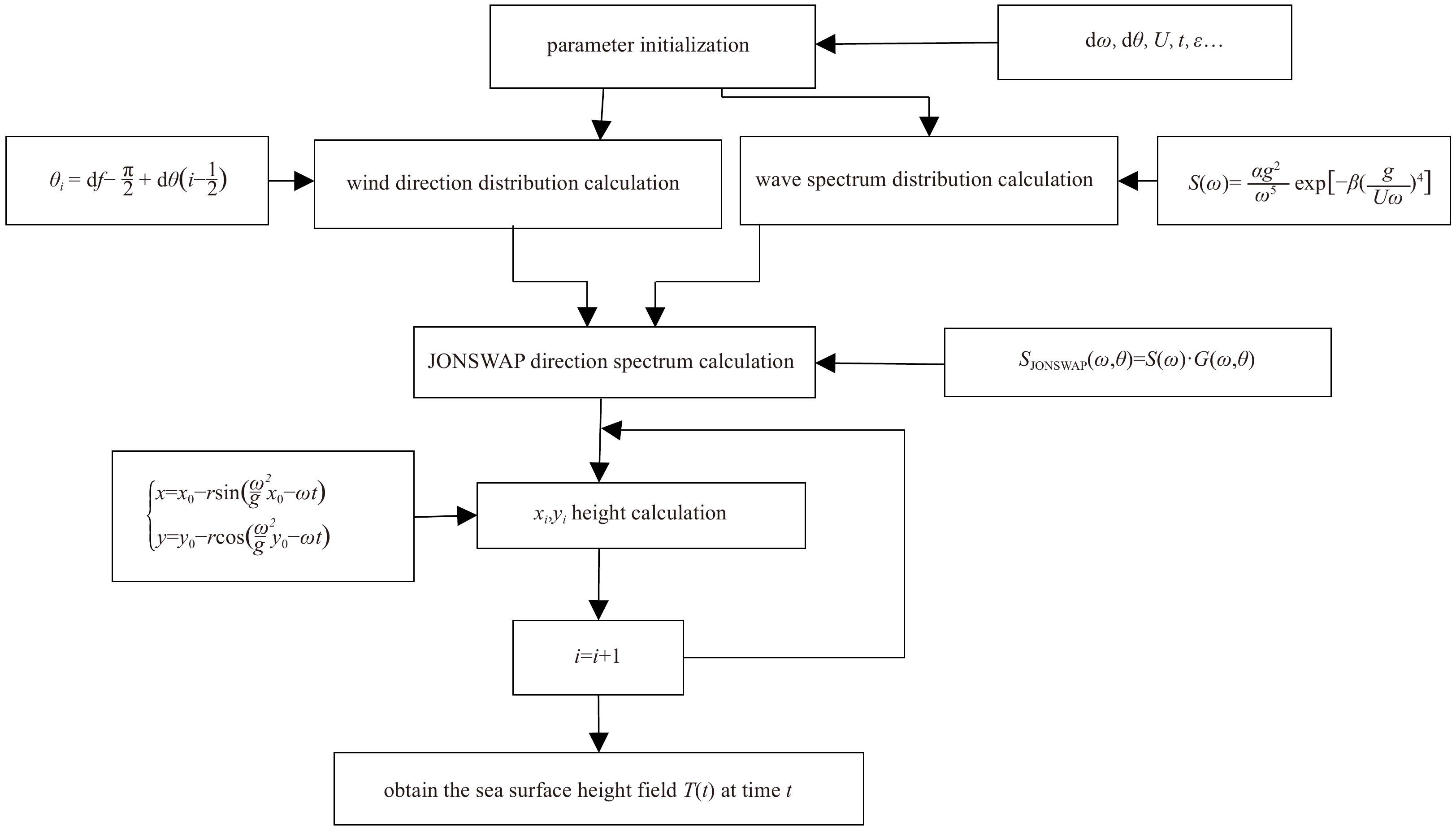
In addition to the theoretical equation derivation of the three ways mentioned above, the simulation process and parameter selection also need to be explained in the specific implementation process. Next, the specific implementation steps of the three simulation ways will be explained separately (Fig. 5).

| Parameters | Value |
| Wind speed $ U $ at 19.5 m above sea surface | 8 m/s |
| Wind direction df | π/3 |
| Wind direction division number $ m $ | 30 |
| Wind direction interval $ {\rm d}\theta $ | 2π/m |
| Frequency interval ${\rm d} {\omega}$ | π/100 |
| Computational grid | $ 100\times 100 $ |
| Time step | 1 s |
 DownLoad:
CSV
DownLoad:
CSV
Table 1 shows the simulation parameter value below.
Within the specified range, divide the
| $$ {\theta }_{i}={\rm d}f-\frac{\pi }{2}+{\rm d}\theta \left(i-\frac{1}{2}\right){,} $$ | (14) |
where
Substituting Eq. (14) into Eq. (3) and combining it with Eq. (2),
| $$ \begin{split} &{{S}_{\rm{JONSWAP}}\left(\omega{,}\theta \right)=\frac{\alpha {g}^{2}}{{\omega}^{5}}\exp\left[-\mathrm{\beta }{\left(\frac{g}{U\omega}\right)}^{4}\right]\times}\\ &{\frac{1}{\pi }\left[1+p{\rm{cos}}\left(2\theta \right)+q{\rm{cos}}\left(4\theta \right)\right]{.}} \end{split} $$ | (15) |
Substituting Eq. (15) into Eq. (6), the height at each point can be calculated. And the simulation results are shown in Fig. 6.

The simulation process using Gerstner waves is basically the same as that of simple harmonics (Fig. 7). After Eq. (15) is obtained, Eq. (9) is substituted for calculation according to the time steps. And the simulation results are shown in Fig. 8.


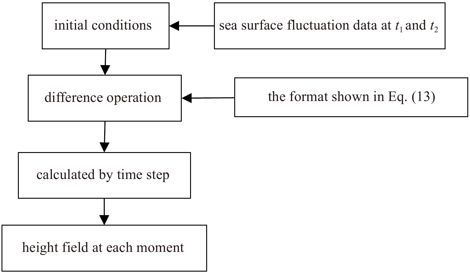
In order to use the different formats of the wave equation to calculate the real-time condition of the sea surface, two conditions are required (Fig. 9). The first is to collect several consecutive moments of sea surface (i.e., the initial conditions), and the second is to require a suitable

According to Chen’s (2013) research results, the value of
The sea surface at a continuous moment can be obtained by any of the above ways. After obtaining the sea surface undulation matrix, substituting it into Eq. (13), then forward according to the time steps can be calculated. And the simulation results are shown in Fig. 10.

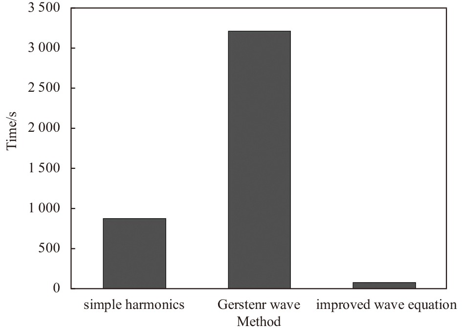
In order to show the difference between the three ways, it is necessary to compare the calculation speed and the model realization effect.
The computer hardware and software conditions for calculation are: Ubuntu 20.04.1 LTS, Core i7-6700 3.40GHz processor, and the wave spectrum uses full frequency calculation. The calculation speed comparison is shown in Table 2.
| Model | Simple harmonic | Gerstner wave | Wave equation |
| Time required to calculate 100 groups/s | 876. 77 | 3 216. 19 | 74.02 |
DownLoad:
CSV
Comparing the calculation speed of the above three simulation methods, the wave equation is the fastest, the simple harmonic is the second, and the Gerstner wave is the slowest. From the perspective of algorithm time complexity, for the wave equation method, since only Eq. (13) needs to be calculated, and Eq. (13) is a linear expression, the complexity is the lowest; for simple harmonics, this method involves a trigonometric function operation, so the complexity is higher; for Gerstner wave method, compared with the simple harmonic, at least three operations with the same complexity as the simple harmonic have been experienced, so the complexity is higher.
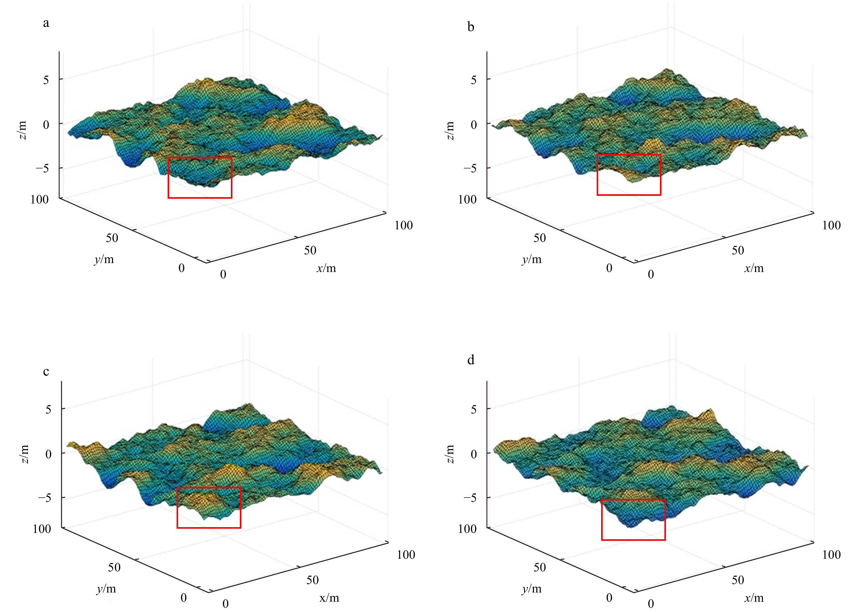
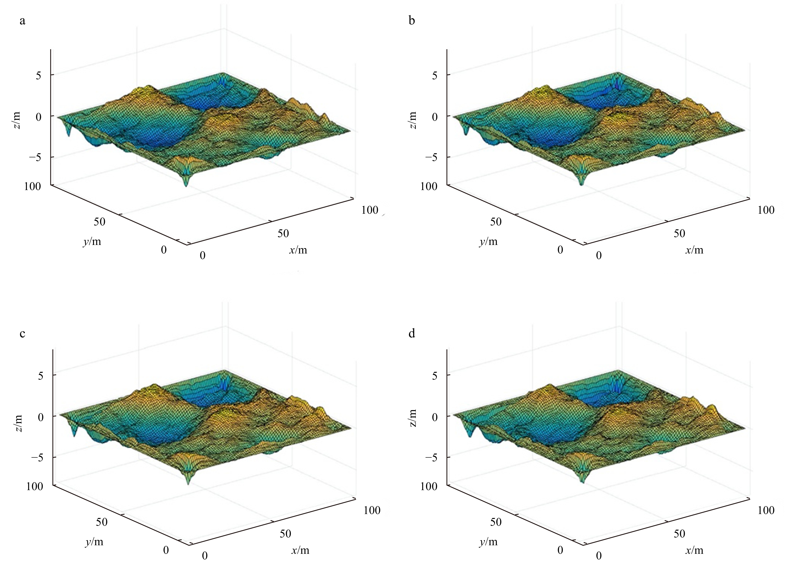
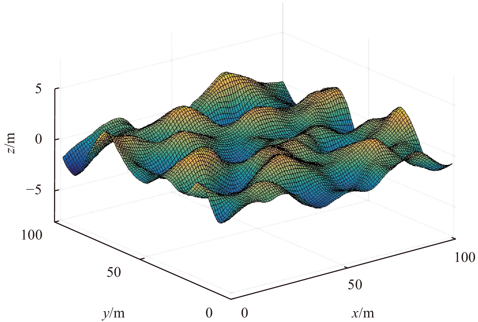
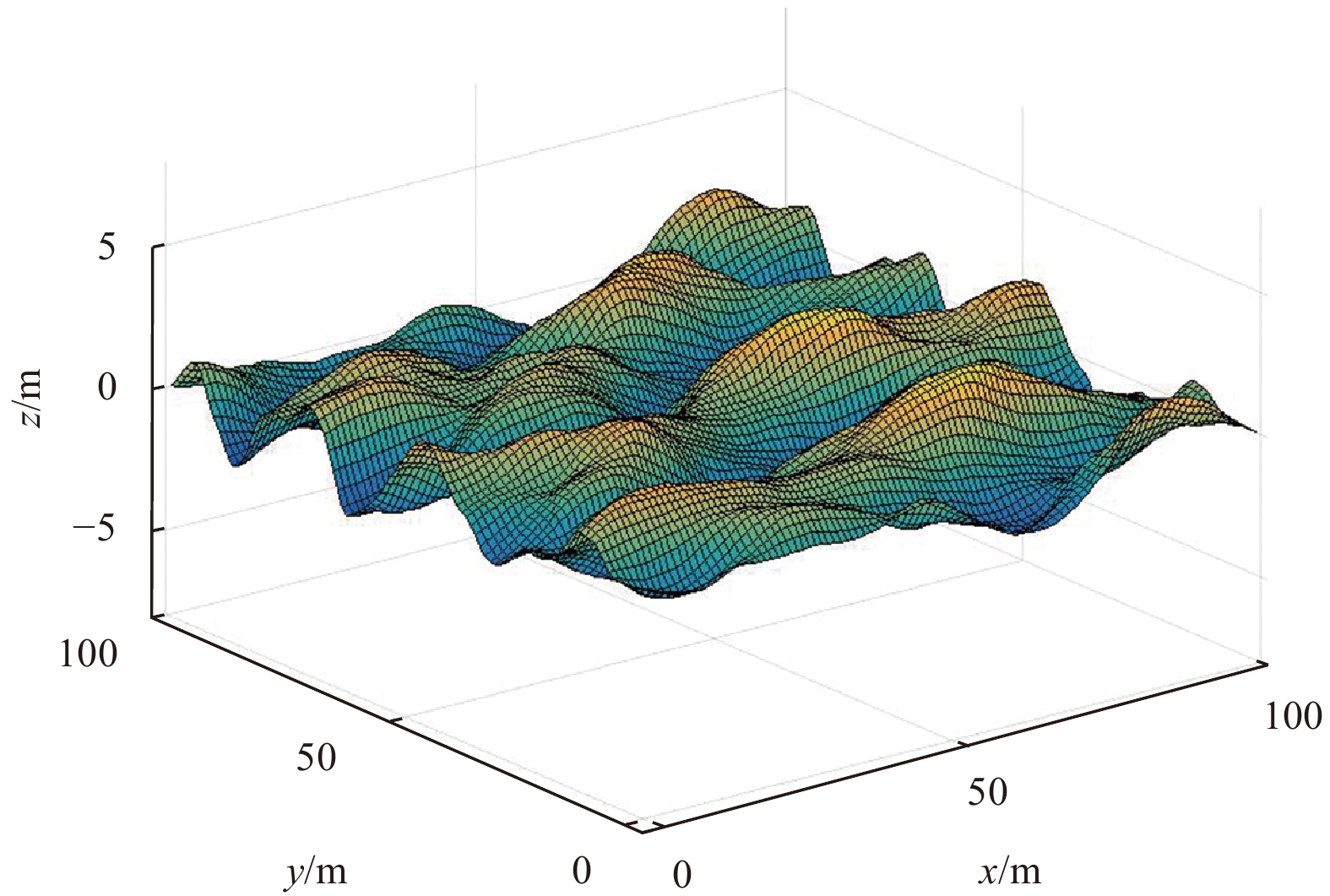
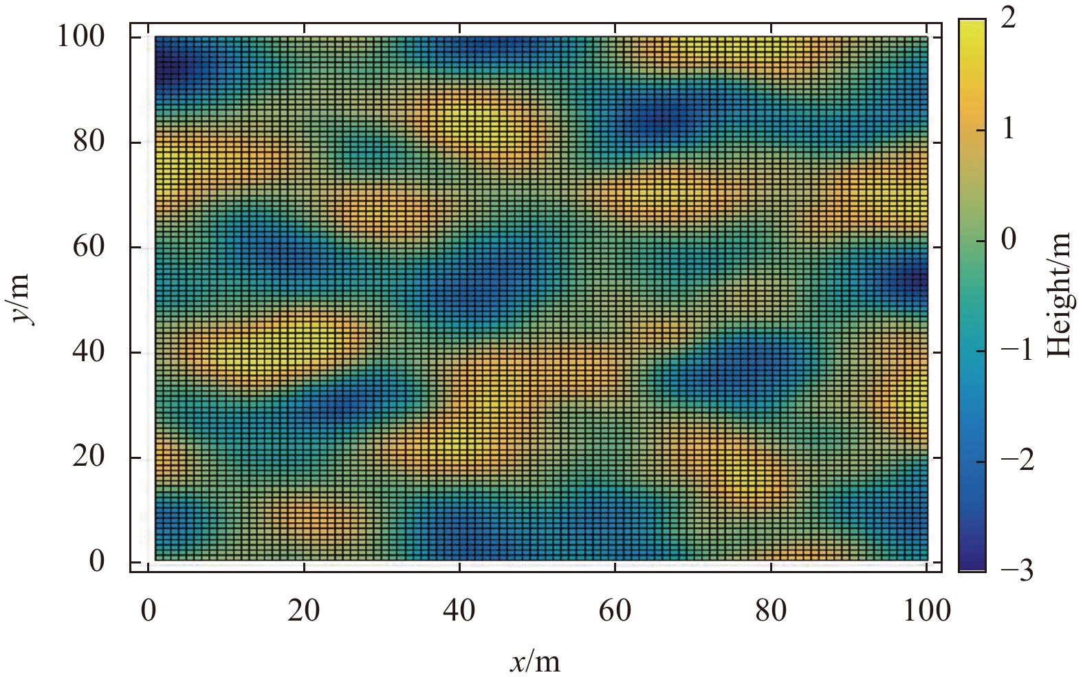
The sea surface drawn by simple harmonics is shown in Fig. 11. The sea surface characteristics simulated by the simple harmonic method are that the peaks and valleys are relatively discontinuous (mainly compared with Gerstner method). On the image created by the Gerstner method (Fig. 12), the continuous wave crests with lines have been marked, but in Fig. 11, you could not find such a continuous line. This way can better show the ups and downs of the sea. You can see the ups and downs in Fig. 6. One of the positions was circled with a box, and you can observe this wave crest, which is changing up and down over time (of course it is not in one position, other positions are the same ups and downs).


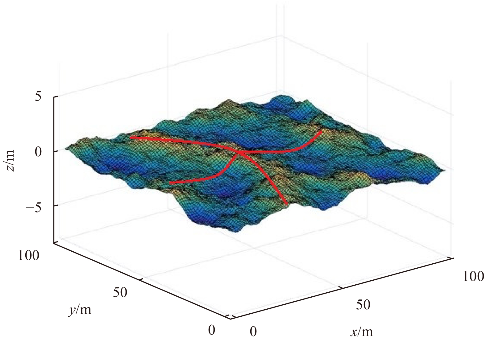
The sea surface characteristics simulated by the Gerstner wave method are that the sharp parts of the waves can be well represented. In fact, the sea surface described in this way is more in line with the physical characteristics of the actual sea surface (Liu et al., 2006) (Fig. 12). In addition, the Gerstner way has a better simulation effect than simple harmonics when describing the propulsion of ocean waves. The effect of wave crest advancement can be clearly seen in Fig. 8. One of the wave crests has been marked with a box, and can clearly observe that this wave crest is constantly moving forward as time goes by.
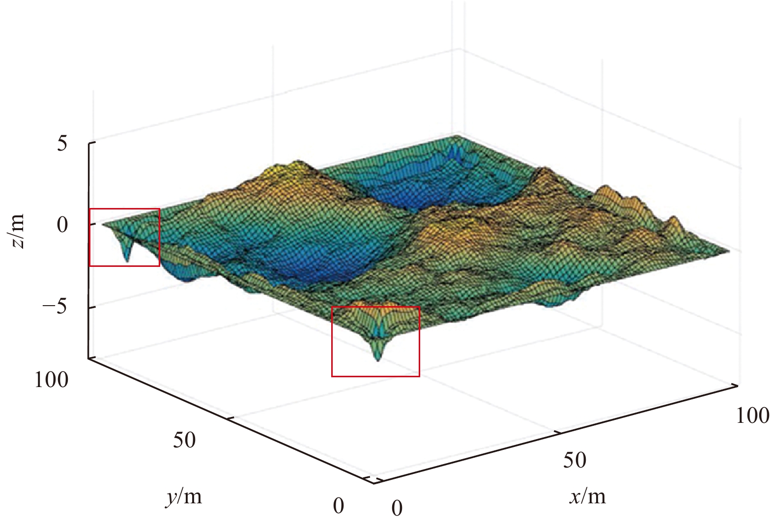
The nature of the wave equation method to simulate the sea surface is the law of seismic wave propagation. Therefore, problems in the calculation of the difference in seismic wave propagation will also appear here, such as boundary effects, the obvious boundary effect will be seen at the mark in Fig. 13; in addition, since the wave equation way only contains wind speed and direction information under initial conditions. As the calculation steps, the accuracy of the results will become lower and lower (Fig. 10).

The simple harmonic, Gerstner wave and wave equation have their respective application ranges. The simple harmonic method is suitable for describing the undulating sea surface with weak wind. The Gerstner wave is suitable for describing the advancement of ocean waves. The wave equation is suitable for algorithm that involves sea surface undulations when conditions such as wind and waves are not required. Although the former two can simulate a more realistic sea surface, when simulating a large range of dynamic sea surface, it consumes a lot of calculation time.
In order to take into account the calculation time and the model simulation effect, this paper proposes an improved method of dynamic sea surface modeling based on wave equation, so that it can simulate a more realistic dynamic sea surface with almost no loss of calculation speed.
The wave equation way represented by Eq. (13) essentially does not fully utilize the wave spectrum, and does not include information such as wind force and wind direction in the calculation. Considering starting from the boundary conditions, the dynamic boundary conditions containing wave spectrum information will be derived, and modeling the undulating sea surface based on this.
Assuming that the coordinate of a point
| $$ {P}_{zi}=r{\rm{sin}}(\omega t+e){,} $$ | (16) |
where
The energy intensity
| $$ r=\sqrt{{S}_{\rm{JONSWAP}}\left(\omega{,}\theta \right){\rm d}\omega{\rm d}\theta } .$$ |
For each moving point, each frequency of the wave spectrum corresponds to a simple harmonic motion. For this point,
| $$ \begin{split} &{ {P}_{i1}=\sqrt{{S}_{\rm{JONSWAP}}\left({\omega}_{1}{,}\theta \right){\rm d}\omega{\rm d}\theta }\sin({\omega}_{1}t+{e}_{1})},\\ &{{P}_{i2}=\sqrt{{S}_{\rm{JONSWAP}}\left({\omega}_{2}{,}\theta \right){\rm d}\omega{\rm d}\theta }\sin({\omega}_{2}t+{e}_{2})},\\ &{ \cdots }\\ &{{P}_{in}=\sqrt{{S}_{\rm{JONSWAP}}\left({\omega}_{n}{,}\theta \right){\rm d}\omega{\rm d}\theta }\sin({\omega}_{n}t+{e}_{n}) }. \end{split} $$ |
Sum the above equations:
| $$\begin{split} { {P}_{i}=\sum _{j}\sqrt{{S}_{\rm{JONSWAP}}\left({\omega}_{j}{,}\theta \right){\rm d}\omega{\rm d}\theta }\sin({\omega}_{j}t+}{{e}_{j}).} \end{split} $$ | (17) |
In order to ensure that all the points that meet the conditions are also continuity along the x-axis, it is necessary to convert Eq. (17) into a two-dimension form, which is:
| $$\begin{split} {h\left(x{,}1{,}t\right)=}&{\sum _{i}\sum _{j}\sqrt{{S}_{\rm{JONSWAP}}\left({\omega}_{i}{,}{\theta }_{j}\right){\rm d}\omega{\rm d}\theta }{\rm{cos}}({\omega}_{i}t-}\\ &{\frac{{{\omega}_{i}}^{2}}{g}\left(x{\rm{cos}}{\theta }_{j}+{\rm{sin}}{\theta }_{j})+{\varepsilon }_{i,j}\right){.}} \end{split} $$ | (18) |
The form of Eqs (18) and (6) is almost the same.
Equation (18) is the lower boundary condition in the wave equation method to simulate the sea surface. When the boundary is upwind, the remaining boundary does not need to substituted into this condition.
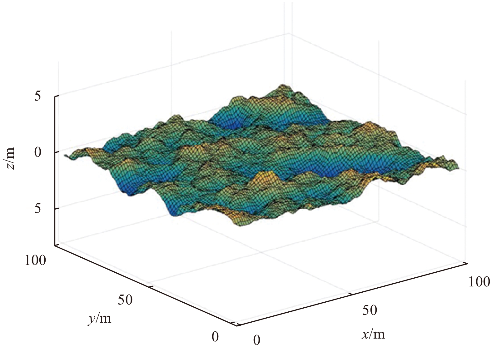
Figure 14 shows the simulation process. Under the same hardware and software conditions, the time required to calculate 100 sets of data using this method is only 81.67 s. From Fig. 15, the effect of the wave advances with time can be seen; since the boundary conditions change with time and will not disappear, if a long-term simulation is to be performed, it is necessary to add absorption boundary on other boundaries. From Fig. 16, the difference in the calculation speed of the three methods can be seen. Obviously, the calculation speed of the improved wave equation method is much slower than other methods.


In order to illustrate the simulation effect of the wave equation method, this method is compared with the sea surface simulated by the high-order spectrum method. The three-dimensional sea surface simulated by the high-order spectrum method used in this article is generated by the open-source high-order spectrum wide-area sea surface solver HOS ocean (Ducrozet et al., 2016), and is displayed by Matlab. The two simulation diagrams are shown in the figures (Figs 17 and 18; and the top views of the figures, Figs 19 and 20).


Compared with the sea surface described by the wave equation method, the wave peaks and troughs have no continuous characteristics compared with those described by the high-order spectrum method, which can be better seen from the top view.
The wave equation method is smoother, and the higher-order spectrum method is sharper at the peaks and valleys.
The wave equation method describes the sea surface lower, and the high-order spectrum method describes the sea surface wave peak higher.
In this paper, three mathematical simulation methods of undulating seas are studied, the implementation process of the three methods is studied in detail, and the differences of the three methods are compared in terms of calculation speed and model effect. From the perspective of the implementation effects, the simple harmonic is suitable for describing the undulating state of the sea under a wide range and weak wind conditions; the Gerstner wave is suitable for describing the local and propelled sea conditions; when extremely fast calculation speed is required or when there is little requirement for the sea level to change with time, the wave equation method can be used. In practical applications, different methods can be used to simulate the sea surface according to different needs. In this paper, the wave equation method is improved, and dynamic boundary conditions containing wave spectrum parameters are added, which makes the calculation speed faster. And by comparing the improved the wave equation and high-order spectral methods, it shows that the sea surface described by the wave equation method is smoother and so on.
In marine seismic exploration, the impact of dynamic sea surface fluctuations cannot be ignored. The premise of studying the impact of sea surface fluctuations is to simulate a more realistic dynamic sea surface condition. This paper explains several sea surface simulation methods from the perspective of mathematical statistics. These methods are more compatible with the model design of seismic wave numerical simulation. The wave equation sea surface simulation under dynamic boundary conditions proposed in this paper can better demonstrate the dynamic sea surface fluctuations, and the calculation speed is faster, which effectively improves the dynamic sea surface generation efficiency. It provides an effective way for wave field simulation model design.
| [1] |
Cecconello E, Asgedom E G, Orji O C, et al. 2018. Modeling scattering effects from time-varying sea surface based on acoustic reciprocity. Geophysics, 83(2): T49–T68. doi: 10.1190/geo2017-0410.1
|
| [2] |
Chen Keyang. 2013. 3D water motion simulation based on wave equation. Journal of Beijing Union University (in Chinese), 27(3): 86–88
|
| [3] |
Cote L J. 1960. The directional spectrum of a wind generated sea as determined from data obtained by the stereo wave observation project [dissertation]. New York: New York University, 88
|
| [4] |
Dommermuth D G, Yue D K P. 1987. A high-order spectral method for the study of nonlinear gravity waves. Journal of Fluid Mechanics, 184: 267–288. doi: 10.1017/S002211208700288X
|
| [5] |
Ducrozet G, Bonnefoy F, Le Touzé D, et al. 2016. HOS-ocean: open-source solver for nonlinear waves in open ocean based on high-order spectral method. Computer Physics Communications, 203: 245–254. doi: 10.1016/j.cpc.2016.02.017
|
| [6] |
Fournier A, Reeves W T. 1986. A simple model of ocean waves. ACM SIGGRAPH Computer Graphics, 20(4): 75–84. doi: 10.1145/15886.15894
|
| [7] |
Hasselmann K. 1973. Measurements of wind-wave growth and swell decay during the Joint North Sea Wave Project (JONSWAP). Hamburg, Germany: Deutches Hydrographisches Institut, 8
|
| [8] |
Hasselmann K, Sell W, Ross D B, et al. 1976. A parametric wave prediction model. Journal of Physical Oceanography, 6(2): 200–228. doi: 10.1175/1520-0485(1976)006<0200:APWPM>2.0.CO;2
|
| [9] |
Laws R, Kragh E. 2002. Rough seas and time-lapse seismic. Geophysical Prospecting, 50(2): 195–208. doi: 10.1046/j.1365-2478.2002.00311.x
|
| [10] |
Li Sujun, Song Hanchen, Wu Lingda. 2006. Real-time modeling and rendering of ocean waves in digital naval battlefields. Journal of System Simulation (in Chinese), 18(S1): 255–257, 259
|
| [11] |
Liu Yingzhong, Liu Hedong, Miao Guoping, et al. 1998. Numerical simulation on water waves by NS equations. Journal of Shanghai Jiaotong University (in Chinese), 32(11): 1–7
|
| [12] |
Liu Jie, Zou Beiji, Zhou Jieqiong, et al. 2006. Modeling Gerstner waves based on the ocean wave spectrum. Computer Engineering and Science (in Chinese), 28(2): 41–44
|
| [13] |
Longuet-Higgins M S. 1952. On the statistical distribution of the heights of sea waves. Journal of Marine Research, 11(3): 245–266
|
| [14] |
Meng Xiangyu, Sun Jianguo, Wei Puli, et al. 2019. Undulating sea surface influence on reflection seismic responses. Oil Geophysical Prospecting (in Chinese), 54(4): 787–795
|
| [15] |
Monaghan J J. 2005. Smoothed particle hydrodynamics. Reports on Progress in Physics, 68(8): 1703–1759. doi: 10.1088/0034-4885/68/8/R01
|
| [16] |
Phillips O M. 1958. The equilibrium range in the spectrum of wind-Generated waves. Journal of Fluid Mechanics, 4(4): 426–434. doi: 10.1017/S0022112058000550
|
| [17] |
Pierson W J Jr, Moskowitz L. 1964. A proposed spectral form for fully developed wind seas based on the similarity theory of S. A. Kitaigorodskii. Journal of Geophysical Research, 69(24): 5181–5190. doi: 10.1029/JZ069i024p05181
|
| [18] |
Qi Peng. 2015. Seismic wave modeling under the complex marine conditions (in Chinese)[dissertation]. Changchun: Jilin University
|
| [19] |
Qi Ning, Xia Tian, Li Wenyan, et al. 2013. Simulation of the mathematical model of 3-D irregular wave based on MATLAB. Computer Knowledge and Technology (in Chinese), 9(25): 5737–5739
|
| [20] |
Shen Yanming, Shi Wenkui, Chen Jianqiang, et al. 2020. Application of SPH method with space-based variable smoothing length to water entry simulation. Journal of Ship Mechanics (in Chinese), 24(3): 323–331
|
| [21] |
Sun Xiaoyan, Wang Jun. 2007. Theories and application on Smoothed Particle Hydrodynamics method. Water Resources and Hydropower Engineering (in Chinese), 38(3): 44–46
|
| [22] |
Wang Xianhua, Peng Zhaohui, Li Zhenglin. 2007. Effects of wave fluctuation on sound propagation. Technical Acoustics (in Chinese), 26(4): 551–556
|
| [23] |
Wu Chengsheng, Zhu Dexiang, Gu Min. 2008. Simulation of radiation problem moving with forward speed by solving N-S equations. Journal of Ship Mechanics (in Chinese), 12(4): 560–567
|
| [24] |
Zhang Sijiang, Yang Jie, Ouyang Yi. 2013. 3D numerical simulation of sea wave based on directional spectrum. Shipboard Electronic Countermeasure (in Chinese), 36(4): 54–57
|
| 1. | Lianwei Li, Shiyu Wu, Cunjin Xue, et al. Research on Visualization Methods for Marine Environmental Element Fields in Twin Spaces. Journal of Marine Science and Engineering, 2025, 13(3): 449. doi:10.3390/jmse13030449 | |
| 2. | Yao He, Le Xu, Jincong Huo, et al. A Synthetic Aperture Radar Imaging Simulation Method for Sea Surface Scenes Combined with Electromagnetic Scattering Characteristics. Remote Sensing, 2024, 16(17): 3335. doi:10.3390/rs16173335 | |
| 3. | Xi Duan, Jian Liu, Xinjie Wang. Real-Time Wave Simulation of Large-Scale Open Sea Based on Self-Adaptive Filtering and Screen Space Level of Detail. Journal of Marine Science and Engineering, 2024, 12(4): 572. doi:10.3390/jmse12040572 | |
| 4. | Wenhao Gan, Xiuqing Qu, Dalei Song, et al. Multi-USV Cooperative Chasing Strategy Based on Obstacles Assistance and Deep Reinforcement Learning. IEEE Transactions on Automation Science and Engineering, 2024, 21(4): 5895. doi:10.1109/TASE.2023.3319510 | |
| 5. | Xiangzhi Cheng, Xixiang Liu, Xiaoqiang Wu, et al. An inertial alignment and linear motion separation method of unmanned offshore platform based on parameter identification. Ocean Engineering, 2024, 311: 118883. doi:10.1016/j.oceaneng.2024.118883 | |
| 6. | Shuxian Huang, Li Huang, Xin Ning. CLO3D-Based 3D Virtual Fitting Technology of Down Jacket and Simulation Research on Dynamic Effect of Cloth. Wireless Communications and Mobile Computing, 2022, 2022: 1. doi:10.1155/2022/5835026 | |
| 7. | Chen Wu, Rui Zhao, He Yan, et al. The inversion of ocean current extraction by along-track interferometric SAR based on sea surface model. Third International Conference on Advanced Algorithms and Signal Image Processing (AASIP 2023), doi:10.1117/12.3006132 | |
| 8. | Jiayue Liu, Tianqi Mao, Dongxuan He, et al. Reinforcement-Learning-Enabled Beam Alignment for Water-Air Direct Optical Wireless Communications. 2024 IEEE/CIC International Conference on Communications in China (ICCC), doi:10.1109/ICCC62479.2024.10681690 | |
| 9. | Yubo Wen, Ping Wang, Huadong Ma, et al. Research and Application of Integrated Simulation Technology for Surface and Subsurface Waters in the Guangdong-Hong Kong-Macao Greater Bay Area. 2024 9th International Symposium on Computer and Information Processing Technology (ISCIPT), doi:10.1109/ISCIPT61983.2024.10672872 | |
| 10. | Jianlong Wang, Zhongxun Wang, Yujie Chen, et al. Improved Gerstner Function Wave Model Based on Elfouhaily Spectrum. 2024 Global Reliability and Prognostics and Health Management Conference (PHM-Beijing), doi:10.1109/PHM-Beijing63284.2024.10874818 |

Figures(20) / Tables(2)

Supported by:
Beijing Renhe Information Technology Co. Ltd

Zhimiao Chang, Fuxing Han, Zhangqing Sun, Zhenghui Gao, Lili Wang. Three-dimensional dynamic sea surface modeling based on ocean wave spectrum[J]. Acta Oceanologica Sinica, 2021, 40(10): 38-48. doi: 10.1007/s13131-021-1871-6

| Parameters | Value |
| Wind speed $ U $ at 19.5 m above sea surface | 8 m/s |
| Wind direction df | π/3 |
| Wind direction division number $ m $ | 30 |
| Wind direction interval $ {\rm d}\theta $ | 2π/m |
| Frequency interval ${\rm d} {\omega}$ | π/100 |
| Computational grid | $ 100\times 100 $ |
| Time step | 1 s |
DownLoad:
CSV
| Model | Simple harmonic | Gerstner wave | Wave equation |
| Time required to calculate 100 groups/s | 876. 77 | 3 216. 19 | 74.02 |
DownLoad:
CSV
| Parameters | Value |
| Wind speed $ U $ at 19.5 m above sea surface | 8 m/s |
| Wind direction df | π/3 |
| Wind direction division number $ m $ | 30 |
| Wind direction interval $ {\rm d}\theta $ | 2π/m |
| Frequency interval ${\rm d} {\omega}$ | π/100 |
| Computational grid | $ 100\times 100 $ |
| Time step | 1 s |
| Model | Simple harmonic | Gerstner wave | Wave equation |
| Time required to calculate 100 groups/s | 876. 77 | 3 216. 19 | 74.02 |
 DownLoad:


 DownLoad: