Ruibin Xia, Yijun He, Tingting Yang. Simulation and future projection of the mixed layer depth and subduction process in the subtropical Southeast Pacific[J]. Acta Oceanologica Sinica, 2021, 40(12): 104-113. doi: 10.1007/s13131-021-1877-0
Citation:
Ruibin Xia, Yijun He, Tingting Yang. Simulation and future projection of the mixed layer depth and subduction process in the subtropical Southeast Pacific[J]. Acta Oceanologica Sinica, 2021, 40(12): 104-113. doi: 10.1007/s13131-021-1877-0
Ruibin Xia, Yijun He, Tingting Yang. Simulation and future projection of the mixed layer depth and subduction process in the subtropical Southeast Pacific[J]. Acta Oceanologica Sinica, 2021, 40(12): 104-113. doi: 10.1007/s13131-021-1877-0
Citation:
Ruibin Xia, Yijun He, Tingting Yang. Simulation and future projection of the mixed layer depth and subduction process in the subtropical Southeast Pacific[J]. Acta Oceanologica Sinica, 2021, 40(12): 104-113. doi: 10.1007/s13131-021-1877-0
School of Marine Sciences, Nanjing University of Information Science and Technology, Nanjing 210044, China
2.
MNR Key Laboratory for Polar Science, Polar Research Institute of China, Shanghai 200136, China
3.
Laboratory for Regional Oceanography and Numerical Modeling, Pilot National Laboratory for Marine Science and Technology (Qingdao), Qingdao 266237, China
4.
Key Laboratory of Meteorological Disaster, Ministry of Education, Nanjing 210044, China
5.
Joint International Research Laboratory of Climate and Environment Change, Nanjing 210044, China
6.
Collaborative Innovation Center on Forecast and Evaluation of Meteorological Disasters, Nanjing 210044, China
7.
Nanjing Joint Institute for Atmospheric Sciences, Nanjing 210008, China
Funds:
The National Natural Science Foundation of China under contract Nos 41606217 and 41620104003; the Open Fund of Key Laboratory for Polar Science, Polar Research Institute of China, Ministry of Natural Resources, under contract No. KP201702; the Open Fund of the Key Laboratory of Ocean Circulation and Waves, Chinese Academy of Sciences, under contract No. KLOCW1903.
The present climate simulation and future projection of the mixed layer depth (MLD) and subduction process in the subtropical Southeast Pacific are investigated based on the geophysical fluid dynamics laboratory earth system model (GFDL-ESM2M). The MLD deepens from May and reaches its maximum (>160 m) near (24°S, 104°W) in September in the historical simulation. The MLD spatial pattern in September is non-uniform in the present climate, which shows three characteristics: (1) the deep MLD extends from the Southeast Pacific to the West Pacific and leads to a “deep tongue” until 135°W; (2) the northern boundary of the MLD maximum is smoothly near 18°S, and MLD shallows sharply to the northeast; (3) there is a relatively shallow MLD zone inserted into the MLD maximum eastern boundary near (26°S, 80°W) as a weak “shallow tongue”. The MLD non-uniform spatial pattern generates three strong MLD fronts respectively in the three key regions, promoting the subduction rate. After global warming, the variability of MLD spatial patterns is remarkably diverse, rather than deepening consistently. In all the key regions, the MLD deepens in the south but shoals in the north, strengthing the MLD front. As a result, the subduction rate enhances in these areas. This MLD antisymmetric variability is mainly influenced by various factors, especially the potential-density horizontal advection non-uniform changes. Notice that the freshwater flux change helps to deepen the MLD uniformly in the whole basin, so it hardly works on the regional MLD variability. The study highlights that there are regional differences in the mechanisms of the MLD change, and the MLD front change caused by MLD non-uniform variability is the crucial factor in the subduction response to global warming.
The subtropical Pacific (SEP) has long been recognized as an important region for climate studies because subsurface signals propagate towards the tropics (Gu and Philander, 1997; Wang and Luo, 2020). The subsurface temperature/salinity anomalies in the SEP can be formed locally through subduction and injection processes, both depend on the mixed layer process (Williams, 1991; Qiu and Huang, 1995; Sato and Suga, 2009; Wang and Luo, 2020). The ocean mixed layer depth (MLD) is one of the most important quantities of the upper ocean as it defines the quasi-homogeneous surface region of density that directly interacts with the atmosphere (Kara et al., 2003). Atmospheric fluxes of momentum, heat and freshwater through the ocean surface drive vertical mixing and provide the source of almost all oceanic motions (de Boyer Montégut et al., 2004; Dong et al., 2008).
There is a region with local maximum MLD (>100 m) in the SEP in austral winter, with a strong MLD front and the corresponding subduction process on the north side, where the South Pacific eastern subtropical mode water (SPESTMW) forms (Wong and Johnson, 2003). The SPESTMW is significantly stronger than the eastern North Pacific subtropical mode water (ESTMW) in the present climate. The SPESTMW could potentially affect the El Niño-Southern Oscillation (ENSO) cycle through the interior communication window. Several mechanisms have been proposed to explain mixed layer formation and variability in the SEP (Wong and Johnson, 2003; Carton and Giese, 2008; Sato and Suga, 2009). The temporal variability of the MLD is usually linked to many processes occurring in the mixed layer or near the ocean surface (the sea surface heat/freshwater flux and Ekman pumping, etc.). Besides, some studies focused on the effect of ocean advection. Xie et al. (2010) pointed out that ocean advection influences the SST change after global warming. The intensification of the South Pacific subantarctic mode water (SAMW) is mainly caused by a deepening of the MLD and a strengthening of the advection in a warm climate (Liu and Wang, 2014). With the model simulation results, it is proved that the ocean horizontal temperature advection plays a critical role in the MLD non-uniform pattern in the subtropical Northeast Pacific (Xia et al., 2018). With Argo observations, Liu and Lu (2016) summarized the effects of ocean dynamics on the seasonal MLD variability in the SEP in two aspects: (1) the combined effect of net surface heat flux and meridional density advection by the subtropical gyre determines the northern and southern boundaries of the deeply mixed layer region; (2) zonal density advection by the subtropical countercurrent (STCC) dominates the western boundary of the MLD maximum area, by carrying lighter water to strengthen the stratification and generating a “shallow tongue” of MLD to block the westward extension of the deep mixed layer in the STCC region. Density/temperature advection changes the ocean vertical density/temperature gradient, impacts the ocean stratification, and then contributes to the ocean mixing process. But more detailed analyses about the mixed layer mechanisms in the SEP are still necessary, especially for the impacts of ocean advection on a long-time scale.
The response of the MLD and subduction rate to global warming is an interesting question, which would influence the mode water change and the subsequent climatical effects in the future. Coincidentally, the ESTMW and SPESTMW tend to decrease and increase in volume respectively, in sharp contrast with each other, after the climate warms (Luo et al., 2009, 2011). A comparison of the MLD spatial patterns from a series of numerical ocean model experiments suggested that the reduction of the ocean-to-atmosphere heat loss and the weakened Ekman pumping rate resulting from a reduction of the basin-wide wind stress may affect the MLD change (Luo et al., 2009). But in the SEP, the intensified southeasterly trade wind, via generating a stronger buoyancy flux from the ocean to the atmosphere, results in a deeper mixed layer in a warmer climate (Luo et al., 2011). Our previous research pointed that the non-uniform MLD change in the Northeast Pacific is dominated by the non-uniform ocean horizontal advection in the present climate (Xia et al., 2018) or after global warming (Xia et al., 2021). The mechanisms of the MLD climatology and response to global warming are regionally independent in the Northeast Pacific, and the ocean surface currents play an important role in the response of the MLD to global warming (Xia et al., 2021). So how the ocean advection impacts the MLD and subduction process in the SEP under the present climate and after global warming? Does the regional diversity of the MLD climatology and response mechanisms exist in the SEP? These questions will be discussed in this paper. We aim to confirm the MLD and subduction climatology characteristics and their response to global warming in the SEP, and then analyze the corresponding mechanisms. We hypothesize the MLD climatology and its variability are also non-uniform, and the regional independence of the dominant factors is important in the SEP.
The rest of the paper is organized as follows. A brief description of the data and methods is introduced in Section 2. We examine the MLD characteristics and changes from the present climate to a warmer future climate and describe its influence on the subduction process in Section 3. The mechanisms of the MLD changes are discussed in Section 4. Finally, Section 5 presents the conclusions and discussion.
2.
Data and methods
2.1
Model and observational data
The present study primarily uses the output from the earth system model (ESM2M) of the National Oceanic and Atmospheric Administration (NOAA) Geophysical Fluid Dynamics Laboratory (GFDL). ESM2M is a global coupled ocean-atmosphere-land-ice model, as one of the Coupled Model Intercomparison Project Phase 5 (CMIP5) models (Dunne et al., 2012; Taylor et al., 2012). ESM2M with pressure-based vertical coordinates has been used along the developmental path of GFDL’s Modular Ocean Model Version 4.1. The model has a horizontal resolution of 1.0°×1.0° and 50 vertical layers (31 layers in the upper 500 m). The zonal resolution increases toward the equator and reaches (1/3)° between 30°S and 30°N. In this model, we choose the historical simulation and the representative concentration pathways (RCP) 8.5 scenarios. The historical simulation simulates the 20th-century climate forced by observed atmospheric composition changes (Taylor et al., 2012). While in the RCP8.5 scenarios, the radiative forcing increases throughout the 21st century and arrives at a level of approximately 8.5 W/m2 at the end of the century respectively (Taylor et al., 2012). The present-day mean state is taken from 1951 to 2000 in the historical simulation and the future climatology is from 2051 to 2100 in the RCP8.5 scenarios. Fifty-year averaged variables in those scenarios are calculated to represent their mean state, and the differences between the historical and RCP8.5 scenarios represent the changes in global warming. The model output is freely available from the GFDL website (http://www.gfdl.noaa.gov/earth-system-model/).
To examine the model data, the monthly climatology Argo 1°×1° gridded data, the Simple Ocean Data Assimilation (SODA) (v2.2.4) 0.5°×0.5° data and the estimating the circulation and climate of the ocean, Phase 2 (ECCO2) 0.25°×0.25° data are also used. These data are all from the Asia-Pacific Data Research Center (APDRC, http://apdrc.soest.hawaii.edu/).
2.2
Methods
In this paper, the subduction rate is defined as follows (Williams, 1991):
where $ -\mathop {{u}_{\mathrm{m}}}\limits^ \rightharpoonup\cdot \nabla {h}_{\mathrm{m}} $ is the lateral induction, occurring at the current across the front of the MLD. The Ekman pumping velocity $ {w}_{\mathrm{e}} $ can be defined as $ {w}_{\mathrm{e}}={\mathrm{c}\mathrm{u}\mathrm{r}\mathrm{l}}_{z}(\tau /f)/{\rho }_{0} $ (Pond and Pickard, 1983), where τ is the wind stress and f is the Coriolis parameter.
The freshwater flux is defined as evaporation minus precipitation. While the net heat flux is defined as (Kraus, 1972):
where $ {Q}_{\rm{lat}} $, $ {Q}_{\rm{sen}} $, $ {Q}_{\rm s} $, $ {Q}_{\rm l} $ represent the latent heat flux, sensible heat flux, shortwave radiation and longwave radiation, respectively.
Combined with the temperature and salinity advection effect, the role of potential-density horizontal advection (PDHA) in the upper ocean is investigated in this paper. PDHA is defined as:
where ρ is the seawater potential density relative to the surface; u and v are the zonal and meridional components of the ocean horizontal velocity, respectively. With this definition, negative (positive) PDHA means heavier (lighter) water replaces the local water via horizontal advection (Liu and Lu, 2016). Notice that in Argo data, $ u $ and $ v $ are represented by the geostrophic current velocity $ {u}_{\rm g} $ and $ {v}_{\rm g} $, respectively, caused by the lack of velocity observational data.
In the model result, total velocity could be analyzed easier. We divide the total velocity into Ekman and geostrophic components as $\overrightarrow{u}=\overrightarrow{{u}_{\rm e}}+\overrightarrow{{u}_{\rm g}}$. So the PDHA could be divided into Ekman and geostrophic components:
The geostrophic current $\overrightarrow{{u}_{\rm g}}$ is calculated relative to 1 000 m.
3.
MLD and subduction process under present simulation and their future projection
3.1
MLD in the present climate and its influence on the subduction process
First, we examine the MLD mean state in the present climate, using monthly mean Argo, SODA data, and GFDL-ESM2M modeling data in the historical simulation (Figs 1 and 2). The MLD is usually defined in many methods as follows.
Figure
1.
The September mean mixed layer depth (MLD, shading) based on Argo (a), SODA (b), ECCO2 (c), and GFDL-ESM2M (d–f, with different MLD definition). The MLD in a–d is defined by $ \Delta \rho =0.1 $ kg/m3, and the MLD in e and f are defined by $\Delta \rho=0.125 $ kg/m3 and $\Delta T=0.5 $ °C, respectively. The bold black contours (100 m MLD) represent the MLD front roughly.
Figure
2.
Monthly mean mixed layer depth (MLD, shading) in May (a, g), June (b, h), July (c, i), August (d, j), September (e, k), and October (f, l) based on Argo (a–f), and GFDL-ESM2M (g–l). The bold black contours (100 m MLD) represent the MLD front roughly.
(2) The depth at which the water density is 0.125 kg/m3 denser than the sea surface (Wang and Luo, 2020).
(3) The depth at which the water potential temperature is 0.5°C higher than the sea surface (Sprintall and Tomczak, 1992).
We compare these definitions in GFDL-ESM2M (Figs 1d–f). These patterns are similar to each other, and the MLD front always exists. According to the potential density profiles in this region (not shown), we choose definition (1): the depth at which the water density is 0.1 kg/m3 denser than the sea surface to define the MLD in this paper. The observational results are similar to those of previous observational studies (de Boyer Montégut et al., 2004; Liu and Lu, 2016) and the modeling results are similar to those of previous modeling studies (Luo et al., 2011). The model-simulated MLD spatial pattern (Fig. 1d) is also similar to that from observational data (Figs 1a–c). The seasonal MLD is deepened from May and reaches its maximum in September in both the observation (Figs 2a–e) and model results (Figs 2g–k). A local MLD maximum (>160 m) exists near (24°S, 104°W) in September. Subsequently, MLD starts to shoal in October sharply (Figs 2e–f or k–l) and reaches its minimum in austral summer. This rapid shoaling of the MLD makes it possible for the water to be subducted into the pycnocline by the advection from the winter mixed layer and carried away by the subtropical gyre (Hu et al., 2011). Besides, the shoaling of the MLD is more quickly in the ESM2M (Fig. 2l) than that in Argo data (Fig. 2f). Thus the subduction process seems stronger in the model. Another deeper MLD region exists in the southwest of our chosen area, consistent with the western subtropical mode water. Here we only discuss the SEP region in this paper and focus on the subduction process related to the eastern mode water.
Especially, we notice there are three interesting characteristics of the MLD spatial pattern in the present climate. (1) MLD maximum region extends from the southeast Pacific to the West Pacific until 135°W (while 145°W in SODA and 140°W in ECCO2) zonally near 20°S. But an obviously “shallow tongue” of MLD extends eastward and leads to a “deep tongue” of MLD to the north. This indented structure is amplified in ESM2M (Fig. 1d), with a stronger “shallow MLD tongue” extended southeastward and connected to the MLD minimum core near (38°S, 100°W). (2) The northern boundary of the MLD maximum is smoothly and almost zonally near 18°S, and MLD shallows sharply to the northeast. (3) There is a relatively shallow MLD inserted into the MLD maximum eastern boundary near (26°S, 80°W) as a weak “shallow tongue”, which is also more obvious in the model simulation.
The formation of “shallow tongue” seems to depend on the horizontal potential advection by STCC, and the north boundary of the MLD maximum is limited by the combined effect of net surface heat flux and meridional density advection in the seasonal cycle (Liu and Lu, 2016). The north boundary of the MLD maximum is also affected by the upwelling along the continental coast. While the weak “shallow tongue” in the eastern boundary may be influenced by the heat flux, consistent with a local maximum ocean heat received. We checked the heat flux based on ECCO2 data (not shown), while there is no local heat flux maximum area like that in the ESM2M. As a result, the “shallow tongue” of the MLD pattern is not shown from the ECCO2 data. Although this local MLD and heat flux pattern in the ESM2M is not consistent with observation, it could still explain the local MLD variability with model inner mechanisms. We concern about how this MLD non-uniform spatial pattern changes in a warmer climate and how to impact the subduction process. We will describe the MLD and subduction variabilities in Section 3.2, and discuss the MLD climatology and changing mechanisms in Section 4.
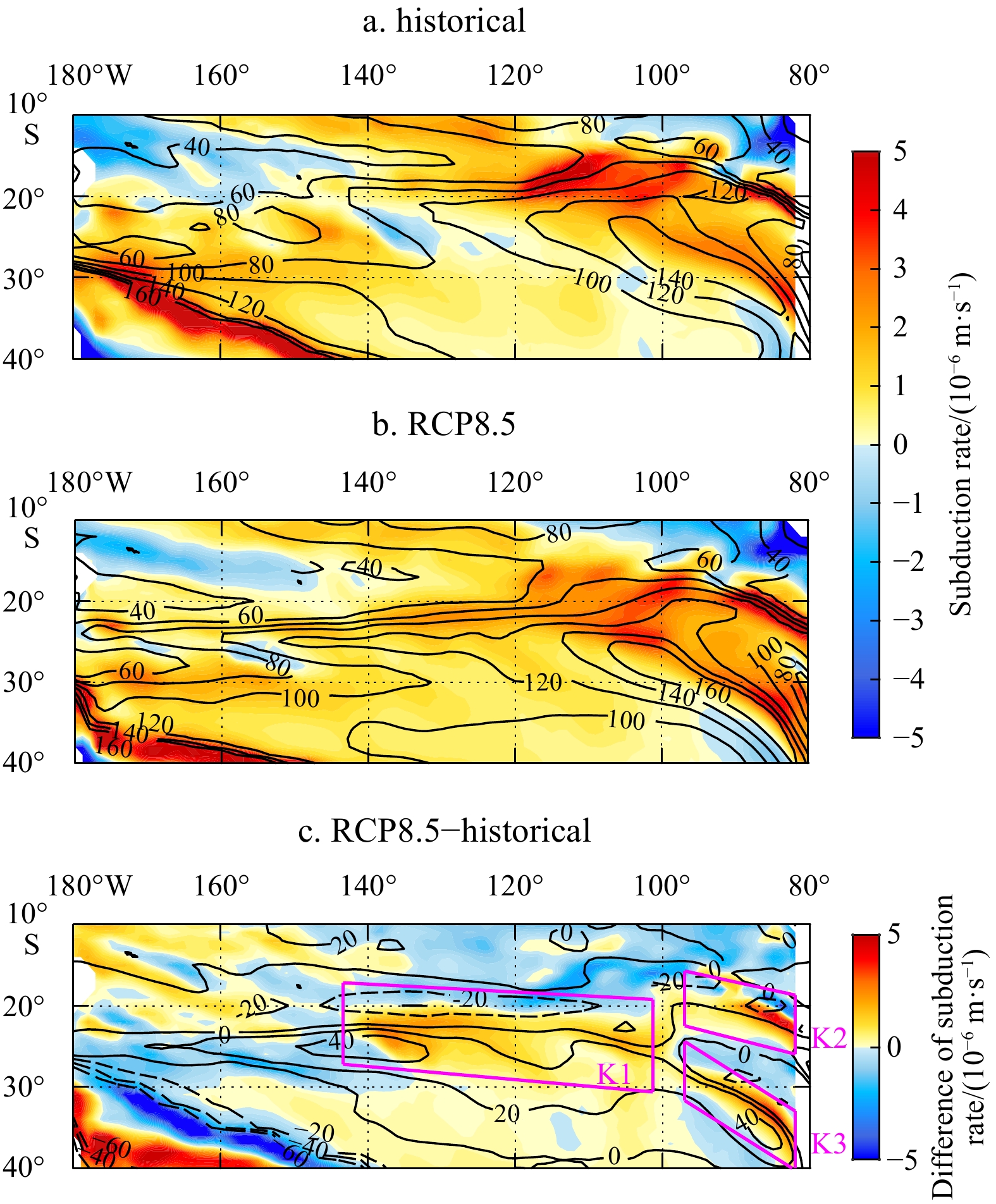
Three MLD fronts generate in the SEP highly dependent on the MLD non-uniform spatial pattern mentioned above. They are located in three regions: (1) K1, the north side of the “deep MLD tongue”; (2) K2, the northeast of the MLD maximum region; and (3) K3, the south side of the weak “shallow tongue” near the east boundary (as shown in Fig. 3c). In previous studies, we have confirmed that the MLD front is the key factor of the subduction rate, and then influences the mode water formation in the northeast Pacific (Xia et al., 2018, 2021). In this paper, we check the subduction rate in this model and find a similar result. As shown in Fig. 3a, the subduction rate is almost positive in the whole basin, which indicates that water is subducted into the deep ocean widely in the subtropical South Pacific in September. But we could still confirm three maximum areas in the SEP and one maximum area in the subtropical Southwest Pacific. All of the subduction maximum regions are highly corresponding with the MLD fronts (the density of the black contours could represent the front intensity in Fig. 3). We still focus on the SEP region in this paper and discuss the MLD front change after global warming next.
Figure
3.
The mean mixed layer depth (MLD, contours, interval 20 m) and subduction rate (shading, positive means subduction) in September in historical simulation (a) and RCP8.5 experiment (b); and the differences of MLD (contours, interval: 20 m) and subduction rate (shading) between two scenarios (RCP 8.5 minus historical) (c). Magenta frames in c represent the three key regions where subduction increases significantly in the SEP, marked as K1, K2 and K3, respectively. In c, positive subduction rate means subduction increases.
3.2
MLD variability in a warmer climate and its influence on subduction change
RCP8.5 experiment has been used to represent an extremely warmer climate in the future in this paper. MLD deepens obviously in most of the chosen regions in the RCP8.5 scenario, and this phenomenon has been mentioned in previous research (Luo et al., 2011). We have shown the spatially non-uniform MLD pattern in the present climate above. While the MLD variability is also spatially dependent after global warming in this model (Fig. 3c). We will explore the detail in the next paragraph. As MLD front intensity dominants the subduction process, we check the subduction rate and the MLD front changes together.
Compared to the historical simulation, the subduction rate increases in basin-scale but significantly in the three key regions (marked as K1, K2 and K3 in Fig. 3c) after global warming. The increasing subduction would accelerate the mixed layer water intrusion into the permanent thermocline under this warmer climate. All the key regions are corresponding with the MLD changing fronts. For example, MLD deepens to the south of Region K1 (solid lines in Fig. 3c, where the MLD is relatively deep in historical simulation) and shallows to the north of Region K1 (dashed lines in Fig. 3c, where the MLD is quite shallow in historical simulation). As a result, the MLD front in Region K1 is strengthened and moves southward in the RCP8.5 experiment. There are similar changes in the other two regions. These variabilities in three key regions indicate that the MLD front is not only important under the present climate, but also one dominant factor on the subduction change after global warming. The process of how MLD influences the subduction rate has been described in detail in our previous studies (Xia et al., 2015, 2018).
In conclusion, the MLD is non-uniform in the present climate, while the MLD variation from historical simulation to RCP8.5 scenario experiment is also non-uniform in the SEP. The original shallow mixed layer shoals but the original deep MLD becomes deeper in all key regions, enhancing the MLD front and the subduction rate. It could better explain why more mode water formed under a warmer climate (Luo et al., 2011). The above change also impacts that the MLD front is generally more sensitive than the local MLD to climate variability, not only in the subtropical Northeast Pacific (Xia et al., 2018) but also in the SEP.
4.
The mechanisms of the MLD change after global warming
In Section 3, we described the MLD climatology patterns in the present climate and future warmer projection. MLD non-uniform variability in the future changes the MLD front location and intensity, and then influences the subduction variability. Especially, the most visible changes locate in the three key regions, which indicate the MLD and its front changes are locally and non-uniform. Corresponding to the deepening of the mixed layer, the major dominant factors will be discussed in this section, including Ekman pumping caused by the wind stress, net heat flux, freshwater flux, and the ocean advection.
4.1
Ekman pumping and buoyancy flux
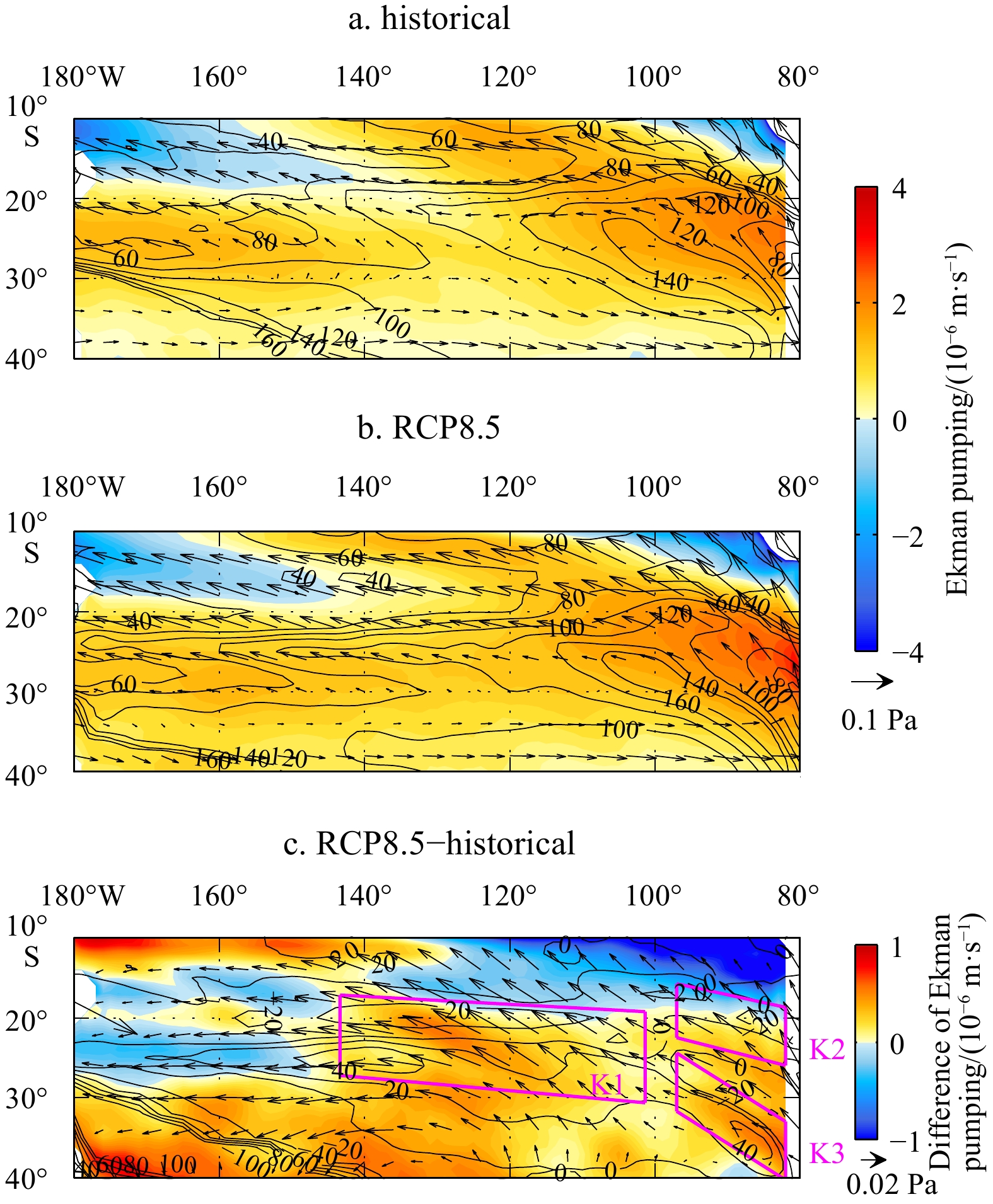
As shown in Fig. 4a, the model could simulate the southeast trade wind near the equator and a westerly jet in the middle latitudes in the subtropical South Pacific. There is positive (downwards) Ekman pumping in almost the whole basin, and larger absolute values of positive Ekman pumping are located in the west and east of the subtropical South Pacific (about 25°S) respectively, generally consistent with the two MLD local maximum regions (contours in Fig. 4, over 120 m in the west and 100 m in the east). However, the Ekman pumping maximum core in the SEP (25°S, 85°W) locates to the north of the MLD maximum core (>140 m), which implies that the Ekman pumping could not fully explain the MLD maximum formation. Considering the upwelling near the west coast of South America (cold colors in Fig. 4a), the Ekman pumping is the major factor determining the northeastern boundary of the MLD maximum region (similar to Huang, 2010). This result is also highly consistent with the observation from Quick Scatterometer winds (Liu and Lu, 2016). After global warming, the trade wind (north of 30°S) is increased (Fig. 4c) and enhances the downward Ekman pumping to the south of 19°S, except for the west of 150°W. This Ekman pumping variability helps to deepen the MLD in almost the whole basin, but not consistent with the actual non-uniform MLD change pattern (contours in Fig. 4). For example, the MLD deepens in the south of Region K1 but shoals in the north, but downward Ekman pumping increases in all of Region K1. However, the Ekman pumping variability contributes to the MLD change in Region K2 well. This phenomenon indicates that the contribution of Ekman pumping variability is regionally varying and only dominant in Region K2 after global warming in this model (Table 1, red arrows means positive effect for the corresponding MLD change).
Figure
4.
The mean mixed layer depth (MLD, contours, interval 20 m), wind stress (vectors), and Ekman pumping (shading, downward is positive, contribute to deepening the MLD) in September in historical simulation (a) and RCP8.5 experiment (b); and the differences of wind stress (vectors) and Ekman pumping (shading) between two scenarios (RCP 8.5 minus historical) (c). Magenta frames in c represent the three key regions defined in Fig. 3. In a and b, positive subduction rate means subduction, and in c, postive Ekman pumping means the downward Ekman pumping increases.
Table
1.
Qualitative comparison of the contributions of major factors to the MLD change after global warming
Variable
Region K1
Region K2
Region K3
North
South
North
South
North
South
ΔMLD
↓
↑
↓
↑
↓
↑
$ \Delta {w}_{\mathrm{e}} $
↑
↑
↓
↑
↑
↑
ΔQ
↓
↑
↓
↓
↑
↓
Δ(E−P)
↑
↑
↑
↑
↑
↑
ΔPDHA
↑
↑
↑
↓
↓
↑
ΔPDHAg
↓
↓
↓
↓
↓
↓
ΔPDHAe
↑
↑
↑
↓
↑
↑
Note: Regions K1, K2 and K3 are the three key regions defined in Fig. 3c. ΔMLD, $ {\Delta w}_{\mathrm{e}} $, ΔQ, Δ(E−P), ΔPDHA represent the changes of mixed layer depth, Ekman pumping (positive values help the MLD deepening), net heat flux from the atmosphere to the ocean (positive values help the MLD shoaling), freshwater flux (evaporation minus precipitation, positive helps the MLD deepening) and upper—ocean potential—density horizontal advection (positive helps the MLD shoaling) after global warming, respectively. $ \Delta {\mathrm{P}\mathrm{D}\mathrm{H}\mathrm{A}}_{\mathrm{e}} $ and $ {\Delta \mathrm{P}\mathrm{D}\mathrm{H}\mathrm{A}}_{\mathrm{g}} $ are the two components of $ \Delta $PDHA: Ekman advection and geostrophic advection change. ↑ means the factor increases after global warming, while ↓ means the factor decreases; the red color represents that factor provides a positive contribution to the regional MLD change.
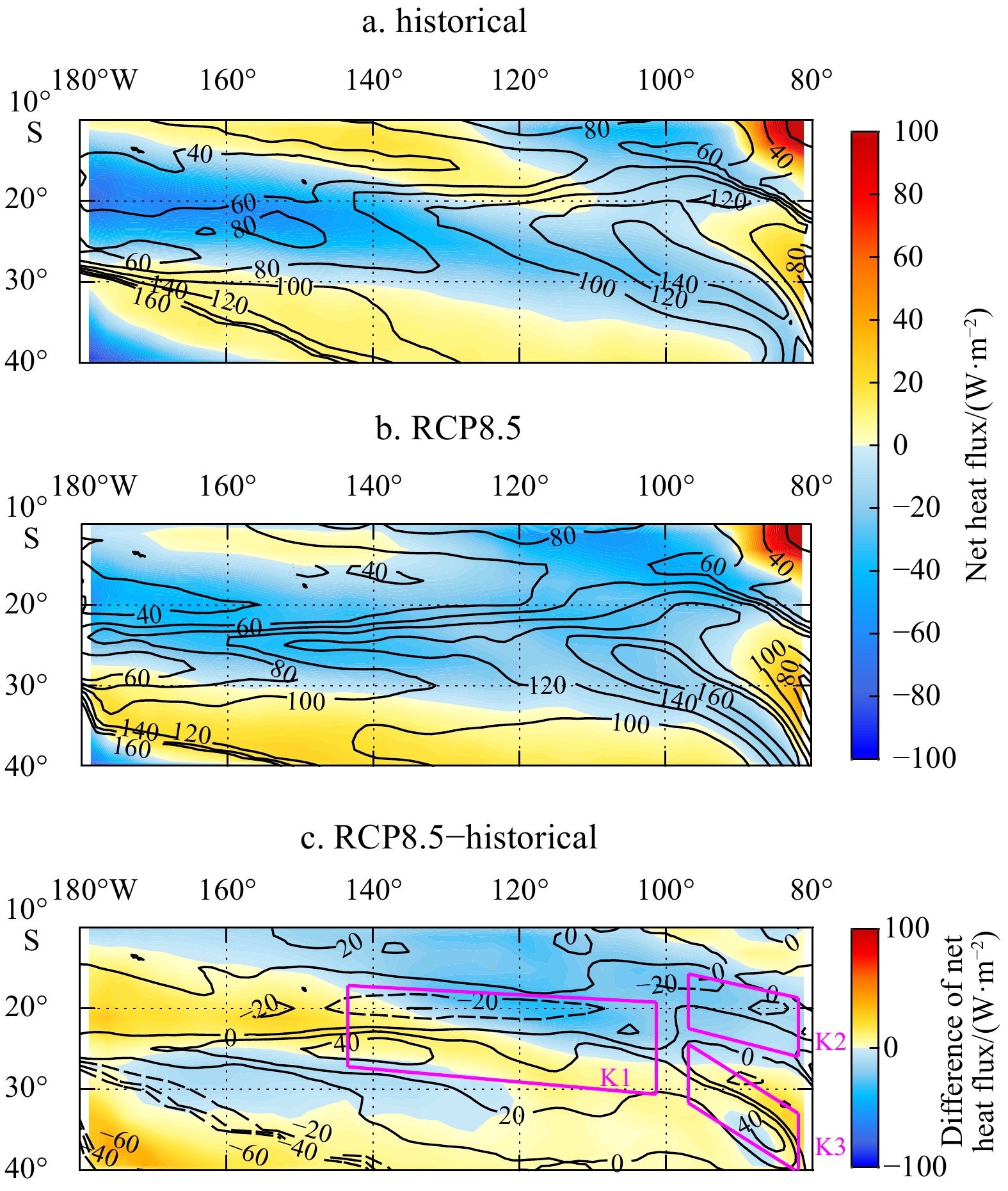
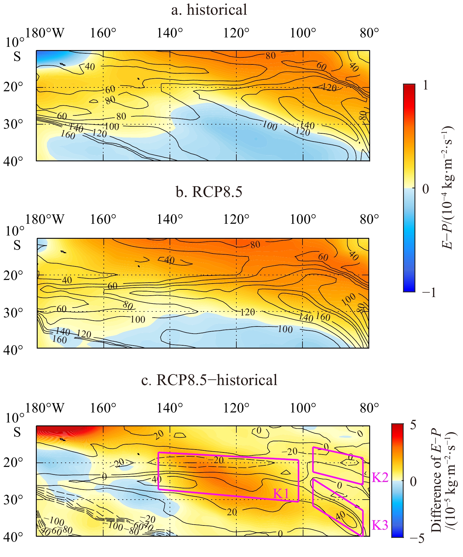
Including the heat flux and freshwater flux, buoyancy flux is also important for the MLD deepening in austral winter. We calculate the net heat flux from the atmosphere to the ocean in Fig. 5. The spatial pattern of heat flux in the RCP8.5 scenario (Fig. 5b) is similar to that in the historical simulation (Fig. 5a). Here the negative values mean the ocean loses heat to the atmosphere and contributes to deepening the MLD. Similar to heat flux, we show the freshwater flux in Fig. 6. The positive values mean evaporation larger than precipitation, increasing the vertical mixing process and deepening the MLD. No matter in which experiment, both heat flux and freshwater flux are quite significant for the MLD deepening. However, if we check the difference (RCP8.5 minus historical), we were surprised to find that both heat flux and freshwater flux changes are not consistent with the MLD change. For example, negative values in the north of the region K1 (Fig. 5c, north of 25°S, east of 130°W) represent ocean loses more heat and contributes to deepening the MLD, while the MLD decreases actually in this region. A similar result occurs in the south of Region K1. Generally, the heat flux variability makes positive contributions to the MLD change only in Region K3 (Fig. 5c). The freshwater flux is strengthened almost in the whole basin, regardless of whether MLD is deepened or shallowed (Fig. 6c).
Figure
5.
The mean mixed layer depth (MLD, contours, interval 20 m) and net heat flux from the atmosphere to ocean (shading) in September in historical simulation (a) and RCP8.5 experiment (b); and the differences of MLD and net heat flux (shading, unit: W/m2) between two scenarios (RCP 8.5 minus historical) (c). Magenta frames in c represent the three regions defined in Fig. 3. In a and b, positive net heat flux means ocean get heat and helps to shallow the MLD, and in c positive difference of netheat flux means ocean get more heat.
Figure
6.
The mean mixed layer depth (MLD, contours, interval 20 m) and E−P flux (evaporation minus precipitation) from the atmosphere to ocean (shading) in September in historical simulation (a) and RCP8.5 experiment (b); and the differences of MLD and E−P flux (shading) between two scenarios (RCP 8.5 minus historical) (c). Magenta frames in c represent the three regions defined in Fig. 3. In a and b, positive E−P flux means the upper ocean salinity increasing and helps to deepen the MLD, and in c, positive difference of E−P flux means ocean becomes saltier.
In other words, Ekman pumping, heat flux and freshwater flux are all important for the MLD spatial pattern in both historical and RCP8.5 scenarios, but none of them could explain the MLD non-uniform change clearly. So ocean advection will be considered in the next part in detail.
4.2
Potential density horizontal advection
As shown in Section 4.1, both heat flux and freshwater flux affect the vertical mixing process obviously in this region, we could not only analyze the ocean heat variability, as we did in some previous research (Xia et al., 2015, 2021). Combined with the temperature and salinity advection effect, the role of potential-density horizontal advection (PDHA) in the upper ocean is investigated in this section. PDHA has been defined in Section 2.2.
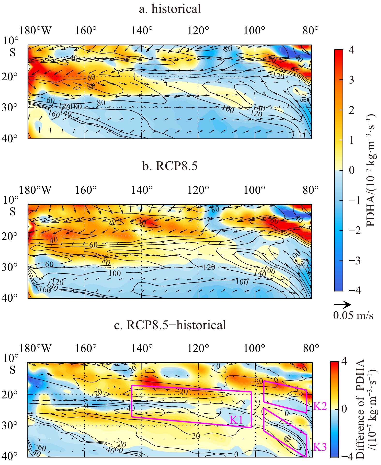
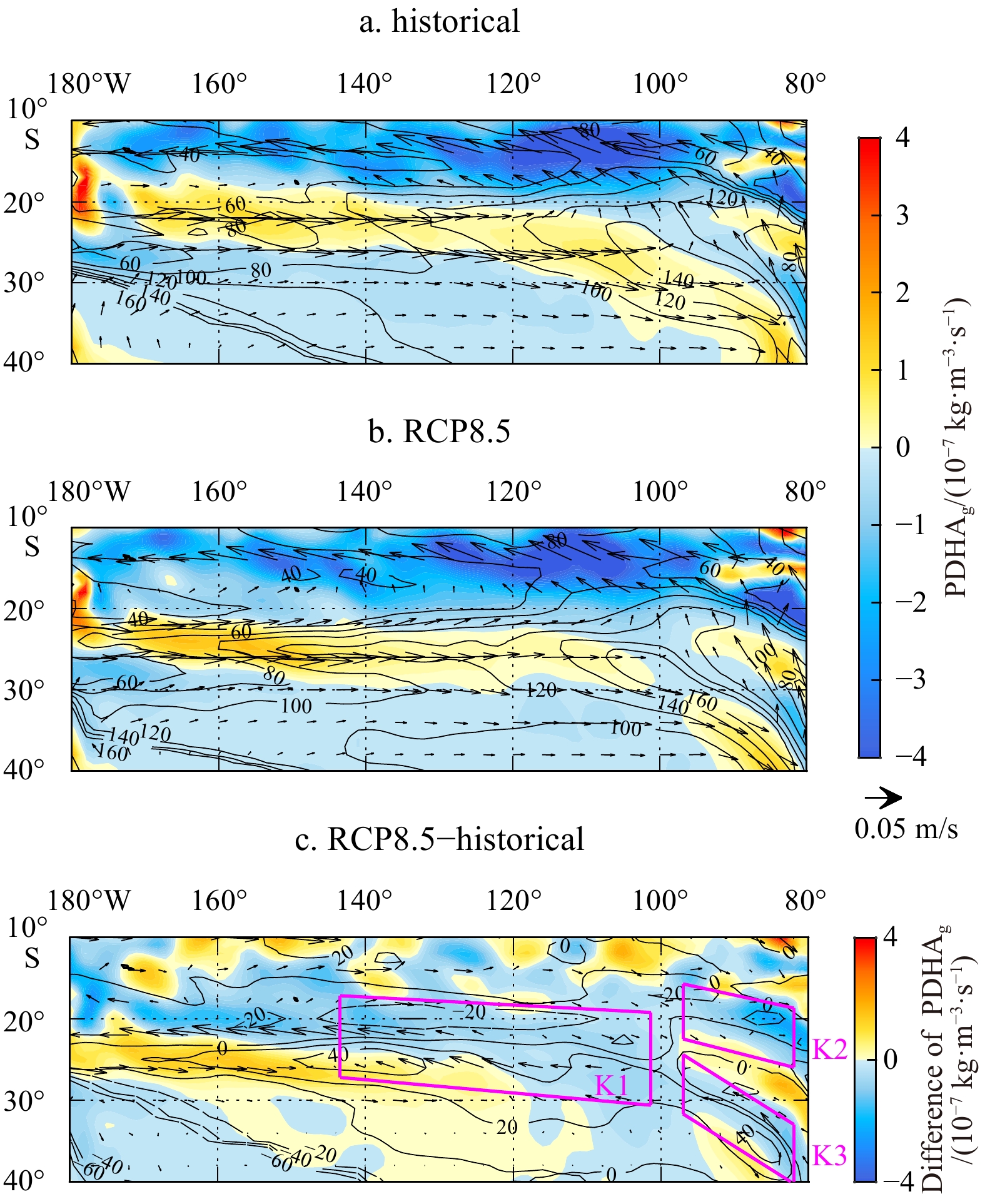
In the historical simulation, we find a large PDHA “positive tongue” (about 23−28°S) extends far to the east, corresponding to the MLD “shallow tongue” near Region K1 (Fig. 7a). The formation of PDHA “positive tongue” seems based on the geostrophic advection by STCC (Fig. 8a), by transporting lighter water in the upper layer and stabilizing the stratification (Liu and Lu, 2016). The STCC blocks the westward extension of the deep mixed layer and forms the MLD “shallow tongue”, then combines the westward advection to the north side and causes the opposite PDHA “negative tongue” (about 18°–23°S) to the north side. These two PDHA “tongues” are highly consistent with the two MLD “tongues”. Due to the lack of ocean velocity data, the previous research could only explain the advection effect by geostrophic velocity. To verify this, we compare the Ekman and geostrophic components ($ {\mathrm{P}\mathrm{D}\mathrm{H}\mathrm{A}}_{\mathrm{e}} $ and $ {\mathrm{P}\mathrm{D}\mathrm{H}\mathrm{A}}_{\mathrm{g}} $) next. It is easy to find a strong eastward $ {\mathrm{P}\mathrm{D}\mathrm{H}\mathrm{A}}_{\mathrm{g}} $ in both Figs 8a and b, extending over 100°W between 20°S and 30°S. While the strength and north-south range of the $ {\mathrm{P}\mathrm{D}\mathrm{H}\mathrm{A}}_{\mathrm{g}} $ “positive tongue” is smaller to the west of 135°W but larger to the east of 135°W than that of total PDHA, which implies that the $ {\mathrm{P}\mathrm{D}\mathrm{H}\mathrm{A}}_{\mathrm{e}} $ component caused by wind stress provide a similar contribution with $ {\mathrm{P}\mathrm{D}\mathrm{H}\mathrm{A}}_{\mathrm{g}} $ to the west of 135°W but an opposite contribution to the east of 135°W. The contribution of $ {\mathrm{P}\mathrm{D}\mathrm{H}\mathrm{A}}_{\mathrm{e}} $ component could also be confirmed in Fig. 9a directly. In other words, the MLD “shallow tongue” and “deep tongue” in Region K1 are the combined effects of two PDHA components in the present climate. The changes of both components may be the sources for the amplified indented structure of MLD in this model.
Figure
7.
The mean mixed layer depth (MLD, contours, interval 20 m), the vertical average velocity (vectors), and the PDHA (shading, vertical integration above 100 m, positive values help MLD shoals) in September in historical simulation (a) and RCP8.5 experiment (b); and the differences of MLD, the vertical average velocity, and the PDHA (shading) between two scenarios (RCP 8.5 minus historical) (c). Magenta frames in c represent the three regions defined in Fig. 3.
Figure
8.
The mean mixed layer depth (MLD, contours, interval 20 m), the vertical average geostrophic velocity (vectors) and the $ {\mathrm{P}\mathrm{D}\mathrm{H}\mathrm{A}}_{\mathrm{g}} $ (shading, vertical integration above 100 m, positive values help MLD shoals) in September in historical simulation (a) and RCP8.5 experiment (b); and the differences of MLD, the vertical average geostrophic velocity and the $ {\mathrm{P}\mathrm{D}\mathrm{H}\mathrm{A}}_{\mathrm{g}} $ (shading) between two scenarios (RCP 8.5 minus historical) (c). Magenta frames in c represent the three regions defined in Fig. 3.
Figure
9.
The mean mixed layer depth (MLD, contours, interval 20 m), the vertical average Ekman horizontal velocity (vectors) and the $ {\mathrm{P}\mathrm{D}\mathrm{H}\mathrm{A}}_{\mathrm{e}} $ (shading, vertical integration above 100 m, positive values help MLD shoals) in September in historical simulation (a) and RCP8.5 experiment (b); and the differences of MLD, the vertical average Ekman horizontal velocity and the $ {\mathrm{P}\mathrm{D}\mathrm{H}\mathrm{A}}_{\mathrm{e}} $ (shading) between two scenarios (RCP 8.5 minus historical) (c). Magenta frames in c represent the three regions defined in Fig. 3.
In the present climate, the total PDHA also explains the north boundary of MLD maximum near Region K2 well, as a strong positive PDHA limits the MLD deepening (Fig. 7a). Comparing its two components (Figs 8a and 9a), we find a strong positive $ {\mathrm{P}\mathrm{D}\mathrm{H}\mathrm{A}}_{\mathrm{e}} $ is consistent with the PDHA, while the $ {\mathrm{P}\mathrm{D}\mathrm{H}\mathrm{A}}_{\mathrm{g}} $ is negative in Region K2. Considering other factors, we conclude that the $ {\mathrm{P}\mathrm{D}\mathrm{H}\mathrm{A}}_{\mathrm{e}} $ and the Ekman pumping are most dominant for the MLD pattern in Region K2, both affected by surface wind stress. But the contribution of PDHA is not quite significant in Region K3, where heat flux is more important.
The PDHA vertical structure is shown clearly in different regions in Fig. 10. In the present climate, the shallow MLD (north of 18°S) is consistent with the high positive PDHA upper 50 meters and a weak negative PDHA under the mixed layer (Fig. 10a and Fig. 10c). This indicates that the Ekman component is dominant in the north of 18°S. By contrast, a weak negative PDHA (vertical integration) occurs near the MLD “deep tongue” (18°–23°S), contributing to the deepening MLD. Notice that another positive PDHA affects the MLD “shallow tongue” (23°–28°S), but deeper than that north of 18°S.
Figure
10.
Depth-latitude section of PDHA (shading) along 140°W to 130°W (a, b) and along 87°W to 85°W (c, d). a and c. the present climate, and b and d. The change after global warming (RCP8.5 minus historical). Superimposed are the MLD in historical (black lines) and RCP8.5 (dashed lines). We check the PDHA in Region K1 from a and b, and Regions K2 and K3 from c and d.
After global warming, we find the variability of PDHA spatial pattern is more non-uniform than the changes of Ekman pumping and buoyancy flux. For example, the significantly increased PDHA (north of 21°S, 150°−110°W) is highly consistent with the local MLD shallowing in the north of Region K1 (Fig. 7c). On the contrary, the PDHA is a little decreased on the south side, deepening the MLD. In other words, the strengthened MLD front in Region K1 is generally caused by the antisymmetric change of PDHA on both sides of the front. The depth-latitude section of the PDHA (Fig. 10b) also shows this consistency. The increased positive PDHA near (21°−15°S) concentrates on upper 50 meters, which implies the increased PDHA is due to the strengthened $ {\mathrm{P}\mathrm{D}\mathrm{H}\mathrm{A}}_{\mathrm{e}} $ (also seen in Fig. 9c). While the decreased PDHA south of 22°S seems to source from the $ {\mathrm{P}\mathrm{D}\mathrm{H}\mathrm{A}}_{\mathrm{g}} $ change. Besides, the increased positive PDHA occurs a significant southward displacement, leading to the southward MLD front.
Especially, we find the STCC increases to the west of 135°W and provides lighter water, but decreases to the east of 135°W. As a result, the source of decreased PDHA in the south of Region K1 is more complex, resulting from $ {\mathrm{P}\mathrm{D}\mathrm{H}\mathrm{A}}_{\mathrm{e}} $ west of 135°W (Fig. 9c) but $ {\mathrm{P}\mathrm{D}\mathrm{H}\mathrm{A}}_{\mathrm{g}} $ east of 135°W (Fig. 8c). A similar analysis shows that the PDHA change also works in Region K2, but not significant in Region K3 (Figs 7c, 8c, 9c and 10d). We summarize the PDHA change contributions with other factors in Table 1.
In summary, the PDHA, including the Ekman and geostrophic components, is important for both the MLD climatology non-uniform pattern and its non-uniform change after global warming. Comparing with Ekman pumping and buoyancy flux, we find these factors are regionally dependent seriously. We summarize the contributions of the above elements to the three key regions of MLD change in Table 1. One important fact is that many factors contribute to the MLD deepening in the south of the three key regions, but only one or two factors making positive contributions to the MLD shoaling in the north sides. In Region K1, the increased $ {\mathrm{P}\mathrm{D}\mathrm{H}\mathrm{A}}_{\mathrm{e}} $ is dominant for the MLD shoaling in the north side after global warming. The MLD shoaling in the north of Region K2 is mainly due to the changes of $ {\mathrm{P}\mathrm{D}\mathrm{H}\mathrm{A}}_{\mathrm{e}} $ and Ekman pumping, which implies the wind stress is the most significant factor. While net heat flux seems more important in Region K3, leading to the weak MLD “shallow tongue” in the present climate and the corresponding variability after global warming. Finally, the southward MLD front seems mainly due to the significant southward displacement of PDHA in all the key regions.
5.
Conclusions and discussion
A qualitative investigation of the relative importance of Ekman pumping, net surface heat flux, freshwater flux, and horizontal density advection on the winter MLD in the subtropical Southeast Pacific was conducted in this study using the ESM2M in both historical simulation and RCP8.5 scenario. Similar to previous research, the seasonal MLD is deepened from May and reaches its maximum in September in this model. A local MLD maximum (>160 m) exists near (24°S, 104°W) in the historical simulation. The MLD spatial pattern is non-uniform in the present climate, with three significant characteristics: (1) MLD maximum region extends from the Southeast Pacific to the West Pacific and forms a “deep tongue” until 135°W, influenced by an obviously “shallow tongue” of MLD extending eastward; (2) the northern boundary of the MLD maximum is smoothly and almost zonally near 18°S, and shallows sharply to the northeast; and (3) there is a relatively shallow MLD inserted into the eastern boundary near (26°S, 80°W) as a weak “shallow tongue”. Therefore, three MLD fronts generate due to the MLD non-uniform spatial pattern, located in the three key regions: (1) K1, the north side of the “deep MLD tongue”; (2) K2, the northeast of the MLD maximum region; and (3) K3, the south side of the weak “shallow tongue” near the east boundary (Fig. 3c). The MLD fronts are highly corresponding with the large effective subduction rate.
The RCP8.5 experiment has been used to represent an extremely warmer climate in the future in this paper. From the RCP8.5 experiment, we find the MLD deepens or shallows spatially dependent after global warming (Fig. 3c), instead of uniformly deepening in this region. The MLD change influences the MLD front and then increases the subduction rate in the three key regions, consistent with the MLD three characteristics mentioned above. This distribution indicates that the MLD front is not only important under the present climate, but its change is also the dominant factor in the subduction variability after global warming. The MLD front seems generally more sensitive than the local MLD to climate variability, not only in the subtropical Northeast Pacific (Xia et al., 2018) but also in the subtropical Northeast Pacific. The original shallow mixed layer shoals but the original deep MLD becomes deeper in all the key regions, enhancing the MLD front and the subduction rate.
Though similar MLD changes appear in these key regions, their dominant mechanisms are quite regionally varying. Comparing PDHA with Ekman pumping and buoyancy flux, we find the regional diversity of these factors are significant. As we summarized in Section 4, the MLD antisymmetric changes mainly source from the MLD shoaling in the north sides of the three regions, with dominant factors: $ {\mathrm{P}\mathrm{D}\mathrm{H}\mathrm{A}}_{\mathrm{e}} $ change for Region K1, $ {\mathrm{P}\mathrm{D}\mathrm{H}\mathrm{A}}_{\mathrm{e}} $ and Ekman pumping change for Region K2 and net heat flux change for Region K3. Thus, the contributions of all the factors are effective regionally and changing with the climate variability. Notice that the freshwater flux helps to deepen the MLD, but its distribution is more uniform in the whole basin, so it hardly works on the regional varying MLD. Table 1 also indicates that the PDHA, especially its Ekman component, is truly important for the MLD non-uniform variability after global warming. Though $ {\mathrm{P}\mathrm{D}\mathrm{H}\mathrm{A}}_{\mathrm{g}} $ controls the formation of the MLD “shallow tongue” (similar to Liu and Lu (2016)), its effects in three key regions are almost negative. Finally, the southward movement of the MLD front seems to be from the significant southward displacement of PDHA in all the key regions.
The spatial and temporal distributions and variations of the winter MLD control the MLD front, influencing the subduction process and the mode water formation. Considered about the important climate effects on the tropic region (Gu and Philander, 1997), a more accurate quantitative diagnostic on the MLD and subduction process is necessary for further work. For example, the Liang-Kleeman information flow method (Liang, 2014) may be one useful method for this multi-source forcing effects analysis (Jiang et al., 2019). Besides, we may also learn more about the inter mechanisms through multi-model comparison (Xia et al., 2018, 2021).
In recent years, more and more studies focus on the mesoscale eddy effect on the subduction process and the mode water formation. It is found that eddy activities contribute to the MLD variation in various time scales (days to years), and then impact the subduction process in many regions (Wen et al., 2020; Xu et al., 2016, 2017). As the CMIP5 models are generally in 1°$ \times $1° resolution, their output results could not resolve the eddy effect. With the development of high-resolution models in CMIP6, exploring the mesoscale eddies in decadal to multi-annual cycles in a warmer or colder climate becomes realizable, which will be carried out in our future research.
Acknowledgements
We appreciate all the observational and model reanalysis data provided by the Asia-Pacific Data Research Center, and we also thank the NOAA GFDL’s working group on coupled modeling for the ESM2M output.
Carton J A, Giese B S. 2008. A reanalysis of ocean climate using Simple Ocean Data Assimilation (SODA). Monthly Weather Review, 136(8): 2999–3017. doi: 10.1175/2007MWR1978.1
[2]
de Boyer Montégut C, Madec G, Fischer A S, et al. 2004. Mixed layer depth over the global ocean: an examination of profile data and a profile-based climatology. Journal of Geophysical Research: Oceans, 109(C12): C12003. doi: 10.1029/2004JC002378
[3]
Dong Shenfu, Sprintall J, Gille S T, et al. 2008. Southern ocean mixed-layer depth from Argo float profiles. Journal of Geophysical Research: Oceans, 113(C6): C06013
[4]
Dunne J P, John J G, Adcroft A J, et al. 2012. GFDL’s ESM2 global coupled climate-carbon earth system models: Part I. Physical formulation and baseline simulation characteristics. Journal of Climate, 25(19): 6646–6665. doi: 10.1175/JCLI-D-11-00560.1
[5]
Gu Daifang, Philander S G H. 1997. Interdecadal climate fluctuations that depend on exchanges between the tropics and extratropics. Science, 275(5301): 805–807. doi: 10.1126/science.275.5301.805
[6]
Hu Haibo, Liu Qinyu, Zhang Yuan, et al. 2011. Variability of subduction rates of the subtropical North Pacific mode waters. Chinese Journal of Oceanology and Limnology, 29(5): 1131–1141. doi: 10.1007/s00343-011-0237-x
[7]
Huang R X. 2010. Oceanic Circulation: Wind-driven and Thermohaline Processes. Cambridge, UK: Cambridge University Press, 360–369
[8]
Jiang Shunyu, Hu Haibo, Zhang Ning, et al. 2019. Multi-source forcing effects analysis using Liang-Kleeman information flow method and the community atmosphere model (CAM4.0). Climate Dynamics, 53(9): 6035–6053
[9]
Kara A B, Rochford P A, Hurlburt H E. 2003. Mixed layer depth variability over the global ocean. Journal of Geophysical Research: Oceans, 108(C3): 3079. doi: 10.1029/2000JC000736
[10]
Kraus E B. 1972. Atmospheric–Ocean Interaction. London: Oxford University Press, 255
[11]
Liang Xiangsan. 2014. Unraveling the cause-effect relation between time series. Physical Review E, 90(5): 052150. doi: 10.1103/PhysRevE.90.052150
[12]
Liu Qinyu, Lu Yiqun. 2016. Role of horizontal density advection in seasonal deepening of the mixed layer in the subtropical Southeast Pacific. Advances in Atmospheric Sciences, 33(4): 442–451. doi: 10.1007/s00376-015-5111-x
[13]
Liu Chengyan, Wang Zhaomin. 2014. On the response of the global subduction rate to global warming in coupled climate models. Advances in Atmospheric Sciences, 31(1): 211–218. doi: 10.1007/s00376-013-2323-9
[14]
Luo Yiyong, Liu Qinyu, Rothstein L M. 2009. Simulated response of North Pacific Mode Waters to global warming. Geophysical Re- search Letters, 36(23): L23609
[15]
Luo Yiyong, Liu Qinyu, Rothstein L M. 2011. Increase of South Pacific eastern subtropical mode water under global warming. Geophysical Research Letters, 38(1): L01601
[16]
Pond S, Pickard G L. 1983. Introductory Dynamical Oceanography. 2nd ed. New York: Pergamon, 379
[17]
Qiu Bo, Huang Ruixin. 1995. Ventilation of the North Atlantic and North Pacific: subduction versus obduction. Journal of Physical Oceanography, 25(10): 2374–2390. doi: 10.1175/1520-0485(1995)025<2374:VOTNAA>2.0.CO;2
[18]
Sato K, Suga T. 2009. Structure and modification of the south pacific eastern subtropical mode water. Journal of Physical Oceanography, 39(7): 1700–1714. doi: 10.1175/2008JPO3940.1
[19]
Sprintall J, Tomczak M. 1992. Evidence of the barrier layer in the surface layer of the tropics. Journal of Geophysical Research: Oceans, 97(C5): 7305–7316. doi: 10.1029/92JC00407
[20]
Taylor K E, Stouffer R J, Meehl G A. 2012. An overview of CMIP5 and the experiment design. Bulletin of the American Meteorological Society, 93(4): 485–498. doi: 10.1175/BAMS-D-11-00094.1
[21]
Wang Yingying, Luo Yiyong. 2020. Variability of spice injection in the upper ocean of the southeastern Pacific during 1992–2016. Climate Dynamics, 54(5): 3185–3200
[22]
Wen Zhibin, Hu Haibo, Song Zhenya, et al. 2020. Different influences of mesoscale oceanic eddies on the North Pacific subsurface low potential vorticity water mass between winter and summer. Journal of Geophysical Research: Oceans, 125(1): e2019JC015333
[23]
Williams R G. 1991. The role of the mixed layer in setting the potential vorticity of the main thermocline. Journal of Physical Oceanography, 21(12): 1803–1814. doi: 10.1175/1520-0485(1991)021<1803:TROTML>2.0.CO;2
Xia Ruibin, Li Bingrui, Cheng Chen. 2021. Response of the mixed layer depth and subduction rate in the subtropical Northeast Pacific to global warming. Acta Oceanologica Sinica, 40(4): 1–9. doi: 10.1007/s13131-021-1818-y
[26]
Xia Ruibin, Liu Chengyan, Cheng Chen. 2018. On the subtropical Northeast Pacific mixed layer depth and its influence on the subduction. Acta Oceanologica Sinica, 37(3): 51–62. doi: 10.1007/s13131-017-1102-3
[27]
Xia Ruibin, Liu Qinyu, Xu Lixiao, et al. 2015. North Pacific Eastern Subtropical mode water simulation and future projection. Acta Oceanologica Sinica, 34(3): 25–30. doi: 10.1007/s13131-015-0630-y
[28]
Xie S-P, Du Yan, Huang Gang, et al. 2010. Decadal shift in El Niño influences on Indo-western Pacific and East Asian climate in the 1970 s. Journal of Climate, 23(12): 3352–3368. https://doi.org/10.1175/2010JCLI3429.1
[29]
Xu Lixiao, Li Peiliang, Xie Shangping, et al. 2016. Observing mesoscale eddy effects on mode-water subduction and transport in the North Pacific. Nature Communications, 7(1): 10505. doi: 10.1038/ncomms10505
[30]
Xu Lixiao, Xie S-P, Liu Qinyu, et al. 2017. Evolution of the North Pacific subtropical mode water in anticyclonic eddies. Journal of Geophysical Research:Oceans, 122(12): 10118–10130. doi: 10.1002/2017JC013450
Ping Yang, Fuchang Yu, Jing Liu, et al. Multivariate VAR System of Regional Economic Growth under Big Data. Heliyon, 2024. doi:10.1016/j.heliyon.2024.e38517
Ruibin Xia, Yijun He, Tingting Yang. Simulation and future projection of the mixed layer depth and subduction process in the subtropical Southeast Pacific[J]. Acta Oceanologica Sinica, 2021, 40(12): 104-113. doi: 10.1007/s13131-021-1877-0
Ruibin Xia, Yijun He, Tingting Yang. Simulation and future projection of the mixed layer depth and subduction process in the subtropical Southeast Pacific[J]. Acta Oceanologica Sinica, 2021, 40(12): 104-113. doi: 10.1007/s13131-021-1877-0
Table
1.
Qualitative comparison of the contributions of major factors to the MLD change after global warming
Variable
Region K1
Region K2
Region K3
North
South
North
South
North
South
ΔMLD
↓
↑
↓
↑
↓
↑
$ \Delta {w}_{\mathrm{e}} $
↑
↑
↓
↑
↑
↑
ΔQ
↓
↑
↓
↓
↑
↓
Δ(E−P)
↑
↑
↑
↑
↑
↑
ΔPDHA
↑
↑
↑
↓
↓
↑
ΔPDHAg
↓
↓
↓
↓
↓
↓
ΔPDHAe
↑
↑
↑
↓
↑
↑
Note: Regions K1, K2 and K3 are the three key regions defined in Fig. 3c. ΔMLD, $ {\Delta w}_{\mathrm{e}} $, ΔQ, Δ(E−P), ΔPDHA represent the changes of mixed layer depth, Ekman pumping (positive values help the MLD deepening), net heat flux from the atmosphere to the ocean (positive values help the MLD shoaling), freshwater flux (evaporation minus precipitation, positive helps the MLD deepening) and upper—ocean potential—density horizontal advection (positive helps the MLD shoaling) after global warming, respectively. $ \Delta {\mathrm{P}\mathrm{D}\mathrm{H}\mathrm{A}}_{\mathrm{e}} $ and $ {\Delta \mathrm{P}\mathrm{D}\mathrm{H}\mathrm{A}}_{\mathrm{g}} $ are the two components of $ \Delta $PDHA: Ekman advection and geostrophic advection change. ↑ means the factor increases after global warming, while ↓ means the factor decreases; the red color represents that factor provides a positive contribution to the regional MLD change.
Note: Regions K1, K2 and K3 are the three key regions defined in Fig. 3c. ΔMLD, $ {\Delta w}_{\mathrm{e}} $, ΔQ, Δ(E−P), ΔPDHA represent the changes of mixed layer depth, Ekman pumping (positive values help the MLD deepening), net heat flux from the atmosphere to the ocean (positive values help the MLD shoaling), freshwater flux (evaporation minus precipitation, positive helps the MLD deepening) and upper—ocean potential—density horizontal advection (positive helps the MLD shoaling) after global warming, respectively. $ \Delta {\mathrm{P}\mathrm{D}\mathrm{H}\mathrm{A}}_{\mathrm{e}} $ and $ {\Delta \mathrm{P}\mathrm{D}\mathrm{H}\mathrm{A}}_{\mathrm{g}} $ are the two components of $ \Delta $PDHA: Ekman advection and geostrophic advection change. ↑ means the factor increases after global warming, while ↓ means the factor decreases; the red color represents that factor provides a positive contribution to the regional MLD change.
Figure 1. The September mean mixed layer depth (MLD, shading) based on Argo (a), SODA (b), ECCO2 (c), and GFDL-ESM2M (d–f, with different MLD definition). The MLD in a–d is defined by $ \Delta \rho =0.1 $ kg/m3, and the MLD in e and f are defined by $\Delta \rho=0.125 $ kg/m3 and $\Delta T=0.5 $ °C, respectively. The bold black contours (100 m MLD) represent the MLD front roughly.
Figure 2. Monthly mean mixed layer depth (MLD, shading) in May (a, g), June (b, h), July (c, i), August (d, j), September (e, k), and October (f, l) based on Argo (a–f), and GFDL-ESM2M (g–l). The bold black contours (100 m MLD) represent the MLD front roughly.
Figure 3. The mean mixed layer depth (MLD, contours, interval 20 m) and subduction rate (shading, positive means subduction) in September in historical simulation (a) and RCP8.5 experiment (b); and the differences of MLD (contours, interval: 20 m) and subduction rate (shading) between two scenarios (RCP 8.5 minus historical) (c). Magenta frames in c represent the three key regions where subduction increases significantly in the SEP, marked as K1, K2 and K3, respectively. In c, positive subduction rate means subduction increases.
Figure 4. The mean mixed layer depth (MLD, contours, interval 20 m), wind stress (vectors), and Ekman pumping (shading, downward is positive, contribute to deepening the MLD) in September in historical simulation (a) and RCP8.5 experiment (b); and the differences of wind stress (vectors) and Ekman pumping (shading) between two scenarios (RCP 8.5 minus historical) (c). Magenta frames in c represent the three key regions defined in Fig. 3. In a and b, positive subduction rate means subduction, and in c, postive Ekman pumping means the downward Ekman pumping increases.
Figure 5. The mean mixed layer depth (MLD, contours, interval 20 m) and net heat flux from the atmosphere to ocean (shading) in September in historical simulation (a) and RCP8.5 experiment (b); and the differences of MLD and net heat flux (shading, unit: W/m2) between two scenarios (RCP 8.5 minus historical) (c). Magenta frames in c represent the three regions defined in Fig. 3. In a and b, positive net heat flux means ocean get heat and helps to shallow the MLD, and in c positive difference of netheat flux means ocean get more heat.
Figure 6. The mean mixed layer depth (MLD, contours, interval 20 m) and E−P flux (evaporation minus precipitation) from the atmosphere to ocean (shading) in September in historical simulation (a) and RCP8.5 experiment (b); and the differences of MLD and E−P flux (shading) between two scenarios (RCP 8.5 minus historical) (c). Magenta frames in c represent the three regions defined in Fig. 3. In a and b, positive E−P flux means the upper ocean salinity increasing and helps to deepen the MLD, and in c, positive difference of E−P flux means ocean becomes saltier.
Figure 7. The mean mixed layer depth (MLD, contours, interval 20 m), the vertical average velocity (vectors), and the PDHA (shading, vertical integration above 100 m, positive values help MLD shoals) in September in historical simulation (a) and RCP8.5 experiment (b); and the differences of MLD, the vertical average velocity, and the PDHA (shading) between two scenarios (RCP 8.5 minus historical) (c). Magenta frames in c represent the three regions defined in Fig. 3.
Figure 8. The mean mixed layer depth (MLD, contours, interval 20 m), the vertical average geostrophic velocity (vectors) and the $ {\mathrm{P}\mathrm{D}\mathrm{H}\mathrm{A}}_{\mathrm{g}} $ (shading, vertical integration above 100 m, positive values help MLD shoals) in September in historical simulation (a) and RCP8.5 experiment (b); and the differences of MLD, the vertical average geostrophic velocity and the $ {\mathrm{P}\mathrm{D}\mathrm{H}\mathrm{A}}_{\mathrm{g}} $ (shading) between two scenarios (RCP 8.5 minus historical) (c). Magenta frames in c represent the three regions defined in Fig. 3.
Figure 9. The mean mixed layer depth (MLD, contours, interval 20 m), the vertical average Ekman horizontal velocity (vectors) and the $ {\mathrm{P}\mathrm{D}\mathrm{H}\mathrm{A}}_{\mathrm{e}} $ (shading, vertical integration above 100 m, positive values help MLD shoals) in September in historical simulation (a) and RCP8.5 experiment (b); and the differences of MLD, the vertical average Ekman horizontal velocity and the $ {\mathrm{P}\mathrm{D}\mathrm{H}\mathrm{A}}_{\mathrm{e}} $ (shading) between two scenarios (RCP 8.5 minus historical) (c). Magenta frames in c represent the three regions defined in Fig. 3.
Figure 10. Depth-latitude section of PDHA (shading) along 140°W to 130°W (a, b) and along 87°W to 85°W (c, d). a and c. the present climate, and b and d. The change after global warming (RCP8.5 minus historical). Superimposed are the MLD in historical (black lines) and RCP8.5 (dashed lines). We check the PDHA in Region K1 from a and b, and Regions K2 and K3 from c and d.


 DownLoad:


 DownLoad:


 DownLoad: