Eddy diffusivity and coherent mesoscale eddy analysis in the Southern Ocean

1. Introduction

Mesoscale eddies are prevalent in global ocean. They contain a large portion of the oceanic kinetic energy, and act as a linkage between the large-scale motions and sub-mesoscale motions in the energy cascade (Rhines, 2001; Ferrari and Wunsch, 2009). Previous studies on mesoscale eddy can be mainly divided into two categories. One focused on the transient mesoscale eddy, which is defined as the deviation from the large-scale average. The transient mesoscale eddy is usually obtained by a filtering method, such as temporal filtering method (McDougall and McIntosh, 1996), spatial filtering method (Bachman and Fox-Kemper, 2013; Haigh et al., 2020) and temporal-spatial filtering method (Lu et al., 2016). Therefore, a transient mesoscale eddy is actually a mesoscale process, including coherent mesoscale eddy, mesoscale frontal, mesoscale meander and other mesoscale phenomena. The other studies focused on coherent mesoscale eddy, which is characterized by a clear eddy boundary (Nencioli et al., 2010; Ni et al., 2020), approximate planar oval in shape (Wang et al., 2015; He et al., 2018), multiple three-dimensional structures (Hu et al., 2011; Zhang et al., 2013, 2014, 2016; Lin et al., 2015; Waite et al., 2016; Sun et al., 2017), and determined eddy lifespan (Chelton et al., 2011; Sun et al., 2018). The coherent mesoscale eddy is usually identified by an eddy detection algorithm, such as the vector geometry-based method (Nencioli et al., 2010), Okubo–Weiss method (Okubo, 1970; Weiss, 1991) and winding-angle method (Sadarjoen and Post, 2000).

The climate models with coarse resolutions fail to resolve mesoscale processes, therefore, it is necessary to parameterize the effects of transient mesoscale eddy (Marshall et al., 2006; Eden, 2006; Eden et al., 2007; Vollmer and Eden, 2013; Klocker and Abernathey, 2014; Bachman et al., 2017; Li et al., 2018; Poulsen et al., 2018; Canuto et al., 2019; Fox-Kemper et al., 2019). Even in the eddy-resolving models, the eddy diffusivity parameterization is still needed (Gent, 2011). Currently, the Gent-McWilliams parameterization (Gent and McWilliams, 1990, GM90 hereafter) is the most popular scheme used in climate models. It parameterizes the influence of transient mesoscale eddies on stratification, particularly the release of available potential energy by baroclinic transient mesoscale eddies.

A bunch of studies later proposed various revisions to the GM90 parameterization scheme and eddy diffusivity calculation methods. These studies can be separated into three categories. The first category provides an eddy diffusivity formula directly expressed by large-scale parameters, based on theory or empirical (Vollmer and Eden, 2013; Klocker and Abernathey, 2014; Griesel et al., 2015; Mak et al., 2016; Chapman and Sallée, 2017; Nummelin et al., 2021). One of these formulae is $ \kappa = \alpha \dfrac{f}{{\sqrt {Ri} }}{l^2} $, where $ \kappa $, $ \alpha $, $ f $, $ Ri $ and $ l $ are the eddy diffusivity, proportionality coefficient, Coriolis parameter, vertically-averaged large-scale Richardson number, and length of the baroclinic area, respectively (Visbeck et al., 1997). Since $ Ri $ is vertically averaged, the eddy diffusivity obtained by this formula only shows horizontal variation. Based on the mixing length assumption, Eden and Greatbatch (2008) presented another formula as $ \kappa = {c_r}\sigma {L^2} $, where $ {c_r} $ and $ \sigma $ are local Rossby wave speed and Eady growth rate, respectively. L is eddy length scale defined as the minimum value between Rhines scale and Rossby radius. Applying this formula to a non-eddy-resolving model in the Southern Ocean, it reproduces similar results as a corresponding eddy-resolving model. Recently, Nummelin et al. (2021) used a MicroInverse method to diagnose horizontal surface eddy diffusivities from observed sea surface temperature and idealized model simulation. They pointed out that the eddy diffusivity is high in the tropics and around boundary currents area, and weak in the eastern side of the subtropical gyres.

The second category to calculate eddy diffusivity is based on observed or simulated Lagrangian trajectory (Chiswell, 2013; Griesel et al., 2014; Wolfram et al., 2015; Rypina et al., 2016). Using the Diapycnal and Isopycnal Mixing Experiment data, LaCasce et al. (2014) estimated eddy diffusivity through several methods, and found that different methods yield a consistent eddy diffusivity of (800±200) m²/s in the Southern Ocean. Recently, a Bayesian approach method is developed to derive eddy diffusivity field from Lagrangian trajectory data (Ying et al., 2019). This method not only proves the capability of estimating the space-variant anisotropic eddy diffusivity from a modest amount of data but also provides a measurement of the uncertainty of the estimates.

The third category calculates eddy diffusivity directly, based on high-resolution models output (Solovev et al., 2002; Abernathey et al., 2013; Bachman et al., 2015; Lu et al., 2016; Poulsen et al., 2018; Grooms and Kleiber, 2019; Haigh et al., 2020). Based on the output from an eddy-resolving model (1/12)°, the formula $ \kappa =-\dfrac{{F}_{h}\cdot {\nabla }_{h}\overline{b}}{{\left|{\nabla }_{h}\overline{b}\right|}^{2}} $ is used to estimate eddy diffusivity in the North Atlantic Ocean (Eden et al., 2007), $ {F_h} $ is the residual eddy flux, $ \bar b $ is the large-scale buoyancy, and ${\nabla _h} = \left(\dfrac{\partial }{{\partial x}},\dfrac{\partial }{{\partial y}}\right)$ is the horizontal gradient operator. They pointed out that the value of $ \kappa $ is in the range of 500–2 000 m²/s in the subtropical gyre area and rapidly decreases to zero below the thermocline. Recently, a multiple-tracers inversion method is applied to a global mesoscale eddy-resolving simulation data to diagnose the eddy diffusivity tensor (Bachman et al., 2020). Starting from a generic horizontal mixing tensor in neutral coordinates, the eigenvalues of horizontal eddy transport tensor are the same as the full three-dimensional symmetric tensor when the diabatic effects are small. Similarly, based on output data from a 0.1° resolution global ocean-ice simulation, Stanley et al. (2020) found that the vertical structure of the eddy diffusivity is well approximated by a baroclinic mode structure with no flow at the bottom. With the steady development of numerical models and supercomputing, this category of method is increasingly applied, and is used in this study. A detailed description of the calculation method is given in Subsection 2.2.

In the study of coherent mesoscale eddies, Frenger et al. (2015) adopted multi-source observation data, including satellite observations of sea level anomalies, sea surface temperature, and in situ temperature and salinity measurements from Argo profiling floats, to propose a detailed report about coherent mesoscale eddies in the Southern Ocean. During 1997–2010, based on the Okubo–Weiss method, they identified over a million instances of coherent mesoscale eddies and tracked about 10⁵ of them over one month or more. They pointed out that the coherent mesoscale anticyclone eddies tend to dominate the southern subtropical gyres, and the coherent mesoscale cyclone eddies are mainly located in the northern flank of the Antarctic Circumpolar Current. On average, the long-lived coherent mesoscale eddies (with more than one month lifespan) have a diameter of 85 km, an amplitude of 12 cm, a propagation speed of 0.04 m/s, lateral turnover times of 24 d, a lifespan of 10 weeks, and a propagation distance of 124 km. Coherent mesoscale eddy can extend downward to at least 2 000 m, which is the maximum depth of an Argo profile. The vertical-averaged (down to 2 000 m) temperature anomaly at the coherent mesoscale eddy center is about ±0.5°C, and the corresponding density anomaly is about ±0.05–0.01 kg/m³.

In the Southern Ocean, the coherent mesoscale eddies have great influences on geobiochemical cycle (Adams et al., 2017; Hausmann et al., 2017; Dawson et al., 2018; Frenger et al., 2018; Ellwood et al., 2020; Patel et al., 2020). For instance, a coherent cold-core cyclonic eddy detached from the Subantarctic Front and entered the Subantarctic Zone in March 2016, compared with the surrounding Subantarctic Zone waters, the eddy was relatively biologically unproductive and dissolved inorganic carbon rich, and was identified as a strong carbon dioxide source to the atmosphere (Moreau et al., 2017). Besides, the effect of coherent mesoscale eddies on chlorophyll concentration has obvious seasonal dependence. In the Antarctic Circumpolar Current region, the coherent mesoscale anticyclonic (cyclonic) eddies have elevated (depressed) chlorophyll biomass in summer, while the reverse applies in winter (Song et al., 2018; Rohr et al., 2020). On average, the coherent mesoscale cyclonic (anticyclonic) eddies can drive negative (positive) net population growth rate anomalies, reduce (increase) dilution across shallower (deeper) mixed layers, and advect biomass downward (upward) via eddy-induced Ekman pumping. The net contribution to biomass anomalies can exceed 10%–20% of background levels at the regional scale (Rohr et al., 2020). Coherent mesoscale cyclonic eddy also could lead to a decreasing of near-surface wind speeds, a decline in cloud fraction and water content, and a reduction in rainfall. While, the opposite is true in coherent mesoscale anticyclonic eddy (Frenger et al., 2013; Byrne et al., 2016).

To sum up, there are a collection of works that study eddy diffusivity and coherent mesoscale eddies separately. An important reason is that transient mesoscale eddies are used in the study of eddy diffusivity, while coherent mesoscale eddies are used to explore eddy characteristics and their effects. However, as a kind of mesoscale phenomena with coherent three-dimensional structure, the coherent mesoscale eddies are an important part of the transient mesoscale eddies. Therefore, it is beneficial to present these two issues together and study the relationship between them for a comprehensive understanding of mesoscale phenomena in the Southern Ocean. Based on this consideration, this study focuses on three main parts: (1) the spatial distribution of eddy diffusivity; (2) the basic characteristics of coherent mesoscale eddy; and (3) the relationship between eddy diffusivity and coherent mesoscale eddy in the Southern Ocean.

The remaining parts of this work are organized as follows. The description of the data and methods used in this study are presented in Section 2. Section 3 gives the data validation. The three-dimensional spatial distribution of eddy diffusivity is presented in Section 4. The basic characteristics of coherent mesoscale eddies, including three-dimensional structures, eddy number, radius, intensity, penetration depth and lifespan, are illustrated in Section 5. In Section 6, the relationship between normalized eddy diffusivity and coherent mesoscale eddy activity is analyzed. Finally, the summary and conclusions are given in Section 7.

2. Data and methods

2.1 SOSE and AVISO data

In this study, the Southern Ocean State Estimate data (SOSE, Mazloff et al., 2010) are used for the calculation of mesoscale eddy diffusivity and the identification of coherent mesoscale eddy. This dataset has been successfully applied to many mesoscale eddy works (Lu and Speer, 2010; Lu et al., 2016; Haller et al., 2016). The SOSE data are derived from Massachusetts Institute of Technology general circulation model, and its assimilation software is developed by the Estimating the Circulation and Climate of the Ocean consortium. This model covers the period from January 2005 to December 2010, and the simulation domain extends from 25°S to 78°S. The model is configured on a (1/6)° by (1/6)° horizontal resolution and 42 uneven vertical layers. The vertical spacing increases from 10 m at the surface to 250 m at/below 2 450 m. Considering that the temporal resolution is 5 d, 438 snapshots of potential three-dimensional variables are available during the six-year period. In addition to the usual variables such as temperature, salinity, veolicity, this dataset also contains neutral density calculated by the software as described by Jackett and McDougall (1997).

To validate the performance of the SOSE data, the AVISO (Archiving, Validation, and Interpretation of Satellite Oceanographic) sea surface height data are used. It merges several satellite altimeter measurements to obtain a daily product, with a horizontal resolution of (1/4)° by (1/4)°. The same period (January 2005 to December 2010) is chosen to match the SOSE data. For more details about this dataset, please refer to Pujol et al. (2016).

2.2 Method for calculating eddy diffusivity

Previous studies have shown that oceanic mixing processes occur along or perpendicular to neutral density surfaces rather than along horizontal or vertical directions (McDougall, 1987; Gent, 2011). McDougall and McIntosh (2001) emphasized that transient mesoscale eddy flux needs to be weighted by isoneutral layer thickness. That means the calculation of eddy diffusivity should be carried out in isoneutral coordinate. Therefore, the numerical model output (with Cartesian coordinate system) need be transformed to the isoneutral coordinate system firstly. On the other hand, the Cartesian coordinate system is still needed for better illustration of the eddy diffusivity. In summary, the reciprocal transformation between Cartesian coordinate and isoneutral coordinate systems is needed. For more details, please refer to Appendix.

A temporal scale of 365 d and a spatial scale of 3° by 3° are selected as the threshold value between large-scale and mesoscale signals (Lu et al., 2016), i.e., a physical process longer than 365 d or larger than 3° is considered as large-scale information, and the rest is defined as mesoscale information. Thus, an arbitrary variable ($ \varphi $) can be expressed as:

where $ \bar \varphi $ is a large-scale component and $ \varphi ' $ is a mesoscale component.

The mesoscale eddy thickness flux $\overline {{\boldsymbol{u}}'{{h'_\rho} }}$ represents the covariance of $ {\boldsymbol{u}}' $ and isoneutral layer thickness fluctuation $ {h'_\rho } $, where $ {\boldsymbol{u}}' = (u',v') $ is the two-dimensional isoneutral velocity fluctuation. Eddy diffusivity is calculated by the formula:

where $ {{\boldsymbol{K}}_h} $ represents isoneutral eddy diffusivity tensor, including asymmetric and symmetric components (Bachman et al., 2020). This study focuses on the symmetric part and assumes the diffusion process is isotropic. Thus, the isoneutral eddy diffusivity tensor $ {{\boldsymbol{K}}_h} $ can be simplified to a scalar $ \kappa $, i.e.,

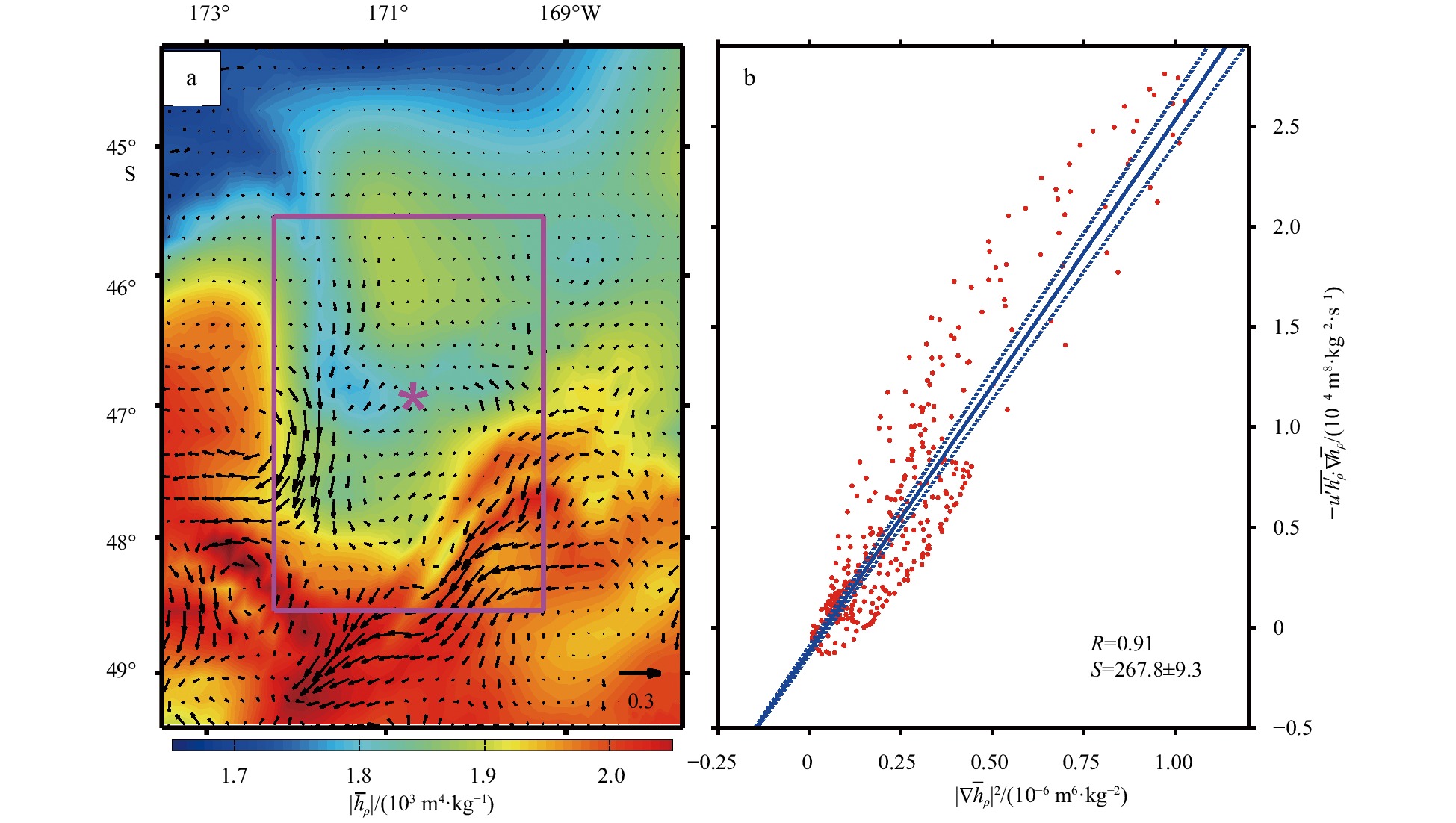
The local mesoscale fluctuation is not only associated with the local large-scale gradient, but also influenced by upstream and downstream advection, especially in the Southern Ocean (Chen et al., 2014), therefore, the linear regression analysis is used to obtain the eddy diffusivity. It should be noted that the horizontal resolution of the SOSE data is (1/6)° by (1/6)°, it can distinguish the coherent mesoscale eddies. However, the data resolution is insufficient to portray the diffusion process in coherent mesoscale eddies which is on a smaller scale. Therefore, the $ \kappa $ calculated in this study does not include the diffusion process in coherent mesoscale eddies. The diffusion process is introduced by parameterization during model operation. Take the 30th isoneutral layer (27.65–27.70 kg/m³, equivalent to 1 096.8 m to 1 521.5 m in Cartesian coordinate) for illustration, the eddy thickness flux ($\overline {{\boldsymbol{u}}'{{h'_\rho }}}$, black arrows) and magnitude of the large-scale thickness gradient ($ \left| {\nabla {{\bar h}_\rho }} \right| $, color) is shown in Fig. 1a. The magenta asterisk represents the calculation target point, and the rectangular area (3° by 3°) is the calculation region in the linear regression analysis. Figure 1b displays the calculation of the eddy diffusivity at the magenta-asterisk location shown in Fig. 1a. The eddy diffusivity is defined as the linear regression coefficient (the blue line in Fig. 1b), and it is (267.8±9.3) m²/s for the magenta asterisk in Fig. 1a. Applying this method in each isoneutral layer, the three-dimensional eddy diffusivity ($\kappa = \kappa (x{\rm{,}}y{\rm{,}}{z_\rho })$) can be obtained in which x, y, $ {z_\rho } $ denote longitude, latitude and isoneutral layer, respectively.

Figure  1.  Calculation of eddy diffusivity at the 30th isoneutral layer (27.65–27.70 kg/m³) by the linear regression analysis. a. Distribution of mesoscale thickness flux (black arrows, unit: m⁵/(kg·s)) and magnitude of large-scale isoneutral thickness gradient (color, unit: 10³ m⁴/kg) at the 30th isoneutral layer. The magenta asterisk and rectangular area (3° by 3°) indicate the calculation target point and calculation region, respectively. b. Linear regression of eddy diffusivity at the center of the magenta box in Fig. 1a. The abscissa is the square of the large-scale thickness gradient (unit: 10⁻⁶ m⁶/kg²), and the ordinate represents the inverse of the product of mesoscale thickness flux and large scale thickness gradient (unit: 10⁻⁴ m⁸/(kg²·s)). The blue dashed lines are the boundaries of the 95% confidence interval. The symbols “S” and “R” are the linear regression coefficient and Pearson correlation coefficient, respectively.

DownLoad: Full-Size Img PowerPoint

2.3 Coherent eddy detection and tracking method

The automated two-dimensional coherent mesoscale eddy detection and tracking algorithm (Nencioli et al., 2010) is adopted in this study. This algorithm is based on the velocity geometric characteristics of the coherent mesoscale eddy, and has been successfully applied to many researches (Couvelard et al., 2012; Aguiar et al., 2013; Dong et al., 2014; Ji et al., 2017; Liu et al., 2017; Sun et al., 2018, 2019; Yang et al., 2020). Simply, this algorithm contains three steps:

First step: locating the two-dimensional coherent mesoscale eddy center which satisfies the following four geometrical constraints.

(1) The meridional velocity ($ v' $) changes its sign across a coherent mesoscale eddy center, and its magnitude increases away from the center along the zonal direction.

(2) Similar to (1), the zonal velocity ($ u' $) has opposite signs across a coherent mesoscale eddy center, and its magnitude also increases away from the center but along the meridional direction.

(3) The horizontal velocity ($ \sqrt {{{u'}^2} + {{v'}^2}} $) should be locally minimum in a coherent mesoscale eddy center.

(4) Construct a local two-dimensional Cartesian coordinate system with the origin as a possible coherent mesoscale eddy center. The abscissa and ordinate denote zonal and meridional directions, respectively. In two adjacent or the same quadrants, the direction of the velocity vector $ (u'{{,}}v') $ must change with the same trend, i.e., the velocity constitutes a clockwise or anticlockwise flow pattern. In order to get a better performance, velocity data are linearly interpolated onto a (1/12)° by (1/12)° grid before applying this eddy detection method.

Second step: defining the eddy boundary for each eddy center. In this study, the outermost contour of the local stream function, which encloses a coherent mesoscale eddy center, is defined as the eddy boundary.

Third step: two-dimensional coherent eddy tracking. Considering the temporal resolution of the SOSE data (5 d) and average velocity of the background field in the Southern Ocean (about 0.15 m/s), a circular search area with a 1.2° radius is chosen to track the coherent mesoscale eddy. If a two-dimensional coherent eddy is successfully detected at time step $ t $, the coherent mesoscale eddy with same polarity (cyclonic or anticyclonic) will be searched for at the next time step $ t + 1 $ within the search area. If more than one eddies fit the criteria, the nearest eddy is identified as the well-defined eddy. If no coherent mesoscale eddy is found within the search area, a second search is conducted at time step $ t + 2 $ within a larger circular search area (1.8° radius). This coherent mesoscale eddy is considered as “disappeared” if there is still no eddy detected at time step $ t + 2 $. The eddy lifespan is defined as the period from the search beginning time step to the last successful detection time step, and it must be multiple of 5 due to the time interval of the SOSE data.

Applying this eddy automated detection method to each vertical layer, discrete two-dimensional coherent mesoscale eddies datebase is obtained. Figure 2 shows a sample distribution of two-dimensional coherent mesoscale eddies in an arbitrary area of the Southern Ocean at sea surface on February 25, 2005. The blue (red) curves indicates the boundaries of coherent mesoscale cyclonic (anticyclonic) eddies. The black asterisks indicate the eddy centers. There are abundant coherent mesoscale eddies in the Southern Ocean, and this method can successfully identify them.

Figure  2.  A snapshot of coherent mesoscale eddies on February 25, 2005 in an arbitrary area of the Southern Ocean at sea surface. Black asterisks indicate the coherent mesoscale eddy centers. Blue and red curves represent the boundaries of coherent mesoscale cyclonic eddies and anticyclonic eddies, respectively. Black vectors correspond to velocity anomalies. The two eddies with bold dotted boundaries are analyzed in Subsection 5.1 and shown in Fig. 6.

DownLoad: Full-Size Img PowerPoint

The three-dimensional eddy detection method (Dong et al., 2012) is also used. This method is based on three conditions: (1) the same eddy should have the same occurrence time at each level; (2) the same eddy also should have the same polarity at each level; (3) the drift distance of the eddy center is no farther than a quarter of its radius between two neighboring vertical levels. The eddy center is iterated downward until the new eddy center cannot be found at the next level. Finally, a three-dimensional coherent mesoscale eddy dataset is produced, which contains coherent mesoscale eddy polarity, generated time, vertical penetration depth, radius (defined as the radius of a circle that has the same area with the recognized eddy), center and horizontal boundary at each level.

2.4 Uncertainties and limitations due to SOSE data resolution

Three screening conditions are introduced in this study to reduce uncertainties in different detection and tracking methods of the coherent mesoscale eddies: (1) considering that the characteristic time scale of the coherent mesoscale eddies is in several weeks, only the eddies surviving equal to or longer than 30 days are selected; (2) since the spatial scale of the coherent mesoscale eddies is O (100 km)–O (50 km) from 30°S to 65°S (Chelton et al., 2011) and the model resolution is (1/6)° by (1/6)°, only the eddies with an average radius larger than 30 km are singled out; (3) for a better representation of the coherent mesoscale eddies, only the eddies with a vertical penetration depth more than 100 m are selected.

3. Data validation

Derived from the SOSE data, the sea surface height anomaly (SSHA) is negative in high latitude and positive in low latitude of the Southern Ocean (Fig. 3a), and it is consistent with the AVISO SSHA (Fig. 3b). The multi-year and spatial average SSHA from SOSE (AVISO) is (−0.23±0.66) m ((0.0 ± 0.65) m). The variance of the SOSE data is 0.04 m² compared with the AVISO data. In addition, the sea surface eddy kinetic energy (EKE) also shows good agreement between the two datasets (Figs 3c and d). The sea surface EKE is energetic to the north of the Subpolar Antarctic Front (SAF), and weak on the southern side of the Antarctic Front (AF, Fig. 3d). In this study, the SAF is defined as the 4°C isotherm at 200 m depth (Orsi et al., 1993), and the AF is defined as the location with the minimum salinity at 200 m depth (Gordon et al., 1978). The average sea surface EKE is (136.5±256) cm²/s² from the SOSE data, which is slightly lower than the AVISO result ((169.7±265) cm²/s²). Compared with the AVISO data, the variance of the sea surface EKE from the SOSE data is 6.3 cm⁴/s⁴. In addition, the probability density distribution of the SSHA and EKE is also calculated, and similar results are obtained between the two datasets (figure not shown), further confirming the reliability of SOSE data.

Figure  3.  Distribution of multi-year (2005–2010) average sea surface height anomaly (SSHA) (a, b) and sea surface eddy kinetic energy (EKE) (c, d), calculated from SOSE data (a, c) and AVISO data (b, d). The blue and red curves in a and c denote the multi-year average position of the Subpolar Antarctic Front and Antarctic Front, respectively.

DownLoad: Full-Size Img PowerPoint

4. Distribution of eddy diffusivity

The spatial distribution of the eddy diffusivity in the Southern Ocean is shown in Fig. 4. Figures 4a and b are displayed in the isoneutral coordinate system, corresponding to the 27.15–27.20 kg/m³ and 27.95–28.00 kg/m³ isoneutral layers. Figures 4c and d are displayed in the Cartesian coordinate system, corresponding to 60–72 m and 826–1 092 m layers. In general, the magnitude of the eddy diffusivity is on the order of O (10³ m²/s), which is close to the typical value applied in non-eddy-resolving ocean models. However, as noted in Fig. 4 and some previous literature (Gent, 2011; Lu et al., 2016; Bachman et al., 2020; Stanley et al., 2020), the eddy diffusivity has noticeable spatial variation. Positive eddy diffusivity implies the local production of EKE obtaining energy from large-scale mean flow. On the contrary, negative eddy diffusivity corresponds to the mesoscale eddy releasing energy to large-scale mean flow (Eden et al., 2007). The distribution of negative eddy diffusivity is irregular (Fig. 4a), this may be related to the fact that the negative eddy diffusivity is influenced by several processes, such as the rotational eddy flux (Marshall and Shutts, 1981; Bryan et al., 1999; Medvedev and Greatbatch, 2004; Eden et al., 2007), advection of thickness variance and enstrophy (Treguier et al., 1997; Bachman and Fox-Kemper, 2013), and stationary mesoscale eddy flux (Lu et al., 2016). Besides, Marshall et al. (2006) believed that the estimated eddy diffusivity more accurately corresponds to the dianeutral thickness diffusivity in the upper layer. Figure 5 shows that the negative eddy diffusivity mainly appears in the upper layer of the ocean indeed, in agreement with Marshall et al. (2006). That is, the negative value represents the occurrence of the dianeutral process, indicating that the original calculation Eq. (3) cannot be accurately established. This is an interesting and important issue but is beyond our present scope.

Figure  4.  Spatial distribution of the eddy diffusivity in the Southern Ocean. (a) and (b) correspond to 27.15–27.20 kg/m³ and 27.95–28.00 kg/m³ layers in the isoneutral coordinate system, (c) and (d) correspond to 60–72 m and 826–1 092 m layers in the Cartesian coordinate system. Colors represent the eddy diffusivity (unit: 10³ m²/s). The blue and red curves are the multi-year average position of the Subpolar Antarctic Front (SAF) and Antarctic Front (AF), respectively.

DownLoad: Full-Size Img PowerPoint

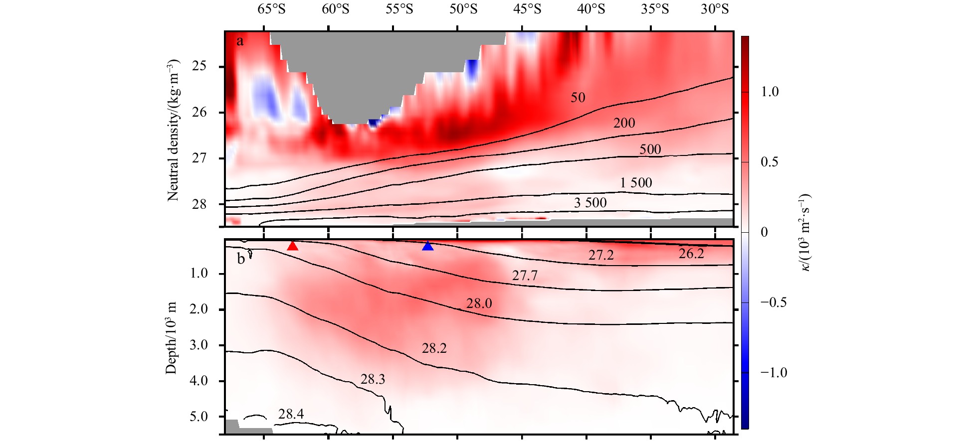
Figure  5.  Zonal mean of the multi-year (2005–2010) average eddy diffusivity in isoneutral coordinate system (a) (unit: 10³ m²/s) and Cartesian coordinate system (b). The mean isobaths (50 m, 200 m, 500 m, 1 500 m and 3 500 m) and mean isoneutral contours (26.2 kg/m³, 27.2 kg/m³, 27.7 kg/m³, 28.0 kg/m³, 28.2 kg/m³, 28.3 kg/m³ and 28.4 kg/m³) are labeled in a and b, respectively. The blue and red triangles in b are the multi-year average position of the Subpolar Antarctic Front and Antarctic Front, respectively.

DownLoad: Full-Size Img PowerPoint

Although the results in this study are similar to those in previous literature, there are some differences in the calculation method of eddy diffusivity. (1) This study uses the isoneutral coordinate system, which is closer to the real physical process in the ocean, compared with the Cartesian coordinate system (Eden et al., 2007) and potential density coordinate system (Bryan et al., 1999; Lu et al., 2016); (2) normalized thickness of the isoneutral layer is adopted as a passive tracer to calculate the eddy diffusivity in this study, instead of buoyancy (Treguier et al., 1997; Eden et al., 2007), and potential vorticity (Marshall et al., 2012; Bachman et al., 2017); (3) the linear regression in a 3° by 3° box is performed to calculate the eddy diffusivity. This method can avoid the division issue that the denominator is close to zero; (4) the temporal-spatial filtering scheme is adopted in this study, this can avoid the influence of Leonard and Clark terms more easily, compared with the spatial filtering method (Bachman and Fox-Kemper, 2013); (5) compared with the derived tracer transport (Marshall et al., 2006), which only gave the surface eddy diffusivity in the Southern Ocean, this study further demonstrates the vertical distribution of the eddy diffusivity.

Figure 5 is the zonal mean of the eddy diffusivity in the isoneutral coordinate system (Fig. 5a) and Cartesian coordinate system (Fig. 5b). In the meridional direction, the eddy diffusivity is obviously larger between the northern flank of the SAF (about 52.3°S) and about 40°S (Fig. 5a). In the vertical direction, the eddy diffusivity is mainly concentrated within the upper 50 m, and then it rapidly decays with depth. These distribution characteristics of the eddy diffusivity are consistent with Eden et al. (2007).

By converting the results from the isoneutral coordinate to the Cartesian coordinate system, the eddy diffusivity is obviously higher under the SAF and AF region (Fig. 5b). The enhanced area reaches about 3 000-m depth (near the 28.3 kg/m³ isoneutral level). Abernathey et al. (2010) suggested that this phenomenon is attributed to a “critical layer” in which the eddy phase speed equals the mean flow speed. Besides, the deeper vertical penetration depth and stronger intensity of the coherent mesoscale eddies are also found to be important in this study. For a more detailed description, please refer to Subsection 5.5. To sum up, the eddy diffusivity is on the order of O (10³ m²/s) and shows an evident spatial variation in the Southern Ocean.

5. Basic characteristics of coherent mesoscale eddies

5.1 Three-dimensional structure of coherent mesoscale eddy cases

Two cases of the eddies (with bold dotted boundaries in Fig. 2) are selected, and their three-dimensional structures (Figs 6a and c) and vertical distributions of the normalized eddy intensity (Figs 6b and d) are shown in Fig. 6. The radius of the coherent mesoscale cyclonic (anticyclonic) eddy is 96.5 km (72.6 km) at sea surface, and almost keeps unchanged to its bottom (about 1 173.5 m, Figs 6a and c). The vertical penetration depth of the coherent mesoscale eddy is 1 173.5 m, as the automated eddy detection program could not detect the presence of the eddy in the next layer (1 348.5 m) below 1 173.5 m. Below 900 m, the temperature anomalies become very small and is almost negligible for both coherent mesoscale cyclonic eddy and anticyclonic eddy (xoz and yoz coordinate plane in Figs 6a and c). In a word, coherent mesoscale eddy-induced temperature anomalies decrease with depth, while the radius has less change from surface to 1 173.5 m.

Figure  6.  Three-dimensional structures of two coherent mesoscale eddy cases (a, c) and their vertical eddy intensity distributions (b, d). The meridional (zonal) temperature anomalies across the eddy center are shown in $ xoz $ ($ yoz $) coordinate plane. (a) and (b) are for the cyclonic eddy, (c) and (d) are for the anticyclonic eddy. Colors represent potential temperature anomaly (unit: °C), which is the deviation from the large-scale average using a temporal-spatial filtering method. The blue and red curves indicate the boundaries of the coherent mesoscale cyclonic and anticyclonic eddy on the two-dimensional layers, which is defined as the outermost enclosed local stream function. White vectors indicate velocity anomaly (unit: m/s), and grey outlines are the three-dimensional boundary of the eddy. Black asterisks indicate the eddy centers. Black dashed lines in b and d indicate one standard deviation.

DownLoad: Full-Size Img PowerPoint

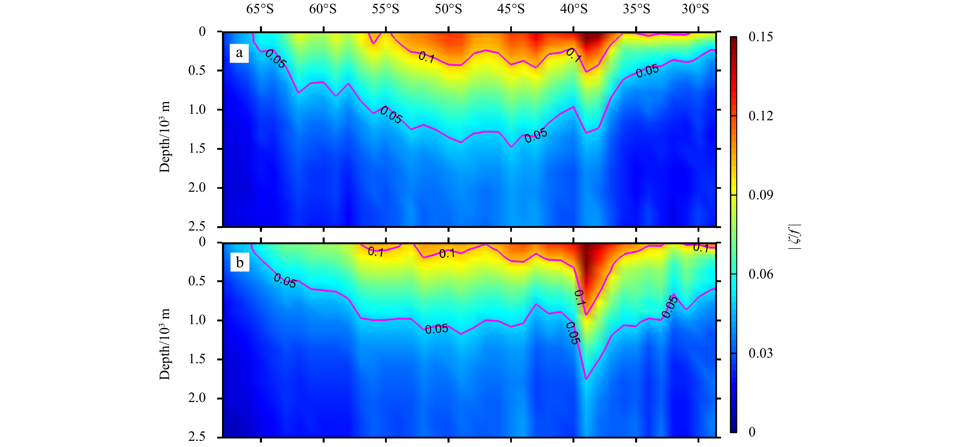
The intensity of coherent mesoscale eddies can be expressed by several physical parameters, such as EKE, relative vorticity and deformation rate. These parameters reflect the characteristics of a coherent mesoscale eddy from different aspects. Considering the wide latitude span of the Southern Ocean, $ {\gamma _I} = \left| {\dfrac{\zeta }{f}} \right| $ is chosen as its intensity, where $ \zeta = \dfrac{{\partial v'}}{{\partial x}} - \dfrac{{\partial u'}}{{\partial y}} $ is the relative vorticity averaged within the eddy and $\, f $ is the local planetary vorticity, also represents Coriolis parameter. For both coherent mesoscale cyclonic eddy and anticyclonic eddy, $ {\gamma _I} $ decreases rapidly with depth, reaching less than half of the surface value at 900 m. The maximum $ {\gamma _I} $ is 0.17 for the coherent mesoscale cyclonic eddy and 0.13 for the anticyclonic eddy, both of them are less than 20% of the local planetary vorticity.

5.2 Number of coherent mesoscale eddies

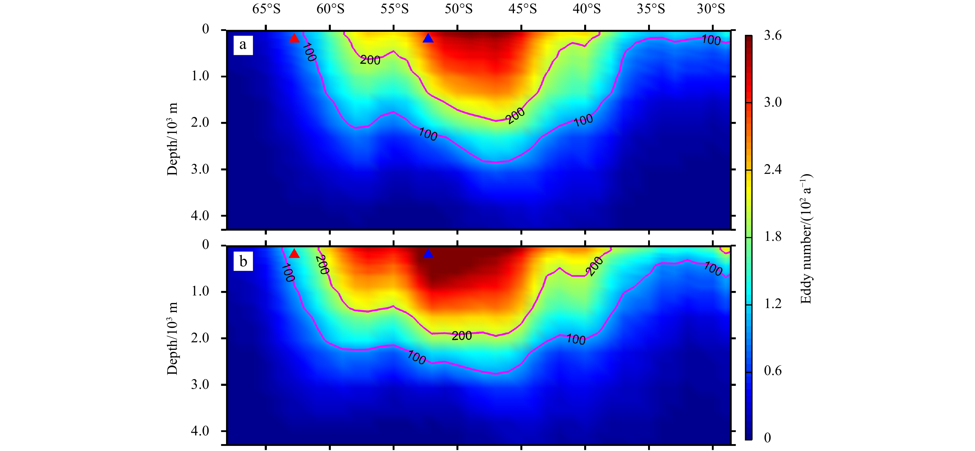
There are two methods to calculate the number of coherent mesoscale eddies. One is the eddy lifespan counting (ELC) method: a whole lifespan of successive coherent mesoscale eddies is considered as one eddy (Chelton et al., 2011; Chen et al., 2012; Aguiar et al., 2013). The other one is the eddy snapshot counting (ESC) method: the eddy number depends on how many coherent mesoscale eddies are identified from each snapshot (Chen et al., 2011; Dong et al., 2012; Frenger et al., 2013; He et al., 2018; Sun et al., 2018; Yang et al., 2020). The number of coherent mesoscale eddies recognized by the ESC method reflects the frequency of eddies occurring at a certain spatial location during the statistical time period. A larger number (i.e., more eddies identified by the ESC method) indicates a higher frequency or probability of eddies appearing at this location. In general, the coherent mesoscale eddies tend to travel long distances throughout their lifespan (Chelton et al., 2011). The ELC method can only reflect the average position of eddies, but cannot accurately find the position with higher/lower probability of eddies. In addition, the radius, intensity and vertical penetration depth of the eddy are constantly changing during its lifetime (Sun et al., 2018). The ELC method may regard several eddy snapshots in the whole lifespan as one eddy, which cannot accurately reflect the spatial and temporal changes of the above-mentioned characteristics of the eddy. Therefore, the ESC method is used in this study, except when calculating the lifespan of the coherent mesoscale eddy. During 2005–2010, eddies are concentrated between the northern side of the SAF to 45°S for both coherent mesoscale cyclonic eddies (Fig. 7a) and anticyclonic eddies (Fig. 7b). The maximum eddy number appears at 47°S for coherent mesoscale cyclonic eddy (361.2±4.7) a⁻¹ and 51°S for coherent mesoscale anticyclonic eddy (414.3±5.6) a⁻¹. In upper 3 000 m, the eddy number between the northern side of the SAF to 45°S is significantly larger than in other regions. This implies that more coherent mesoscale eddies reside and penetrate more deeply in this area. A more detailed description of the eddy penetration depth is given in Subsection 5.5.

Figure  7.  Number of multi-year (2005–2010) average coherent mesoscale cyclonic eddy (a) and anticyclonic eddy (b) based on the eddy snapshot counting method. Colors represent the number of coherent mesoscale eddies (unit: 10² a⁻¹). The blue and red triangles are the position of the multi-year average Subpolar Antarctic Front and Antarctic Front, respectively. The magenta curves indicate the contours with eddy numbers of 100 a⁻¹ and 200 a⁻¹.

DownLoad: Full-Size Img PowerPoint

5.3 Radius of coherent mesoscale eddies

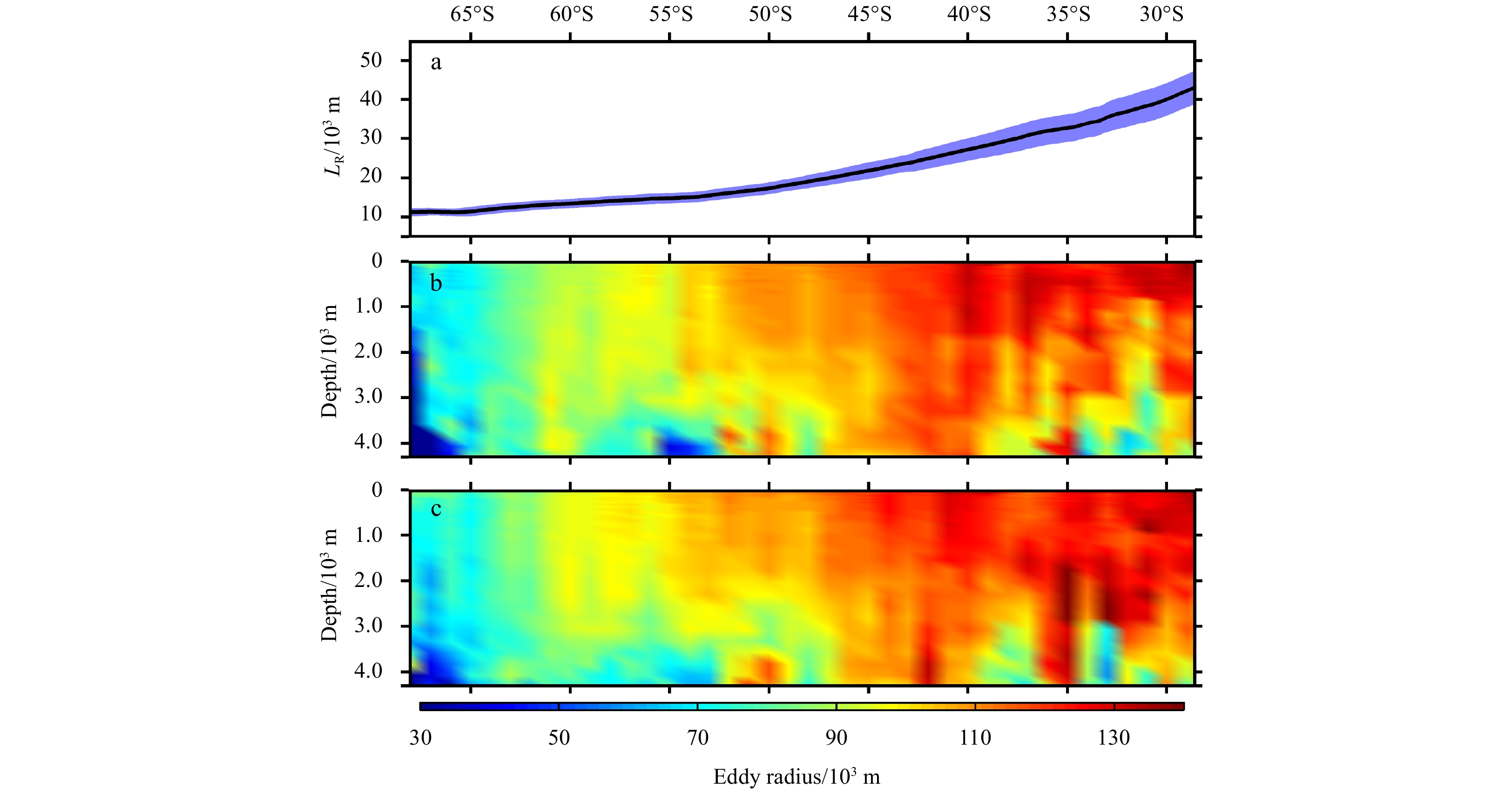
In the open ocean, the radius of coherent mesoscale eddies is mainly constrained by the first baroclinic Rossby deformation radius ($ {L_{\rm{R}}} $; Stammer, 1997; Chelton et al., 2011; Klocker and Marshall, 2014). Definitely, the radius near the ocean bottom is also limited by topography. The first baroclinic Rossby deformation radius is calculated based on the the formula of ${L_{\rm{R}}} = \dfrac{{\dfrac{1}{\pi }\int_{ - H}^0 {N(z){\rm{d}}z} }}{{\left| f \right|}}$ (Chelton et al., 1998), where $ H $ is the water depth, $ N(z) $ is the buoyance frequency, and $\, f $ is the local planetary vorticity. It gradually increases from (11.5±1.2) km at 65°S to (39.7±4.2) km at 30°S (Fig. 8a). For both the cyclonic eddy and anticyclonic eddy, the radius shows simimar meridional variation (Figs 8b and c). At sea surface layer, the radius of coherent mesoscale cyclonic (anticyclonic) eddies increases from (43.9±5.3) km ((44.7±4.9) km) at 65°S to (121.2±10.4) km ((117.8±9.6) km) at 30°S (Figs 8b and c). The value is nearly three times larger than the first baroclinic Rossby deformation radius. There are two possible reasons for this phenomenon. First, three additional restrictions are added to the detected eddies in this study, so that some eddies with smaller radii are removed (Subsection 2.4). The other reason is related to the chosen of eddy boundary. The eddy bounadary is defined as the outermost closed stream function in this study (Subsection 2.3), so that the radius is almost two times larger than that derived from the maximum flow position method. The radius of coherent mesoscale eddies with respect to latitude becomes complex below about 2 000 m. This change may be attributed to the topography at the ocean bottom.

Figure  8.  Distribution of the multi-year (2005–2010) average first baroclinic Rossby deformation radius (a) and eddy radius of coherent mesoscale cyclonic eddies (b) and anticyclonic eddies (c). The blue shaded area in a represents one standard deviation. Colors in b and c represent the radius of the coherent mesoscale eddy (unit: 10³ m).

DownLoad: Full-Size Img PowerPoint

5.4 Intensity of coherent mesoscale eddies

As discussed in Subsection 5.1 (Figs 6b and d), the larger eddy intensity is mostly concentrated in the upper ocean (Fig. 9). For cyclonic eddies (Fig. 9a), the normalized intensity greater than 0.1 is concentrated in the upper 500 m between 57°S to 35°S. The 0.05-isoline of the normalized intensity exhibits a bowl-shaped distribution, which is the deepest (about 1 500 m) around 50°S to 45°S, and gradually shoals to the north and south sides. However, for anticyclonic eddies (Fig. 9b), there seems an abrupt deepening of 0.1-isoline and 0.05-isoline around 38°S, indicating the most enegetic anticyclones here. Actually, the similar abrupt deepening also occurs for cyclonic eddies, but with a weaker magnitude. Such a boom of the eddy intensity around 38°S deserves further investigation in the future.

Figure  9.  Distribution of multi-year (2005–2010) average intensity for coherent mesoscale cyclonic eddies (a) and anticyclonic eddies (b). Colors represent the normalized intensity. The magenta curves indicate the isolines with the eddy intensity of 0.05 and 0.1, respectively.

DownLoad: Full-Size Img PowerPoint

5.5 Penetration depth and lifespan of coherent mesoscale eddies

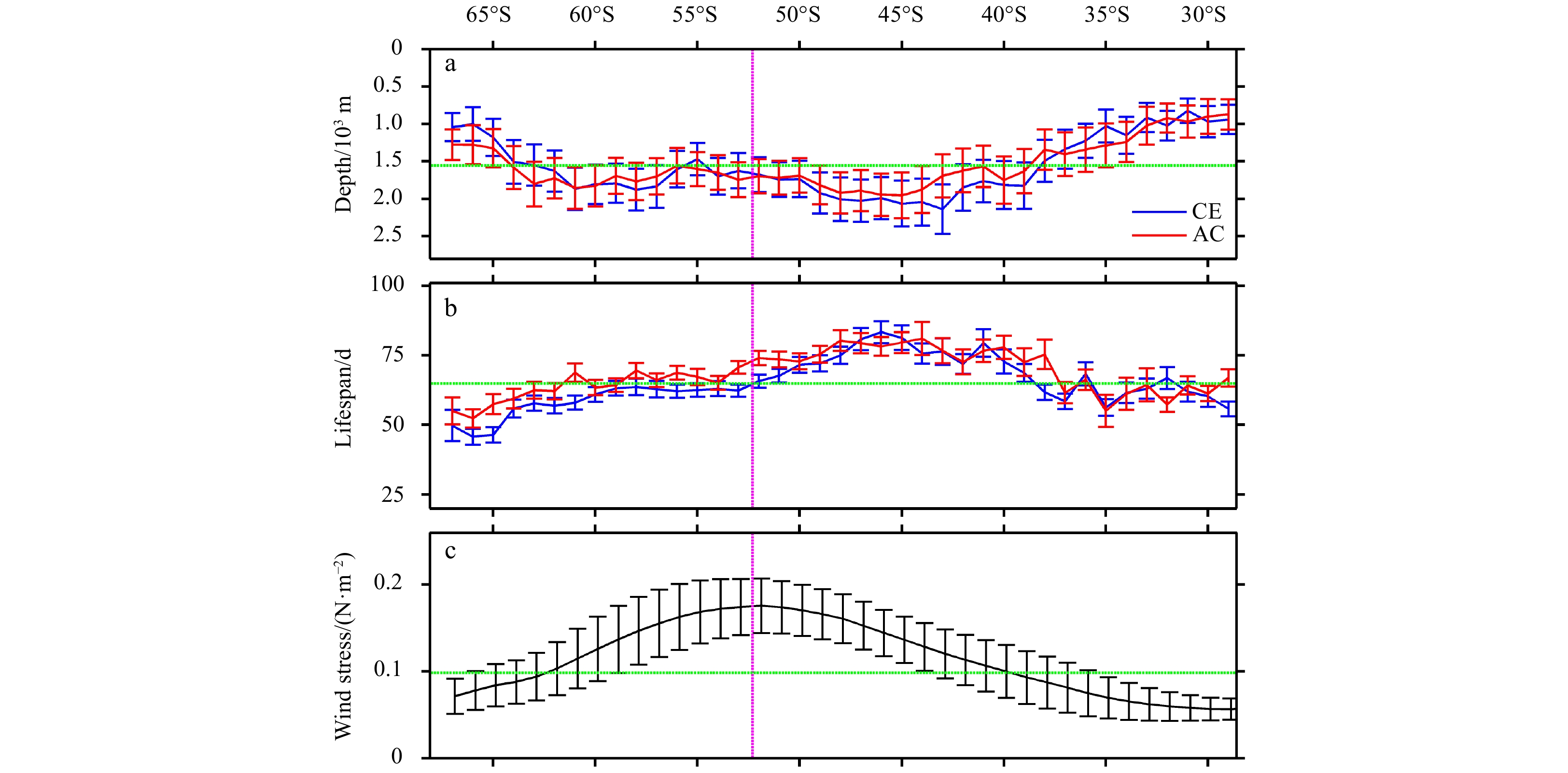
It can be inferred from Fig. 7 that the vertical penetration depth of coherent mesoscale eddies is deeper in the SAF and its northern region than in other regions, and it is confirmed in Fig. 10a. The multi-year average maximum penetration depth of the coherent mesoscale cyclonic eddy is (2 139.5±329.1) m at 43°S, and it is (1 953.6±304.1) m at 45°S for anticyclonic eddy.

Figure  10.  Distribution of multi-year (2005–2010) average of coherent mesoscale eddy penetration depth (a), lifespan (b) and wind stress (c). The blue and red curves are for coherent mesoscale cyclonic and anticyclonic eddies, respectively. The error bar is also shown in the figure. The green dotted lines are the meridional average eddy penetration depth, eddy lifespan for all coherent mesoscale eddies and wind stress. The magenta dotted line is the multi-year average latitude of the Subpolar Antarctic Front.

DownLoad: Full-Size Img PowerPoint

The lifespan of coherent mesoscale eddies also changes with latitude (Fig. 10b). It is worth noting that only the eddies surviving more than 30 days are retained in this study (Subsection 2.4). Consistent with the penitration depth, the lifespan of the coherent mesoscale eddy (both cyclonic and anticyclonic) between the SAF and 38°S is longer than that in other areas as well. The multi-year average longest lifespan of the coherent mesoscale cyclonic eddy is (83.3±3.9) d at 46°S, and it is (81.0±5.9) d at 44°S for anticyclonic eddy.

The most immediate cause of this phenomenon (i.e., deeper penetration depth and longer survival time between the northern side of the SAF to 38°S) may be attributed to the larger local wind stress in this region (Fig. 10c). The Pearson correlation coefficient between normalized wind stress and normalized cyclonic (anticyclonic) eddy penetration depth is 0.69 (0.74). This implies that the coherent mesoscale eddies is more vigorous in this region, which can be also inferred from the distribution of sea surface EKE in Fig. 3d.

6. Relationship between normalized eddy diffusivity and coherent mesoscale eddy activity

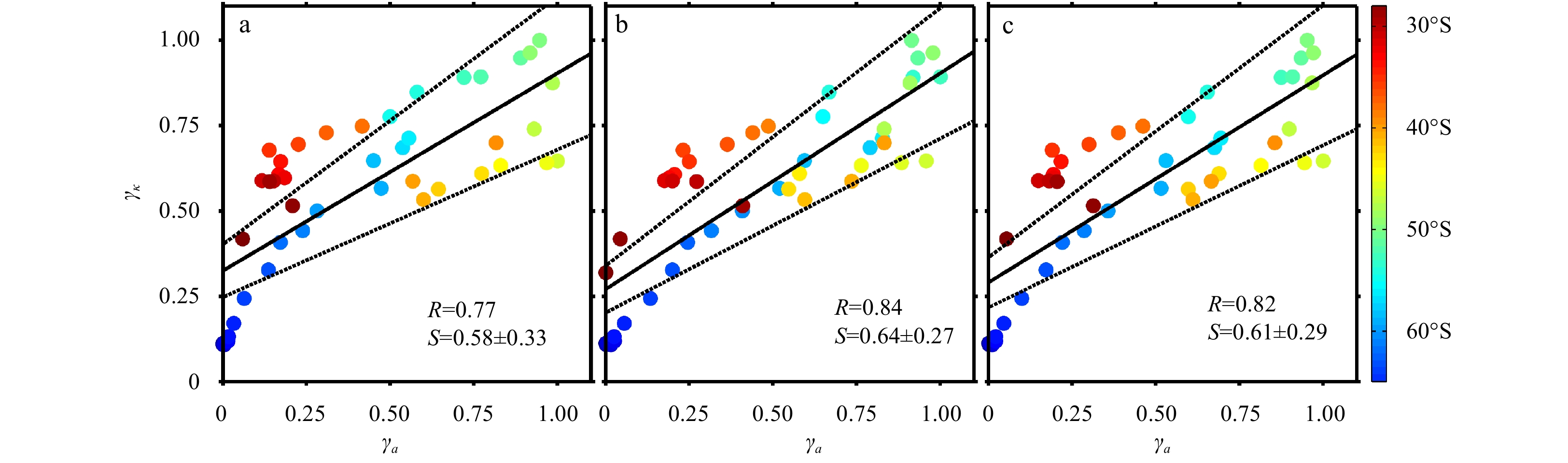
The scatterplots of normalized eddy activity ($ {\gamma _a} $) and normalized eddy diffusivity ($ {\gamma _k} $) are shown in Fig. 11. The normalized eddy activity is defined as ${\gamma _a} = \dfrac{{\dfrac{{{\gamma _I}}}{{\max ({\gamma _I})}} \times \dfrac{{{E_n}}}{{\max ({E_n})}}}}{{\max \left[\dfrac{{{\gamma _I}}}{{\max ({\gamma _I})}} \times \dfrac{{{E_n}}}{{\max ({E_n})}}\right]}}$, where $ {\gamma _I} $ is the eddy intensity in each latitude band ($ {\gamma _I} = \left| {\dfrac{\zeta }{f}} \right| $, Subsection 5.1), and $ \max ({\gamma _I}) $ is the maximum of eddy intensity in the total latitude bands. Similarly, $ {E_n} $ is the coherent mesoscale eddy number in each latitude band and $ \max ({E_n}) $ is the maximum of coherent mesoscale eddy number in all of the latitude bands. The normalized eddy diffusivity is defined as: ${\gamma _k} = $$ \dfrac{{\dfrac{1}{V}\iiint\limits_V {\kappa {\rm{d}}V}}}{{\max \left(\dfrac{1}{V}\iiint\limits_V {\kappa {\rm{d}}V}\right)}}$, where the numerator is volume-averaged diffusivity in each latitude band, and the denominator is the maximum of volume-averaged diffusivity in all of the latitude bands. The lower limit of the vertical integration is 2 000 m, considering that the average penetration depth is generally shallower than that depth (Fig. 10a).

Figure  11.  Scatter plots of normalized eddy activity against normalized eddy diffusivity for coherent mesoscale cyclonic eddies (a), anticyclonic eddies (b), and all the eddies regardless of polarity (c) . The symbols “S” and “R” are the slope of the regressed line (black line) and Pearson correlation coefficient, respectively. The colors represent latitudes, and the dashed black lines are the boundaries of the 95% confidence interval.

DownLoad: Full-Size Img PowerPoint

Overall, the normalized eddy activities of coherent mesoscale cyclonic eddies (Fig. 11a), anticyclonic eddies (Fig. 11b) and all the eddies regardless of polarity (Fig. 11c) have a significant positive correlation with the normalized volume-averaged eddy diffusivity. The slope of the regressed line is 0.58$ \pm $0.33, 0.64$ \pm $0.27, 0.61$ \pm $0.29 and the Pearson correlation coefficient is 0.77, 0.84, 0.82, for coherent mesoscale cyclonic eddies, anticyclonic eddies and all the eddies, respectively. Considering that many ocean processes (such as mesoscale fronts, mesoscale filaments and meanders) could affect eddy diffusivity, this result provides a potential reference direction to improve the parameterization schemes of mesoscale eddy in the future. If the strength and structure characteristic of coherent mesoscale eddy could be taken into consideration, the accuracy of mesoscale eddy parameterization is believed to be improved.

7. Summary and conclusions

This study focuses on three issues: (1) the distribution of eddy diffusivity; (2) the basic characteristics of coherent mesoscale eddy; and (3) the relationship between coherent mesoscale eddy and eddy diffusivity in the Southern Ocean. Based on the SOSE data and linear regression analysis, the three-dimensional structure of eddy diffusivity is revealed. All the calculations of eddy diffusivity are carried out in an isoneutral coordinate system. This study finds that the eddy diffusivity is on the order of O (10³ m²/s) and has an evident spatial variation in the Southern Ocean.

Through two coherent mesoscale eddy cases, it is found that the radius of the coherent mesoscale eddy can be maintained unchanged to deeper than 1 000 m in vertical direction, while the eddy-induced temperature changes are concentrated in upper 900 m. The coherent mesoscale eddies are concentrated from the northern side of the SAF to 45°S. The average penetration depth is deeper and the lifespan is longer in this area than in other areas. In the upper ocean, the radius of the coherent mesoscale eddy (both cyclonic and anticyclonic) is associated with the first baroclinic Rossby deformation radius. Attributed to the effects of the bottom topography in the Southern Ocean, the variation of the eddy radius with latitude is more complex below about 2 000 m.

The intensity of coherent mesoscale eddy is mainly concentrated in the upper ocean, and its normalized value is less than 0.05 deeper than 1 500 m. The average vertical penetration depth of the eddy is also about 1 500 m. The normalized coherent mesoscale eddy activity and the normalized eddy diffusivity have a good linear correlation. Moreover, the coherent mesoscale eddy may plays an important role in eddy diffusivity.

Investigating the spatial distribution of eddy diffusivity and the basic characteristics of coherent mesoscale eddies enriches our understanding of mesoscale processes. Explanation of the relationship between coherent mesoscale eddies and eddy diffusivity is helpful to figure out the contribution of coherent mesoscale eddies to eddy diffusivity. Besides, it also provides a reference for the improvement of mesoscale eddy parameterization schemes.

Acknowledgements

The Southern Ocean State Estimate (SOSE) data are downloaded from http://sose.ucsd.edu/sose_stateestimation_data_08.html, and computational resources for SOSE are supported by NSF XSEDE resource grant (OCE130007). The altimeter products are produced by the Ssalto/Duacs and distributed by AVISO, with support from the Centre National d’Etudes Spatiales (http://www.aviso.oceanobs.com/duacs/). We thank Hailong Liu (Institute of Atmospheric Physicals, Chinese Academy of Sciences), Jianhua Lu (Sun Yat-Sen University) and Fuchang Wang (Shanghai Jiao Tong University) for the constructive discussion. We thank Matthew Mazloff (Scripps Institution of Oceanography) for the kindly help in data download. We also thank two anonymous reviewers for their constructive comments and helpful suggestions.