The influence of Stokes drift on oil spills: Sanchi oil spill case

1. Introduction

There are two types of marine oil spills, the first is oil spilled from production platforms such as the Deepwater Horizon oil spill in the Gulf of Mexico (Dietrich et al., 2012), and Penglai 19-3 oil spill in the Bohai Sea (Yang et al., 2017). The second is oil spilled from ships such as after the Sanchi collision accident in the East China Sea (Li et al., 2019), or the Hebei Spirit oil tanker accident (Kim et al., 2014). According to ITOPF (The International Tanker Owners Pollution Federation), over the last 50 years (1970–2019) more than 450 recorded ship oil spills have been recorded, with the majority resulting from tanker collisions (31%) and groundings (26%). Due to the improvement of technology, as well as ship and marine related policies, the number of large spills has continued to decrease over the last 50 years. The yearly average recorded this decade is 1.8 spills, less than a tenth of the average recorded in the 1970s.

Oil spilled in marine and coastal waters and marine can significantly contaminate aquatic environments, damaging ecosystems and detrimentally influencing associated economies. Although the number of large oil spill accidents (>700 t) is continuing to decrease, it remains a significant source marine pollution. The prediction of an oil spill trajectory, a contamination area, and a swept area is crucial for an accurate environmental impact assessment. Numerical models are currently the main technical method utilized in predicting oil spills, and are used extensively in oil spill research and operational forecasting. After an oil spill has occurred, it is essential to rapidly and accurately predict the movement of oil slicks, to allow for the protective and mitigative damage (Kim et al., 2014).

Once oil has been spilled into the marine environment, its movement is governed by a complex of physical and chemical processes which include drifting and weathering (Reed et al., 1999). Oil is advected by the surface currents associated with tides, riverine discharge, oceanographic currents, meteorological forcing, breaking waves, and by direct wind forcing at the sea surface (Dietrich et al., 2012). Spreading, evaporation, emulsification, and dispersion are important oil weathering processes that are influenced by currents, winds, wave action, water temperature, and the type of spilled oil.

Winds also play a significant role by defining surface velocities. Observational data suggests that the wind drift velocity of oil particles is 1%–6% that of the wind speed (Lehr and Simecek-Beatty, 2000). The influence of Stokes drift is significant as it often serves as an intensification of the wind effect (Deng et al., 2013), of the order of 1% of the wind speed (Ardhuin et al., 2018, 2009). Oil spill emergency forecasting is concerned with the drift of the oil spill on the ocean surface and as such the influence Stokes drift should not be ignored.

Waves are an important form of motion, generated by wind acting directly on the sea surface. Due to the existence of surface gravity waves, the nonlinear effect of Stokes drift leads to the non-closed trajectory of sea surface water points. Stokes drift is a phenomenon that occurs in the upper ocean layer in response to wind, waves, and currents, and it affects the transportation of plastics, oil, and pollution (Myrhaug et al., 2018; Ren et al., 2019). Stokes drift is the wave-averaged Lagrangian velocity that is derived from the water particle motion in the wave propagation direction. Its maximum velocity is at the surface, and decreases rapidly with the depth (Myrhaug, 2017).

There are two ways to calculate the Stokes drift at the surface, the first is determined from a one-dimensional frequency spectrum, and the second can be obtained from wave models based upon a two-dimensional spectrum. To extensively explain Stokes drift, a fully coupled ocean-wave model would be required. However, no operational coupled model and corresponding reanalysis was available for some time. In this study, the contribution of Stokes drift to an oil spill was analyzed. Three experiments were designed, the first only considered the influence of currents and wind, the second considered the influence of current, wind, and Stokes drift from an empirical formula, the third considered the same effect factors as the second but the Stokes drift was derived from an ocean-wave model.

2. Sanchi oil spill

On the 6th January 2018, the Iranian oil tanker Sanchi collided with the Hong Kong-flagged cargo ship in the East China Sea at 30°42′N, 124°56′E (Li et al., 2019; Qiao et al., 2019; Sun et al., 2018). The Sanchi tanker that was carrying a full cargo of 136 000 metric tons of natural gas condensate caught fire after the collision and drifted for approximately 8 days without power (Meng et al., 2018), until it exploded and sank at 28°22′N, 125°55′E. Condensate has a limited lifetime on the surface (Øksenvåg Jane et al., 2017), and therefore much of the leaked condensate likely evaporated and burned before the Sanchi sank. However the ship’s fuel, a heavy oil with relatively low evaporation loss that can form a stable emulsification (Fritt-Rasmussen et al., 2018), started spilling into the sea.

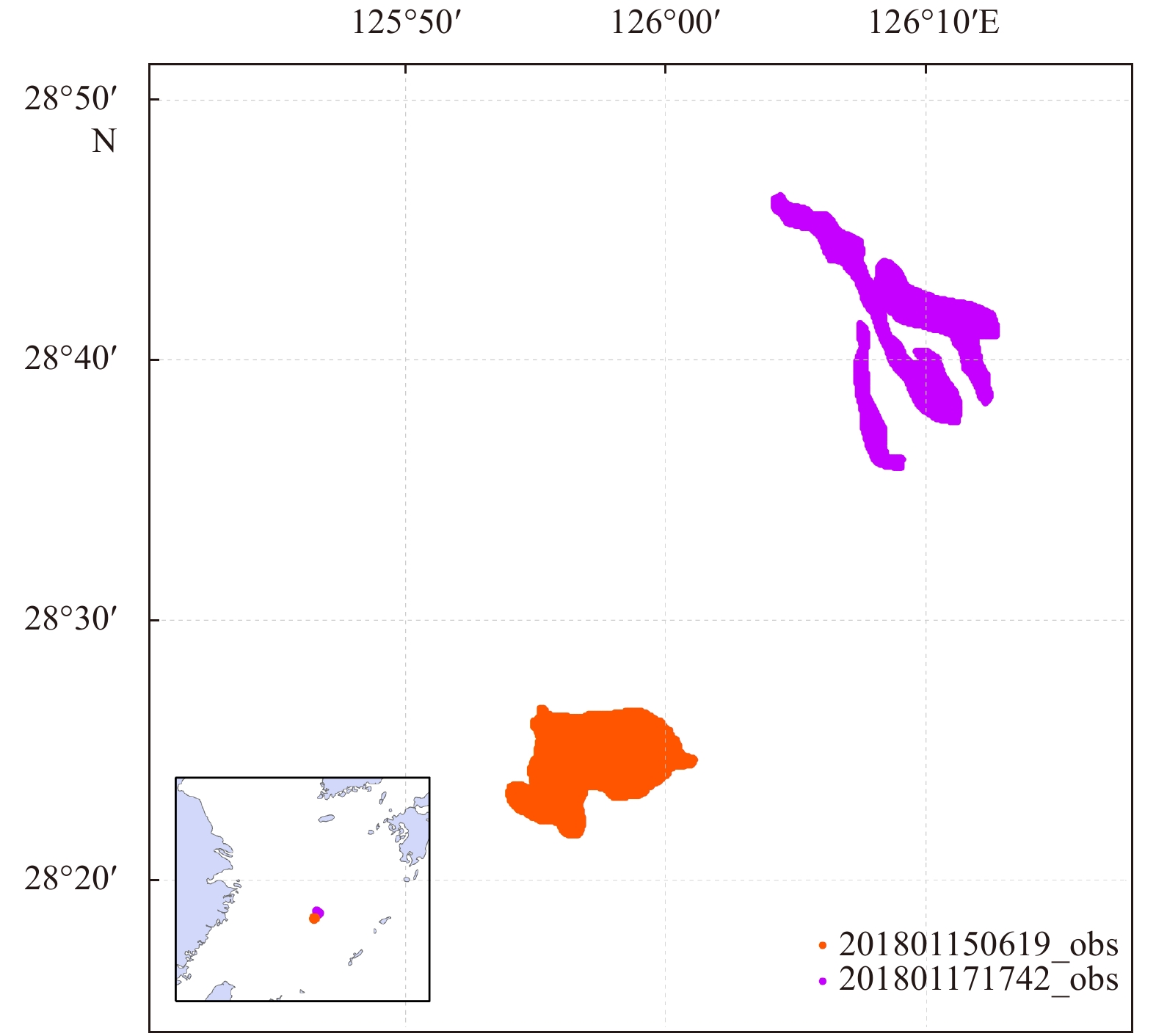
Oil slick images detected by satellite SAR (synthetic aperture radar) can provide initial input information for an oil spill model, including the time and location of an oil spill, as well as being used as a verification of the results of an oil spill model. In the Sanchi oil spill, two satellite remote sensing images were acquired from China’s National Satellite Ocean Application Service (NSOAS), which observed the distribution of oil on the sea surface (Fig. 1).

Figure  1.  The distribution on the sea surface of oil films observed by satellite. The orange represents oil observed at 6:19 on January 15, which is the initial information of oil spill. The purple represents oil observed at 17:42 on January 17, which is the verification information of the oil spill.

DownLoad: Full-Size Img PowerPoint

3. Model and data

3.1 Oil spill model

China’s National Marine Environmental Forecasting Center (NMEFC) has developed and uses its own 3-dimensional oil spill forecasting system since 2007 (Yang et al., 2017), which is based on oil particle tracking in a Lagrangian frame of reference and a random walk model.

In this study, a 2-dimensional oil spill model simplified from a 3-dimensional model was used, to simulate the transportation of heavy fuel oil on the sea surface. The model considered four factors: first, the heavy fuel oil has a longer lifetime on the sea surface than condensate (Pan et al., 2020); second, the satellite image only detects oil on the sea surface; third, Stokes drift will decrease rapidly with depth below the surface; fourth, oil will usually rise rapidly to the sea surface, close to the projection location of oil leak site on the sea surface.

In general, oil tracking by numerical models uses virtual particles. It is assumed that spilled oil is composed of a large number of particles with equal mass (Johansen, 1984, 1987; Elliott et al., 1986) and those particles are subject to wind, currents, waves, and turbulent diffusion. The velocity of oil particle is calculated as:

where $ {u}_{0} $, $ {v}_{0} $ are the horizontal velocities of the oil particle in x, y direction on the sea surface; $ {u}_{\rm{c} } $, $ {v}_{\rm{c}} $ are the horizontal velocities of current effected on oil particle, and are spatially interpolated at the oil position; $ {u}_{\rm{a}} $, $ {v}_{\rm{a}} $ are the wind velocities at 10 m above the sea surface; $ \alpha $, $ \beta $ are wind drift factor and drift angle, and $ \alpha $, $ \beta $ are taken as 0.02 and 0 in the paper according to the suggestion of Li (2013a); $ {u}_{\rm{w}} $, $ {v}_{\rm{w}} $ are the velocities of Stokes drift, and $ {u}' $, $ {v}' $ are turbulent diffusion.

where $ R $ is a random number in the interval between 0 and 1, $ {E}_{\mathrm{v}} $ is the turbulent coefficient, $ {c}' $ is the scaling coefficient, and Δt is time step in model.

3.2 Wind data

Li et al. (2013a, b) identified that wind is the major source of error in oil spill transport modeling. Previous studies (Pan et al., 2020; Li et al., 2019) have shown that the ECMWF (European Centre for Medium-Range Weather Forecasts) forecasted wind performs better in oil spill simulations. Therefore, the quality of different wind products did not be compared, but directly utilized the ECMWF forecasted wind as the oil spill model forcing. The medium-range forecasting products of ECMWF provided the wind forecast value at 10 m for the next 10 days with the 6 h and 9 km resolution in temporal and spatial, respectively.

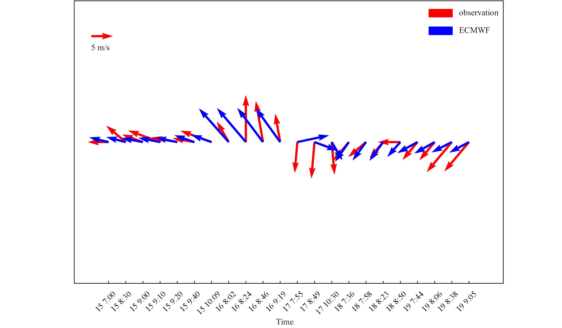
Wind observations from the cleaning ship around surface oil film, were used to validate the forecasted wind. Bilinear interpolation is used in space, and linear interpolation is used in time to compare the observed and ECMWF forecast wind (Figs 2 and 3). The mean absolute error (RAE) between the ECMWF forecast and the observations was 1.4 m/s in speed and 24.5° in direction. Generally, the forecasted wind was consistent with the observed recordings.

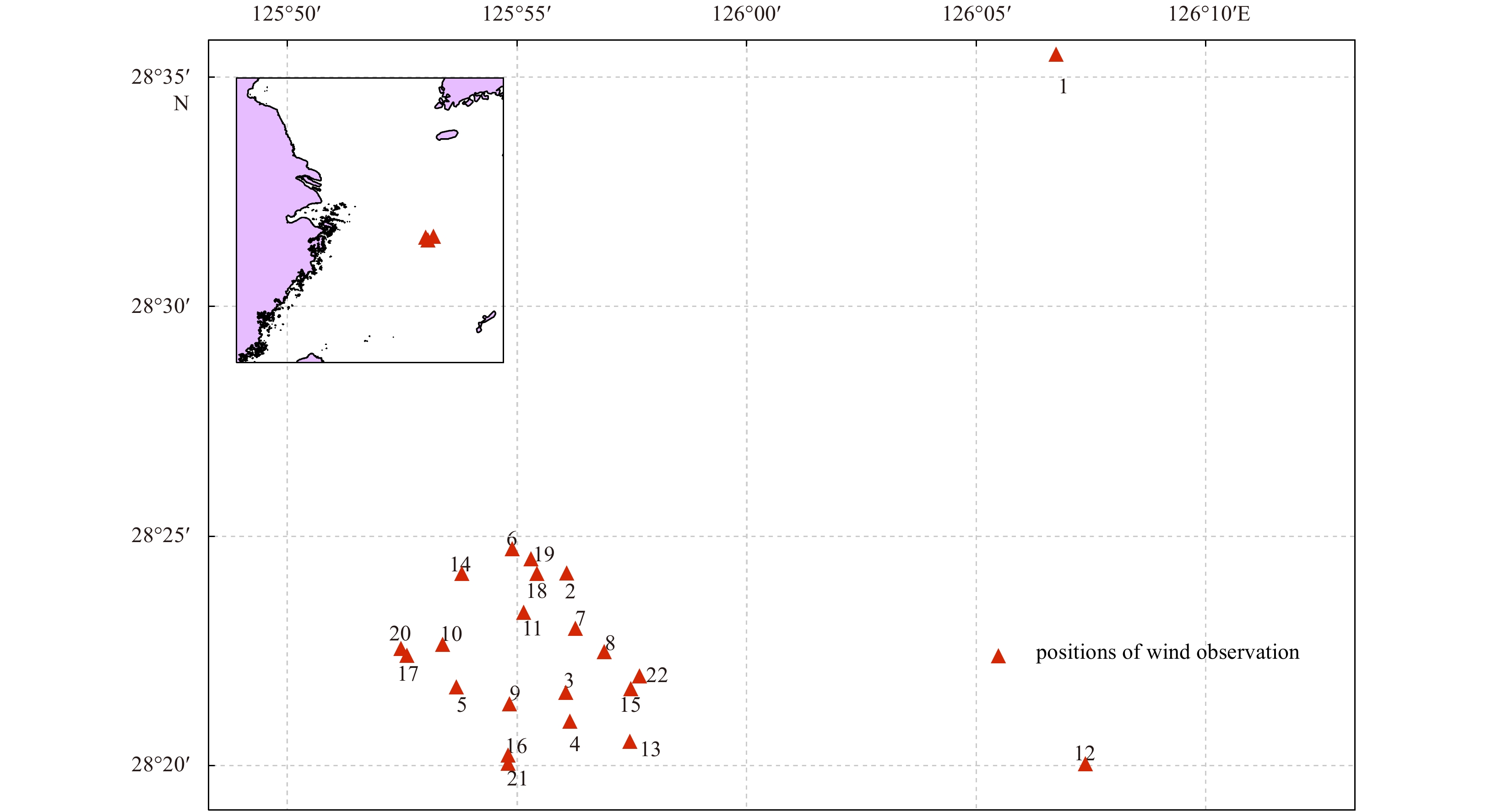
Figure  2.  The position of wind observations from the cleaning ship. Positions 1 to 22 correspond to the observation times in Fig. 3.

DownLoad: Full-Size Img PowerPoint

Figure  3.  The comparison of wind vector of ECMWF forecasting and observation.

DownLoad: Full-Size Img PowerPoint

3.3 Current data

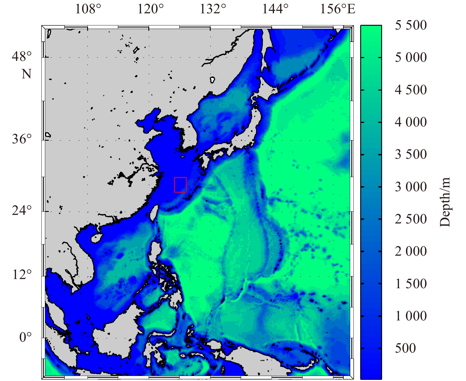
The operational Northwestern Pacific Ocean model (NWPM) is a regional model, which is based on the Regional Ocean Model System (ROMS), a free-surface, primitive equation ocean circulation model formulated using terrain-following coordinates, and run at NMEFC (Wang et al., 2016, 2017). It provided the next 120 h (every hour) forecasted sea surface currents, and temperature with the resolution of (1/20)°, extended from 8°S to 52°N and from 99°E to 160°E (Fig. 4).

Figure  4.  The region and topography of the northwestern Pacific Ocean. The red box is the computational domain of oil spill.

DownLoad: Full-Size Img PowerPoint

3.4 Stokes drift

Small particles, such as oil, plastic, are carried partly by the Stokes drift generated in the uppermost water layer in response to wind and waves (Isobe et al., 2014). However, the influence of Stokes drift is not often included in ocean reanalysis or forecasting products (Wang et al., 2017; Sakov and Sandery, 2015). In this study, two methods were used to calculate the velocity of the surface Stokes drift, the first was calculated from a wind-related formula which was based on a one-dimensional frequency spectrum, and the second was obtained from a wave model that was based on a two-dimensional spectrum.

3.4.1   Stokes based on one-dimensional frequency spectrum

Oil spill models are commonly driven by current and wind data that are easily available. The Stokes drift velocity is the function of wave and the significant wave height calculations using the JONSWAP wave spectrum parameterization. The Stokes drift velocity formula is as follows:

where $ k $ is wave number, $ \omega $ is wave angular frequency, and $ S\left(\omega \right) $ is wave spectra (JONSWAP Spectrum).

JONSWAP is measured by moderate winds and limited wind distances. JONSWAP spectrum is calculated as follows:

where $ \gamma $ is peak lift factor, which is between 1.5 and 6, $ \sigma $ is a factor of the shape of the wave, $ \alpha $ is a factor of wave energy, $ {\omega }_{\mathrm{m}} $ is the frequency of a wave crest, and $ g $ is acceleration of gravity.

$ \alpha $, $ \sigma $, $ {\omega }_{\mathrm{m}} $ satisfy the following formula:

In the above formula, $\widetilde {X}$ is the dimensionless zone length and described as follows:

where $ \widetilde X $ is wind distance, and $ {U}_{10} $ is the wind velocity at 10 m above the sea surface.

3.4.2   Stokes based on a two-dimensional spectrum

The second method of obtaining the Stokes drift velocity was from wave models, which were based on a two-dimensional spectrum. In this study, the CMEMS (Copernicus Marine Environment Monitoring Service) global ocean reanalysis wave system of Météo-France (WAVERYS) with a resolution of (1/5)°, provided analysis for the global ocean sea surface waves, which was applied to NMEFC’s oil spill model. The core of WAVERYS is based on the MFWAM (Meteo France Wave Model), a third generation wave model operated daily at Météo-France (Aouf et al., 2018). This product includes 3-hourly instantaneous fields of integrated wave parameters from the total spectrum (significant height, period, direction, Stokes drift, etc.). Stokes drift velocity in x- and y-directions can be downloaded from their website https://resources.marine.copernicus.eu/. The Stokes drift of domain is shown in Fig. 5.

Figure  5.  Stokes velocity at the start time of modeling. The color and arrows represent the values and direction of Stokes velocity, respectively.

DownLoad: Full-Size Img PowerPoint

In MFWAM the surface Stokes drift was defined by the following integral expression (ECMWF, 2020):

where $ \widehat{\boldsymbol{k}} $ is the unit vector in the direction of wave propagation, $ \theta $ is the direction in which the wave component is travelling, and $ E(\omega,\theta) $ is two-dimensional wave spectrum.

The integration is performed over all frequencies and directions.

4. Model setup and sensitivity experiments

Utilizing the Sanchi oil spill as the case model, the numerical simulations were carried out. The model assumes that 300 virtual oil particles were released instantaneously in the oil films area observed by satellite at 06:19 on January 15 (Fig. 1). The NMEFC-NWP’s sea surface current with a 1 h time step and WAVERYS’s Stokes drift with a 3 h time step were linearly interpolated to 10 min of a model time step. A total of 60 h from simulation start to end.

To evaluate the influence of Stokes drift in oil spill simulations, a series of sensitivity experiments were designed (Table 1). The sensitivity experiments were generally divided into three groups according to the different calculations of Stokes drift, with at least three experiments present per group. The first group EXP (experiment) 1–6 were driven by the same wind and current, but different wind-drift factors, ranging from 2%–3% (more suitable for NMEFC’s oil spill model), without considering the influence of Stokes drift. In the second group EXP 7–9, Stokes drift was calculated from a function of a one-dimensional frequency spectrum, here be defined as Method 1. In the third group, the value of Stokes drift was calculated from an analysis product of sea surface waves that was based on a two-dimensional spectrum and was considered as Method 2.

Table  1.  Sensitivity experiments

Group	No.	Wind	Current	Wind-drift factor/%	Stokes drift	Distance error/km
1	1	ECMWF	NMEFC-NWP	2	0	15.68
	2	ECMWF	NMEFC-NWP	2.5	0	12.88
	3	ECMWF	NMEFC-NWP	3	0	10.12
	4	ECMWF	NMEFC-NWP	4	0	6.24
	5	ECMWF	NMEFC-NWP	5	0	5.39
	6	ECMWF	NMEFC-NWP	6	0	8.72
2	7	ECMWF	NMEFC-NWP	3	Method 1	7.97
	8	ECMWF	NMEFC-NWP	4	Method 1	2.97
	9	ECMWF	NMEFC-NWP	5	Method 1	6.14
3	10	ECMWF	NMEFC-NWP	2	Method 2	8.13
	11	ECMWF	NMEFC-NWP	2.5	Method 2	1.03
	12	ECMWF	NMEFC-NWP	3	Method 2	3.03

 | Show Table

DownLoad: CSV

In this paper, distance error was used to judge the model results.

where $ R $ is earth radius, $ {DE}_{{\rm{MO}}} $ is distance error, $ {y}_{{\rm{M}}} $ is latitude of geometric center of model result, $ {y}_{{\rm{O}}} $ is latitude of geometric center of observation, $ {x}_{{\rm{M}}} $ is longitude of geometric center of model result, and $ {x}_{{\rm{O}}} $ is longitude of geometric center of observation.

5. Results

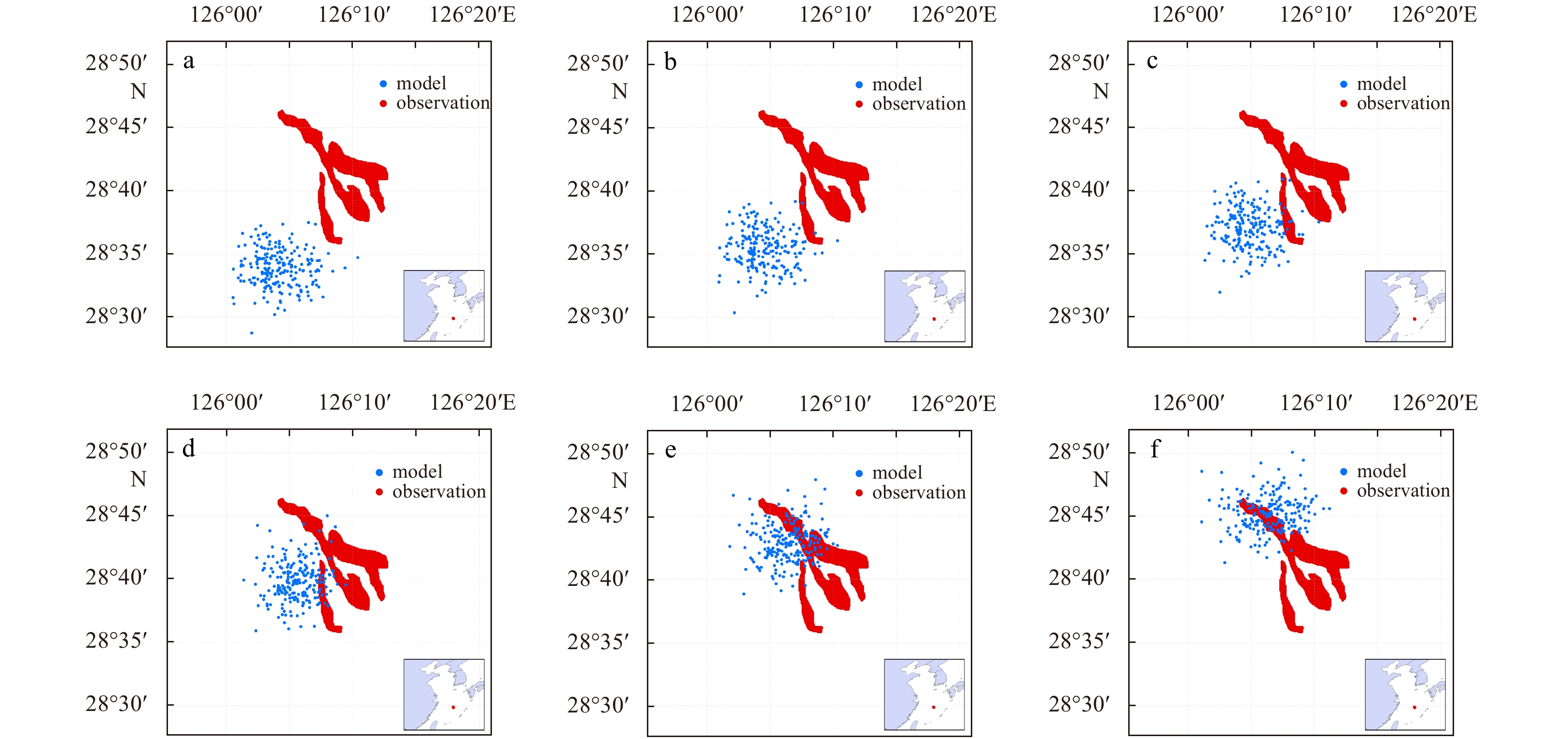
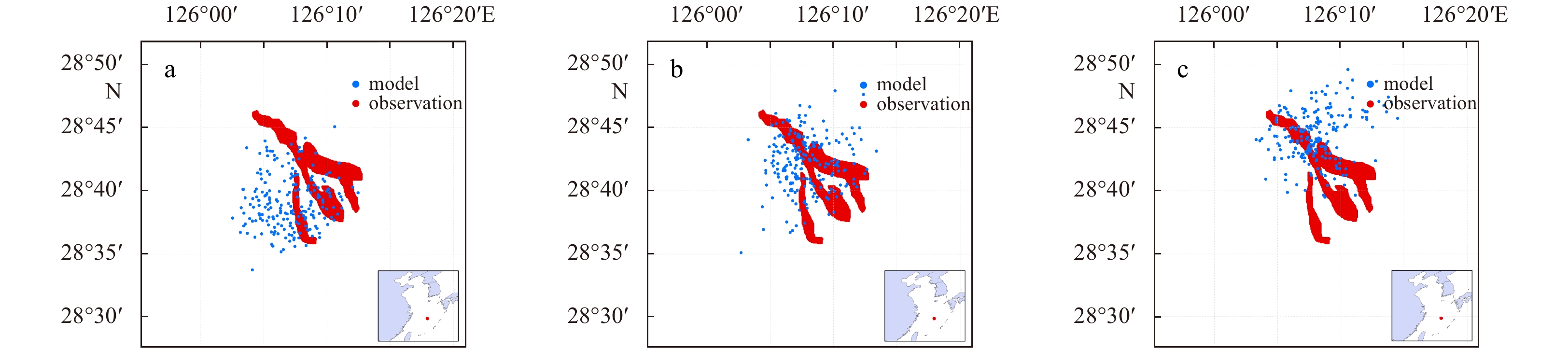
In the first group of experiments (Fig. 6), the oil particles drifted without considering the effect of Stokes drift. It can be seen from the three groups EXPs that the oil particles drift is farther if the wind drifts factor is larger. Given the suitable wind-drift factor of 2%–3%, none of the three experiments resulted in oil particles reaching the observation region (Figs 6a–c). After continuing to increase the wind drift factor by 4%–6%, some particles travelled to the northern area of the observation region (Figs 6d–f). The fifth experiment, with a wind drift factor of 5%, was the closest to the observation region in group 1 (Fig. 6e).

Figure  6.  The comparison of forecasting results and observations in group 1. a. Wind drift factor is 2%; b. wind drift factor is 2.5%; c. wind drift factor is 3%; d. wind drift factor is 4%; e. wind drift factor is 5%; f. wind drift factor is 6%.

DownLoad: Full-Size Img PowerPoint

In group 2, where the velocity of Stokes drift was a function of a one-dimensional frequency spectrum, the influences of different wind drift factor were also compared (Fig. 7). When the wind drift factor was 3%, one group of particles reached the observation area, while the other particles remained southwest of the observation area (Fig. 7b). After increasing the wind drift factor to 4%, most of the particles reached the observational area. If the wind drift factor continued to increase to 5%, the oil particles began to travel past the observational area and drift to the northeast (Fig. 7c).

Figure  7.  The comparison of forecasting results and observations in group 2. a. Wind drift factor is 3%; b. wind drift factor is 4%; c. wind drift factor is 5%.

DownLoad: Full-Size Img PowerPoint

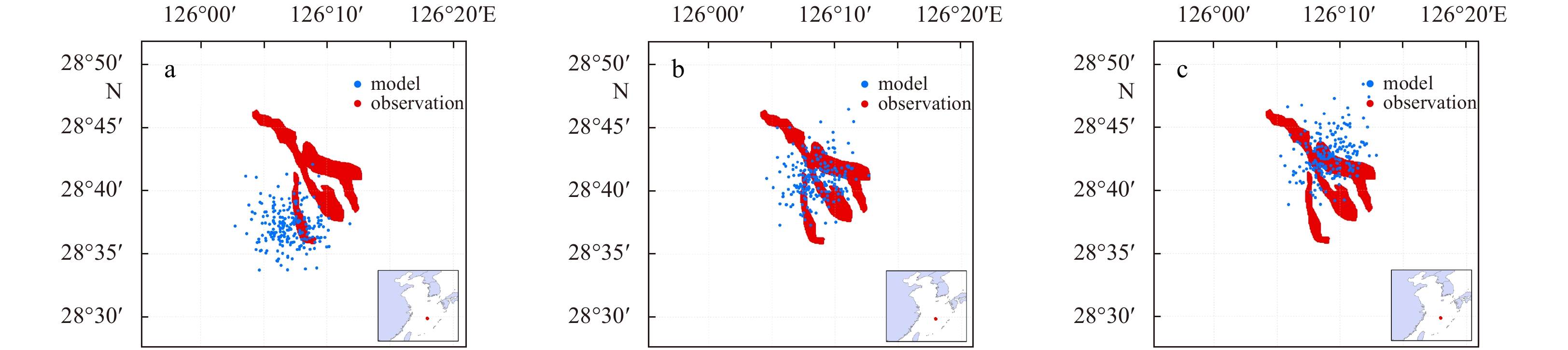
Considering the velocity of Stokes drift that based on a two-dimensional spectrum, the results of an oil spill are shown in Fig. 8. Driven by the 2% wind drift factor, one-third of the particles arrived at the observation area of oil (Fig. 8a). This was different from the previous two experiments, given that the results of simulation were partly consistent with the observations under the wind drift factor at 2%, and the increase in wind drift factor was reduced in this group. When the wind drift factor was increased to 2.5%, the majority of oil particles were located in the observation area. Any further increase in the wind drift factor results in oil particles travelling past the observation area to the northeast.

Figure  8.  The comparison of forecasting results and observations in group 3. a. Wind drift factor is 2%; b. wind drift factor is 2.5%; c. wind drift factor is 3%.

DownLoad: Full-Size Img PowerPoint

6. Discussion

By comparing the results of group 1 (excluding Stokes drift), to groups 2 and 3, the oil particles drifted noticeably farther after adding the velocity of Stokes drift when experiencing the same wind drift factor. For example, when the wind drift factor was set at 2%, the oil particles were closer to the observation area when calculated under the influence of Stokes drift (Figs 6a and 8a). This shows that the role of Stokes was positively related to the wind. In the case of the 3% wind drift factor (EXP 3, 7 and 12) which is recommended by most oil models, the effect of Stokes can bring the particles closer to the observation area.

In the first group of experiments without the influence of Stokes drift, the closest simulation result was from the wind forcing factor of 5%, although the drift distance error was 5.39 km. In the second group of experiments, the optimal result was produced by experiment 8 with the wind drift factor of 4%, whereby the drift distance error was 2.97 km. In the third group of experiments, the most consistent result with the observational data was experiment 11, with the smallest drift distance error of 1.03 km, and a wind drift factor of 2.5%. During the oil spill simulation, a lower wind drift factor was required when considering the influence of Stokes drift, reducing from 5% to 2.5%. Therefore, the Stokes drift caused by waves, is of the order of 2.5% of the wind speed.

Comparing group 1 with groups 2 and 3, it can be seen that the oil spill simulation under the influence of Stokes drift (groups 2 and 3) was considerably better than with group 1. However, the drift distance of group 3 was farther from the initial position than other groups under the same wind drift factor, so a smaller wind drift was required in group 3 experiments. If the velocity of Stokes drift obtained from the first method was used in the oil spill model, the recommended wind drift factor would be approximately 0.04; while if the velocity of Stokes drift was derived from the wave model, the recommended wind drift factor would be approximately 0.025.

It can be seen from group 2 and group 3 that the simulation experiment using a one-dimensional wave spectrum (Method 1) required stronger wind information to make the particles reach the best position. The two-dimensional wave spectrum (E(w,θ)=S(w)·D(θ)) is the one-dimensional spectrum S(w) multiplied by the D(θ) direction distribution function (Barstow et al., 2005). The θ is a function related to wind, so less wind is required when calculating with the two-dimensional wave spectrum. The one-dimensional wave spectrum is simplified from two-dimensional wave spectrum, and its direction was mainly dominated by wind. In fact, the energy of the waves was related to the direction. Therefore, the Stokes drift velocity calculated by the two-dimensional wave spectrum was more accurate than the one-dimensional wave spectrum, but the calculation cost is higher.

7. Conclusions

In this analysis, in order to determine the influence of Stokes drift in forecasting oil spills, three groups of experiments were designed to simulate the Sanchi oil spill. Two methods were utilized to quantify the velocity of Stokes drift, the first was calculated from a one-dimensional frequency spectrum, the second was obtained from the wave model based upon a two-dimensional spectrum. The conclusions are as follows:

If the wind drift factor of 3% (suitable for NMEFC’s oil spill model) is used without considering the influence of Stokes drifts, the virtual oil particles in a model could not reach the observed spill area, distorting the simulation result. Even if the wind drift factor was increased to 5%, the forecast is not as ideal as one that considered the influence of Stokes drift. Therefore, the velocity of Stokes drift is related to the wind, but it is not a linear relationship. It cannot therefore simply be replaced by increasing the wind drift factor, which could induce errors in the resulting simulation. The Stokes drift velocity of the linearized wind drift factor will result in the drift of the surface oil particles be dominated by wind, which ignores the deviation between the displacement direction caused by the motion of the waves and the wind direction. After considering the Stokes drift, the angular deviation was reduced between simulation and observation, thereby reducing the distance error (Figs 5 and 8) and benefitting the oil spill simulation.

The influence of Stokes drift can be ignored in the 1–2 day short-term forecast. Due to the viscous tension of the oil film surface, the sea surface is quite smooth and thereby weakens the Stokes effect (Mu et al., 2011). However, for medium and long-term simulations longer than two days or more, Stokes drift is a factor that cannot be ignored, and its magnitude can reach about 2% of the wind speed.

The Stokes drift velocity obtained from the two-dimensional wave spectrum was more accurate, but its calculation requires integration of frequency and direction, so the calculation efficiency was lower. Therefore, it is optimal to use the Stokes drift velocity from the wave mode when it is available, otherwise, it can be calculated from one-dimensional frequency spectrum. However, as calculating Stokes effect from the wind occurs concurrently with the oil spill simulation, the model runs slightly slower than the Stokes drift was obtained from wave models directly.