College of Marine Sciences, Shanghai Ocean University, Shanghai 201306, China
2.
Project Management Office of China National Scientific Seafloor Observatory, Tongji University, Shanghai 200092, China
Funds:
The National Natural Science Foundation of China under contract No. 4210060098; the Foundation of Key Laboratory of Sustainable Exploitation of Oceanic Fisheries Resources under contract No. A1-2006-21-200201.
The current lack of high-precision information on subsurface seawater is a constraint in fishery research. Based on Argo temperature and salinity profiles, this study applied the gradient-dependent optimal interpolation to reconstruct daily subsurface oceanic environmental information according to fishery dates and locations. The relationship between subsurface information and matching yellowfin tuna (YFT) in the western and central Pacific Ocean (WCPO) was examined using catch data from January 1, 2008 to August 31, 2017. The seawater temperature and salinity results showed differences of less than ±0.5°C and ±0.01 compared with the truth observations respectively. Statistical analysis revealed that the most suitable temperature for YFT fishery was 28–29°C at the near-surface. The most suitable salinity range for YFT fishery was 34.5–36.0 at depths shallower than 300 m. The suitable upper and lower bounds on the depths of the thermocline were 90–100 m and 300–350 m, respectively. The thermocline characteristics were prominent, with a mean temperature gradient exceeding 0.08°C/m. These results indicate that the profiles constructed by gradient-dependent optimal interpolation were more accurate than those of the nearest profiles adopted.
Analyzing the environmental characteristics of fish activity is important in fishery oceanography. The basic properties of seawater, such as temperature and salinity, have important effects on fish behavior: different types of fish have different temperature and salinity requirements (Song and Wu, 2011; Lan et al., 2017). In the past decades, sea surface observation data were obtained by satellite sensors at various spatial and temporal scales, which is helpful for fishery research in the open ocean (Laurs and Fiedler, 1985; Fiúza, 1990; Kluger et al., 2016; Lan et al., 2017). However, many important processes and structures associated with fishery resource distribution occur below the surface or at greater depths. As a major component of the ocean observation system, the increasing Argo array has allowed, for the first time, a near-global sampling of the upper 2 000 m of ice-free oceans with relatively small bias since 2005 (Roemmich and Gilson, 2009; Johnson et al., 2015; Liu et al., 2020). The obtained subsurface environmental data containing multiple variables and can be used to better understand the relationships between oceanic environments and fishing conditions. However, the spatial–temporal mismatch between fishery and environment data means that the latter cannot be used effectively in fishery research. Presently, the integration of available environmental data sources into fishery data is a challenging but urgent task in fisheries oceanography.
Tuna species are critical commercial open-ocean fish and are of great ecological importance. For example, the yellowfin tuna (YFT) can swim at high speeds and exhibit deep-diving behavior (diving to over 500 m) (Schaefer et al., 2007, 2009). They dive into deep depths for food and spend about 30% of the daytime below the thermocline. It is believed that the long-distance vertical movement of the YFT may weaken the correlation between the YFT catch rate and sea-surface temperature (Zagaglia et al., 2004; Schaefer et al., 2011, 2014). Many studies have indicated that the longline catch per unit effort of the YFT had a closer relationship with the subsurface water temperature rather than the surface water temperature. Therefore, the vertical temperature structure, especially the thermocline distribution, is a vital factor in tuna fisheries (Langley et al., 2009; Lan et al., 2011; Yang et al., 2015). Nevertheless, research on the relationship between oceanic interior characteristics and fishery activities is rare because of the lack of synchronous environmental observations with catch data. Some studies rely on inversion models, climate-gridded products, or finding the nearest synchronous observation (Song and Wu, 2011; Klemas and Yan, 2014; Yang et al., 2015). Subsurface data retrieved from satellites or climate products have the problem of spatial–temporal mismatch. When the distance is significant, the nearest synchronous observation may describe the environment imprecisely or unilaterally. It is necessary to develop an approach to solve this problem.
Optimal interpolation (OI) is an objective analysis method proposed by Gandin (1963). OI equations can be easily derived as a variation problem to find a vector of estimates that minimizes the total error variance of the field being estimated (Wikle and Berliner, 2007). The estimator is unbiased and linear between the observations and the first estimate (a priori estimation) of the field. It has been widely used to calculate the gridded analysis data for ocean numerical models (Bonanno et al., 2019; Burgess and Webster, 1980; De Feis et al., 2020). Zhang et al. (2013) proposed the gradient-dependent correlation scale method, which uses the horizontal gradient change of oceanographic elements to estimate the correlation scales in the OI. This scheme, named gradient-dependent OI in the following, effectively extracted shorter wavelength information in zones with a large gradient (Zhang et al., 2015). It provides a new perspective for constructing real-time environmental information of fishing sites using a point-to-point method. The optimal weighted average is expected to provide results close to real observations. Then, we provide a data basis for better study of the fish living environment.
In this respect, this study applies the gradient-dependent OI to obtain high-resolution subsurface data from the Argo array according to YFT fishery dates and locations in the western and central Pacific Ocean (WCPO). The results were used to determine the most suitable environmental conditions for YFT fishing. The fishery and Argo observations and the principle of the method are described in Section 2. In Section 3, we verify the results and apply them to validate the relationship between fish activities and the subsurface seawater environment. We discussed the suitable temperature and salinity vertical distribution for YFT in Section 4. Finally, in Section 5, we present our conclusions.
2.
Materials and methods
2.1
Fishery and environment data
Daily fishery data from the WCPO purse seiners were obtained between January 1, 2008 and August 31, 2017 from 14 ocean-going fishing vessels (Jinhui 1, 2, 3, 6, 7, 8, 9, 18, and 58, Pohnpei1, LOJET, LOMETO, LOMALO, and MAJURO1) of the Shanghai Kaichuang Fishery Co., Ltd. (SKFC). These data included the date, longitude, latitude, operation type (free-swimming and fish-aggregating device used), ship name, daily catch per ship, and other production information. The amount of free-swimming was small, and we selected the fishery data of the fish aggregating device (FAD) used only (Fig.1a). There were 6354 fishery points used in this study. These fishing vessels have similar fishing capacities. Therefore, this study ignored the influence of ship properties on fishery catch data. We adopted the daily output per ship as the catch as the measure of the resource abundance.
Figure
1.
Location of YFT fishery points and the available Argo observations. a. The YFT fishing locations in the WCPO and the locations of fishing locations and Argo profiles during August 2017; b. the frequency statistic of observation number surrounding each fishing point.
Two categories of environmental data were collected in this study: Argo profiles and WOA18 gridded data. The former were derived from the China Argo Real-Time-Data Center (ftp://ftp.argo.org.cn/pub/ARGO/global/). These include temperature, salinity, and pressure, which are processed in real-time and delayed-mode quality control (Tong et al., 2003; Liu et al., 2006). We collected Argo observations for the same period as the YFT catch data in the WCPO. A radial distance of 500 km was set to ensure that more than five Argo temperature and salinity profiles were obtained at every fishery point each day. Only profiles located within the specified range were used to establish subsurface environmental information for fishery points at depths between 5 m and 1500 m. A total of 62726 Argo profiles surround the 6354 fishery points. Figure 1a displays the locations of fishery points in August 2017 and their corresponding Argo profiles within the effective radius. The frequency statistics of the available Argo observations surrounding every fishery point are shown in Fig. 1b. All fishery points have more than 10 and sometimes as many as 35 environmental profiles within the specified range. Most fishery points have 15–23 available profiles. The World Ocean Atlas 2018 (WOA18) gridded data were used to calculate the horizontal gradients and provide the first guess field via bilinear interpolation at each fishery point. Two gridded datasets, longitude, latitude, pressure, temperature, and salinity were downloaded from the Ocean Climate Laboratory of NODC (https://www.nodc.noaa.gov/OC5/woa18/). These data have a pixel resolution of (1/4)° and span the area from 30°S to 30°N and 120°E to 140°W.
2.2
Gradient-dependent OI
The purpose of the scheme was to obtain an optimal analysis value for the goat point based on least squares theory. The analysis results at the fishery point was used as the background value plus the innovation value weighted by the optimal weights. As for the fishery point influenced by M observations, the standard analysis equation is given by Eq. (1). A critical part of the scheme is to estimate the optimal weights. According to the minimum variance theory, the optimal weight can be determined by solving Eq. (2) (Kalnay, 2003):
where $ v_i^a $ is the analysis value and $ v $ can be any environmental variable, such as temperature or salinity. The first estimate $ v_i^b $ was given by the WOA18 monthly data via bilinear interpolation. The subscript i denotes the number of fishery sampling points, and j and k denote the number of available Argo profile sites. For observational increments, $ \delta y_j^o{{ = }}y_j^o{{ - }}H(v_j^b) $, the observational operator H converted the background field into the first guesses of the observation $ y_j^o $. In this study, a radial distance was set to ensure that only the Argo profiles located within a specified range surrounding each fishery point were counted. Each increment has an optimal weight $ {w_{ik}} $ associated with the background error correlation, $ {\mu _{jk}} $ and $ {\mu _{ik}} $. where $ {\mu _{jk}} $, $ {\mu _{ik}} $ are the correlations between the background errors at the two observational points, j and k, and at the fishery and observation points i and k, respectively. $ \eta $ is the mean square of the relative observation errors compared with the background errors, which was frequently “tuned” to vary the weights of the observation. We used the value of $ \eta {{ = 0}}{{.25}} $ for the Pacific Ocean in this study (Zhang et al., 2015). The correlations are usually assumed to follow a Gaussian exponential function (Zhang et al., 2013):
where x and y are the longitude and latitude, respectively, and $ {L_\phi }/G $ depend on the Rossby radius of deformation and the horizontal gradient changes, which define the background error correlation scale. $ {L_\phi } $ is the correlation scale that can be obtained from the scale parameter multiplied by the cosine function of the latitude ($ \phi $) at fishery sampling point i. The radial distance was set to 500 km when constructing high-resolution profiles to ensure that a sufficient number of observations were considered. The parameter G, calculated using the WOA18 climatological data, is associated with the horizontal gradient (s) at location i. It contains a zonal component ($ G_x $) and a meridional component ($ G_y $). The Gaussian functions presented in Eqs (3–5) provide anisotropic background error correlations at each fishery point.
3.
Results
According to the algorithm described in Eqs (1–5), we obtained 6354 temperature and salinity profiles based on Argo observations. Each profile was obtained on the same time (day) and location as the YFT fishery data from January 1, 2008 to August 31, 2017, in the WCPO. The vertical depths (5–1500 m) were divided into unequally spaced 24 layers.
3.1
Verification of the results
We randomly selected 30 Argo T/S profiles as the “true” observations and constructed the analysis profiles according to the Argo observation locations using the gradient-dependent OI shown in Section 2.2. The true observations at each location were not included when we constructed the analysis profiles using the Argo observation profiles located within the specified range. These analysis profiles were then used to verify the algorithm by comparing them with the corresponding “true” observations. The verification was carried by calculating the root mean square errors (RMSEs) and differences between analysis and “true” observations. The RMSEs of analysis results and those of nearest profiles at the depth range of 5 m to 1 500 m were shown in Fig. 2. Figure 3 displays the temperature and salinity differences between analysis results and “true” observations at depths of 5 m to 500 m.
Figure
2.
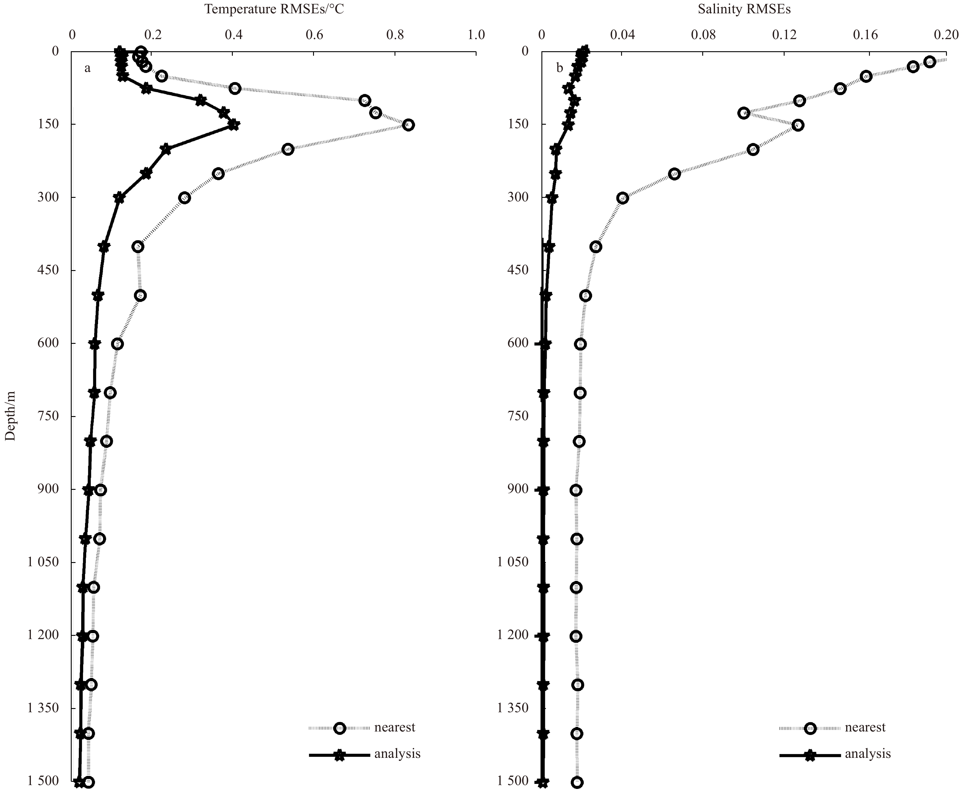
Root mean square errors (RMSEs) of 30 sample points from the analysis results (indicated by dots) and nearest profiles (indicated by circles) at a depth range of 5 m to 1500 m.
Figure
3.
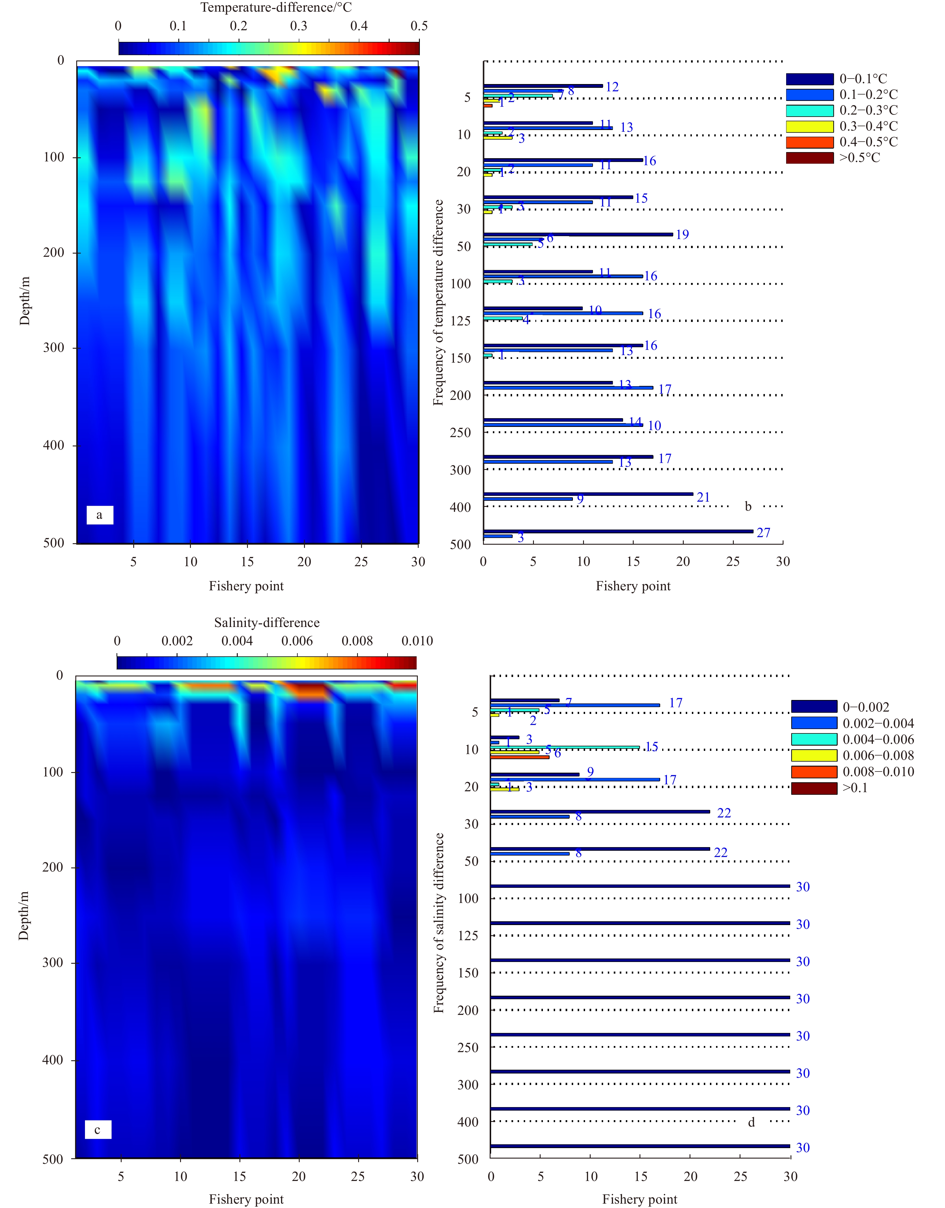
Temperature and salinity differences between 5 m to 500 m at each fishery point. a and c show the vertical difference distribution, whereas b and d are the difference frequency at each depth.
It can be seen that both temperature and salinity have larger RMSEs and differences at the upper depth than at the deep depth. The temperature differences were no more than 0.50°C and salinity differences were less than 0.01 above 500 m. Figures 3a and c indicate that the differences were near zero in the middle and deep layers. The maximum temperature RMSE is approximately 0.4°C. If the nearest temperature profiles are adopted, the corresponding RMSEs exceed 0.4°C at depths of 50 m to 300 m, which are the principal activity layers of YFT (Fig. 2a). As for the salinity RMSE (Fig. 2b), the difference was more significant. The salinity RMSEs of the analysis results present a value of less than 0.02 at a depth of 5–1500 m. At the nearest profiles, the salinity RMSEs are all larger than 0.04 above 300 m.
In other words, the analysis results were very close to the observations. Near the surface, the temperature and salinity differences were relatively significant. There were one-third profiles whose temperature differences are in 0.4–0.5°C at a depth of 5 m (Fig. 3b). At a depth of 10 m, 11 profiles in 30 had salinity differences of 0.006–0.01(Fig. 3d). The lack of surface observations in most Argo profiles made the true values scarce at 5 m, and the accuracy was lower. The salinity observations with more significant variances because of the salinity sensor drift at the near-surface would influence the accuracy of the analysis. However, most temperature and salinity differences at depths greater than 150 m were less than 0.2°C and 0.002, respectively. At depths deeper than 300 m, temperature RMSEs are less than 0.1°C, and salinity RMSEs are close to 0 for the analysis results. The nearest RMSEs are large, with a maximum RMSE of approximately 0.9°C for temperature and 0.17 for salinity, as shown in Fig. 2.
3.2
Application and analysis
The temperature and salinity profiles of 6354 constructed using Eqs (1–5) were applied to discuss the relationship between the YFT catch data and several oceanic environmental factors, including temperature, thermocline, and salinity, using frequency statistics and contrastive analysis. Most of the YFT catch values corresponding to these profiles were concentrated in 1–50 t. To give the general vertical characteristics clearly, we interpolated the temperature and salinity of each water layer to YFT catch values of 1−50 t. The temperature and salinity sections with the change in catch are displayed in Figs 4 and 5. The YFT suitable temperature and salinity were statistically significant at 5 m, 150 m, and 300 m, as shown in Fig. 6. Finally, the relationship between the thermocline parameters and YFT catch is shown in Fig. 7 and Table 1.
Figure
4.
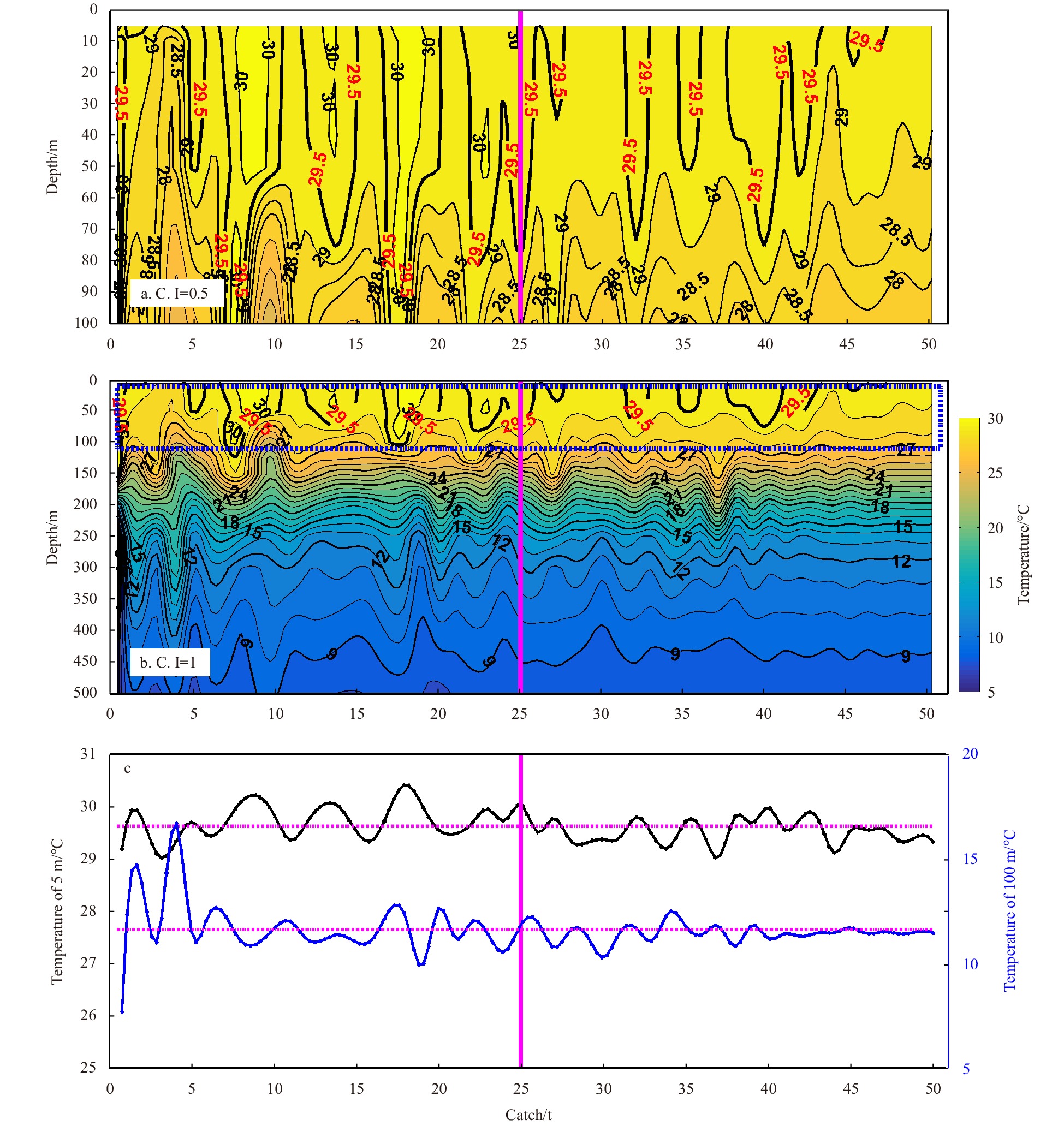
Temperature section at the depth range from 5 m to 100 m (a), 5 m to 500 m (b), and temperature curves at 5 m and 100 m (c) for different catch. The temperatures at every water layer were interpolated to the catch sequence. C. I indicates the contour intervals.
Figure
5.
Salinity section at the depth range from 5 m to 100 m (a), 5 m to 500 m (b), and salinity curves at 5 m and 150 m (c) for different catch. The salinities at every water layer were interpolated to the catch sequence. C. I indicates the contour intervals.
Figure
6.
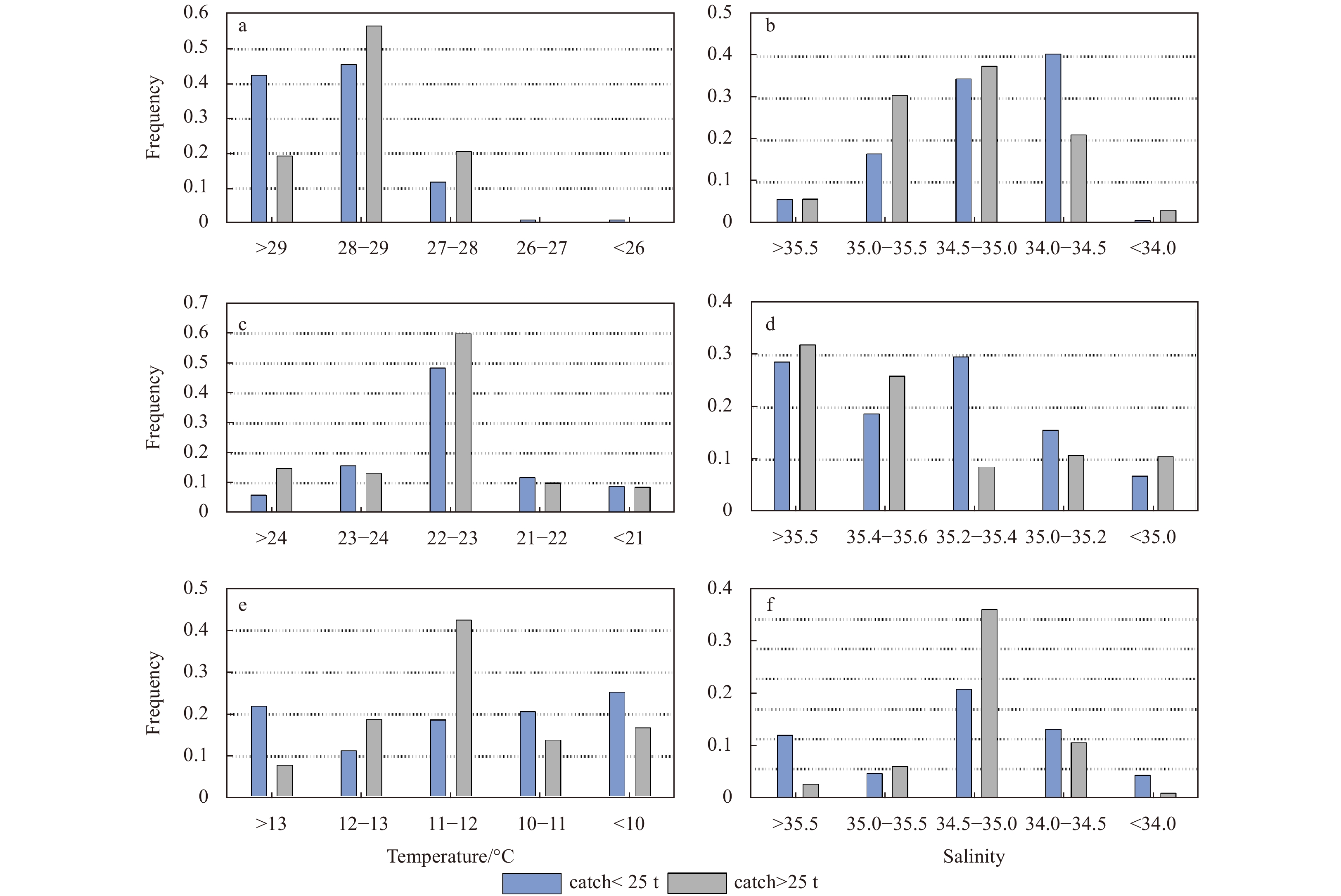
The statistic of suitable temperature and salinity for YFT corresponding different catch group. Temperature at 5 m, 150 m, and 300 m are indicated by a, c, and e, respectively. Salinity at 5 m, 150 m and 300 m are indicated by b, d, and f, respectively.
Figure
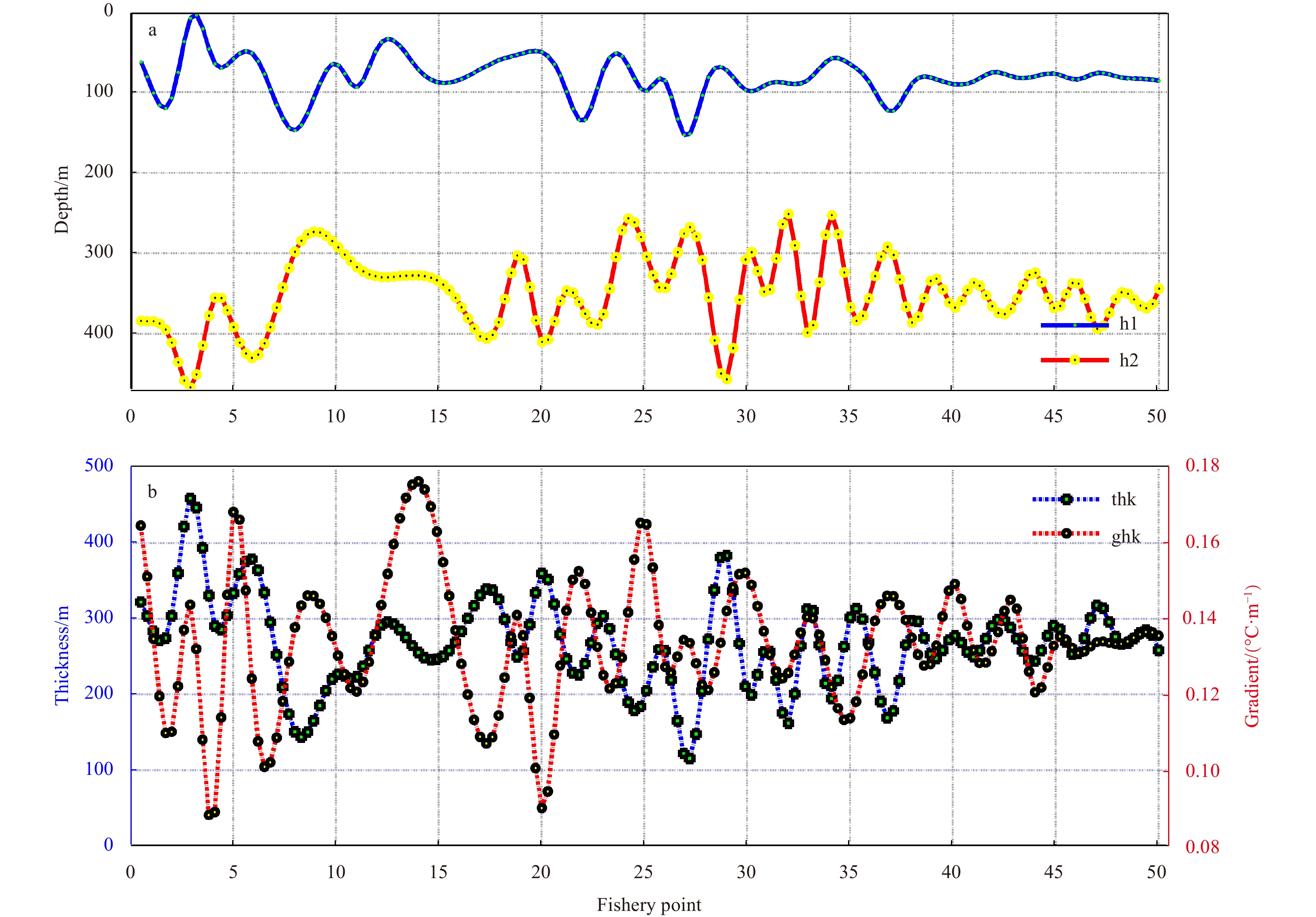
7.
Statistics for the thermocline variable matching each fishery point. a. The upper bound depth (indicated by h1) and the deeper bound depth (indicated by h2); b. the thermocline thickness (represented by thk) and thermocline strength represented by temperature gradient (indicated by gth).
Table
1.
Thermocline parameters for different catch (t) groups
<10 t
10−20 t
20−30 t
>30 t
h1/m
80−90
80−90
90−100
90−100
h2/m
350−400
350−400
350−400
300−350
thk/m
350−360
260−270
280−290
240−250
gth/(°C·m−1)
0.14−0.15
0.14−0.15
0.12−0.13
0.12−0.13
Note: The upper and deeper bound depth of the thermocline are represented by h1 and h2, respectively. Thk and gth indicate the thickness and gradient representing strength of the thermocline, respectively.
Figure 4b shows the general characteristics of the temperature distribution corresponding to different catches. At the fishery ground, the near-surface temperature was approximately 30°C. The temperature remained high (>27°C) up to a depth of 100 m. At a depth of 300 m, the temperature decreased significantly to 12°C. There was an evident thermocline corresponding to each catch value. When the catches were larger than 25 t, the temperature isopleths tended to be smooth. In contrast, the temperature fluctuated greatly with the catch change when the catch was small. The vertical temperature characteristics at the upper mixed layer (<100 m) are clearly displayed in Fig. 4a. It can be seen that many fishery points with lower catches had surface temperature values of 30°C at depths lower than 50 m and had temperature values of 28°C at depths of 50–100 m. At the fishery points with higher catches, their temperature was concentrated in the range of 28.5–29.5°C at depths of 5–100 m. The temperature curves shown in Fig. 4c clearly demonstrate the similar trends: (1) when the catches were higher (>25 t), the temperatures tended to be stable. Otherwise, the temperatures had large fluctuations at the YFT fishery points with lower catches. (2) At the near-surface, the temperatures of the fisher points with higher catches were slightly colder than those with a lower catch. (3) At all the fishery points, the vertical temperature change had a value of approximately 17°C at a depth of 5–300 m.
Figure 5 shows that the relationships between the YFT catch weights and seawater salinities had similar characteristics with temperature. Overall, the salinities presented high values of 35–36 at depths of 50–300 m (Fig. 5b). The near-surface salinity was approximately 34.5–35.5. Most salinities derived from higher catches (>25 t) were 34.5–35 at depths lower than 50 m. At the fishery points with lower catches, the near-surface salinities were concentrated in 34–35 (Fig. 5a) with salinity values near 35.5 at a depth of 150 m (Fig. 5c). When the catches were higher than 25 t, the salinity differences between the depths of 5 m and 150 m were less than 0.5. The vertical salinity change was smaller than that in the lower catch fishery points.
According to their weights, the YFT catches (daily output per ship) were divided into two groups: higher catch (>25 t) and lower catch (<25 t). Three representative layers (5 m, 150 m, and 300 m) were selected, and five parts were divided at each depth according to the temperature and salinity scale. Figure 6 displays the statistical results for suitable temperature and salinity for the YFT.
At the near-surface (<5 m), the suitable temperatures and salinity were 28–29°C and 34.5–35.0, respectively (see Figs 6a and b). The higher catches had smaller variations, and the lower catches had a large number of higher temperatures (> 30°C) and lower temperatures (<27°C). When the salinities were in the range of 35.0–35.5, the catches increased. However, the catches were lower with a salinity larger than 35.5 or smaller than 34.0. Suitable temperatures were 22–23°C at a depth of 150 m. This can be represented by both catch groups (Fig. 6c). Figure 6d shows that the suable salinities had a larger value of exceeding 35.6 at a depth of 150 m. When the salinities were between 35.4 and 35.6, the YFT were frequently active. At a depth of 300 m, the most suitable temperatures and salinities were 11–12°C and 34.5–35.0, respectively, just as shown in Figs 6e and f.
Thermoclines can be clearly observed in the upper ocean where the YFT migrates mainly. The thermocline, or the vertical temperature gradient, is an important factor influencing the YFT activities. Figure 7 shows the characteristics of the thermocline parameters corresponding to different catchments. The depth and strength of the thermocline were calculated using the maximum angle method (Chu and Fan, 2011). Here, we considered only the seasonal thermocline that existed in the top layer. The thermocline parameters were obtained first according to the Argo temperature profiles surrounding each fishery point. These parameters were then merged with the fishery points using the method described in Section 2.2. The thermocline parameters mainly included the upper bound depth (indicated by h1 in Fig. 7), the deeper bound depth (indicated by h2 in Fig. 7), and the temperature gradient that indicates the thermocline strength (indicated in the gth panel in Fig. 7). The thermocline thickness is represented by symbol thk.
Combined with Fig. 1, these fishery points were primarily located in the tropical western Pacific. The location of the thermocline was evident. Figure 7a shows that most of the upper bounds of the thermocline (h1) are 50–150 m. At points whose catches exceeded 25 t, the upper bound of the thermocline was approximately 100 m, which was deeper than that of the lower catch points. The deeper bound depth of the thermocline (h2) was between 250 m and 450 m. Most of the large catch points had a value of 300–400 m. The mean thermocline thickness was approximately 250 m at most fishery points. Fishery catches were lower when the thermocline thickness exceeded 300 m. As can be seen in Fig. 7b, the stronger the thermocline, the lower the catch. For the higher catch fishery points, most of them had temperature gradients (gth) of 0.12–0.15°C/m. For the fishery points with catches lower than 25 t, their corresponding temperature gradients (gth) were very large (>0.16°C/m) or very small (< 0.10°C/m). The temperature gradients of the thermocline were larger than 0.08°C/m at all of the fishery points.
Based on their weight, YFT catches were divided into four groups: < 10 t, 10–20 t, 20–30 t, and > 30 t. In Table 1, matching the four catch clusters (< 10 t, 10–20 t, 20–30 t, and > 30 t), the thermocline parameter ranges with the largest proportion are given. The h1, h2, thk, and gth results were given by statistics with intervals of 10 m, 50 m, 10 m, and 0.01°C/m, respectively. The table shows that the suitable upper (h1) and deeper bound depths of the thermocline (h2) were 90–100 m and 300–350 m, respectively. The corresponding suitable thickness was 240–250 m. The larger the thickness and gradient, the smaller the catches became. The most suitable temperature gradients for YFT were 0.12–0.13°C/m.
4.
Discussions
4.1
YFT and vertical T/S distribution
The YFT is a warm-water fish that needs a specific water temperature to inhabit and spawn. Studies have shown that the highest yield of YFT comes from areas where the surface temperature is approximately 29°C (Wang et al., 2014). The statistical results indicated that the most suitable temperatures and salinities for the YFT were 28–29°C at 5 m. Most fishery points with high catch values had temperature values of 29–29.5°C. When the near-surface temperatures were above 30°C or below 28°C, there were few catches. The vertical temperature decreased with increasing depth. The temperature was reduced to 22–23°C at depths of 150 m, where the YFT spent 5% of their time staying in the water layer. The temperature difference between the surface and 150 m was approximately 8°C. This is consistent with previous research results (Schaefer et al., 2007; Weng et al., 2009).
Salinity is not as critical as temperature. The suitable near-surface salinities were found to be 34.5–35.0. The higher the catch, the smaller the change in the vertical salinity. These conclusions are similar to those obtained in previous studies (Song and Wu, 2011; Yang et al., 2015). Most of the time, YFT lived in the warm water layer below 100 m and migrated to food in the upper ocean. The tolerance time of YFT to environmental changes is limited. They were more suitable for less vertical temperature and salinity changes, as shown in this study.
4.2
YFT and thermocline
The YFT can break through the temperature thermocline and enter the deep water layers, even deeper than 1000 m (Schaefer et al., 2011). However, it was also pointed out that the purpose of YFT frequently entering deep water was foraging. Thermocline may influence the diurnal vertical distribution of the YFT by affecting the diurnal vertical distribution of food organisms. Most of the time, the YFT lived in water layers lower than 100 m but rarely below 10 m in the western and central Pacific Ocean (Leroy et al., 2007). Compared with sea surface environmental information, the thermocline had a more significant effect on YFT catch. At the same time, the YFT catches were small when the thickness and gradient of the thermocline were very large. At the moment of thermocline formation, the temperature changed dramatically in the vertical direction. This is not conducive to forming a good fishing ground. As shown in Table 1, the catches were lower when the temperature gradient exceeded 0.13°C/m. The central fishing ground was concentrated in an area with an upper bound depth of ~90 m. Moreover, tuna were visual and opportunistic predators, and light was weak in deep water, which reduced the ability of YFT to hunt. It is difficult to form a fishing ground where the deep boundary of the thermocline is deep.
5.
Conclusions
A new data assimilation algorithm called gradient-dependent OI was proposed in this study. The purpose of this study was to verify the effectiveness of gradient-dependent OI in constructing near-real-time (daily) subsurface (5–1500 m) environmental information for fishery data based on Argo profiles. We constructed temperature and salinity profiles corresponding to YFT dates and locations. These fishery points spanned 10 years, with more than 6000 locations in the WOPC. Most of the relative analysis errors were near the observational errors. Compared with the Argo observations, the derived RMSEs were less than 0.4°C for temperature and 0.02 for salinity. In places where the temperature and salinity changed rapidly, the analysis errors were relatively large. The most significant differences between analysis and observation were less than ±0.5°C for temperature and ±0.01 for salinity.
The most suitable temperatures and salinities for YFT at the near-sea surface were 28–29°C and 34.5–35.0 at the near-sea surface. As the depth increased, the temperatures decreased to 22–23°C and 11–12°C at depths of 150 m and 300 m, respectively, and suitable salinities changed to higher than 35.6°C at a depth of 150 m. The upper and lower bound depths of the thermocline were 90–100 m and 300–350 m, respectively. The thermocline characteristics were prominent, with a mean temperature gradient exceeding 0.08°C/m. It is not surprising to see complex environmental effects on biological populations. Nevertheless, the simple application demonstrated that the method presented in this study is effective. The novel approach proposed in this paper can provide many types of near-real-time environmental information based on Argo observations. Other factors, including dissolved oxygen and chlorophyll, will be analyzed in future studies.
Acknowledgements
The research is supported by the China National Scientific Seafloor Observatory. We are grateful to the SKFC of China for providing us with the data from the WCPO purse seine fishery, the China Argo Real-time Data Center for the near-real-time observations, and the National Oceanographic Data Center for providing us with the climate data. We thank Wiley Editing Services (www.wileyauthors.com/eeo/preparation) for editing this manuscript.
Bonanno R, Lacavalla M, Sperati S. 2019. A new high-resolution Meteorological Reanalysis Italian Dataset: MERIDA. Quarterly Journal of the Royal Meteorological Society, 145(721): 1756–1779. doi: 10.1002/qj.3530
[2]
Burgess T M, Webster R. 1980. Optimal interpolation and isarithmic mapping of soil properties: I. The semi-variogram and punctual kriging. European Journal of Soil Science, 31(2): 315–331. doi: 10.1111/j.1365-2389.1980.tb02084.x
[3]
Chu P C, Fan Chenwu. 2011. Maximum angle method for determining mixed layer depth from seaglider data. Journal of Oceanography, 67(2): 219–230. doi: 10.1007/s10872-011-0019-2
[4]
De Feis I, Masiello G, Cersosimo A. 2020. Optimal interpolation for infrared products from hyperspectral satellite imagers and sounders. Sensors, 20(8): 2352. doi: 10.3390/s20082352
[5]
Fiúza A F G. 1990. Applications of satellite remote sensing to fisheries. In: Operations Research and Management in Fishing. Dordrecht, The Netherlands: Springer, 257–279
[6]
Gandin L S. 1963. Objective Analysis of Meteorological Fields. Leningrad, USSR: Gidrometeoizdat, 158–210
[7]
Johnson K S, Plant J N, Riser S C, et al. 2015. Air oxygen calibration of oxygen optodes on a profiling float array. Journal of Atmospheric and Oceanic Technology, 32(11): 2160–2172. doi: 10.1175/JTECH-D-15-0101.1
[8]
Kalnay E. 2003. Atmospheric Modeling, Data Assimilation and Predictability. Cambridge, UK: Cambridge University Press, 129
[9]
Klemas V, Yan Xiaohai. 2014. Subsurface and deeper ocean remote sensing from satellites: An overview and new results. Progress in Oceanography, 122: 1–9. doi: 10.1016/j.pocean.2013.11.010
[10]
Kluger L C, Taylor M H, Mendo J, et al. 2016. Carrying capacity simulations as a tool for ecosystem-based management of a scallop aquaculture system. Ecological Modelling, 331: 44–55. doi: 10.1016/j.ecolmodel.2015.09.002
[11]
Lan K W, Lee M A, Lu H J, et al. 2011. Ocean variations associated with fishing conditions for yellowfin tuna (Thunnus albacares) in the equatorial Atlantic Ocean. ICES Journal of Marine Science, 68(6): 1063–1071. doi: 10.1093/icesjms/fsr045
[12]
Lan K W, Shimada T, Lee M A, et al. 2017. Using remote-sensing environmental and fishery data to map potential yellowfin tuna habitats in the tropical Pacific Ocean. Remote Sensing, 9(5): 444. doi: 10.3390/rs9050444
[13]
Langley A, Briand K, Kirby D S, et al. 2009. Influence of oceanographic variability on recruitment of yellowfin tuna (Thunnus albacares) in the western and central Pacific Ocean. Canadian Journal of Fisheries and Aquatic Sciences, 66(9): 1462–1477. doi: 10.1139/F09-096
[14]
Laurs R, Fiedler P. 1985. Application of satellite remote sensing to U.S. fisheries. In: OCEANS ’85-Ocean Engineering and the Environment. San Diego, CA, USA: IEEE, 320–323
[15]
Leroy B, Itano D, Nicol S. 2007. Preliminary analysis and observations on the vertical behaviour of WCPO skipjack, yellowfin and bigeye Tuna in association with anchored FADs, as indicated by acoustic and archival tagging data. Honolulu, HI, USA: Western and Central Pacific Fisheries Commission Scientific Committee
[16]
Liu Chao, Liang Xinfeng, Chambers D P, et al. 2020. Global patterns of spatial and temporal variability in salinity from multiple gridded Argo products. Journal of Climate, 33(20): 8751–8766. doi: 10.1175/JCLI-D-20-0053.1
[17]
Liu Z, Xu J, Xiu Yi, et al. 2006. The effect of reference dataset on calibration of Argo profiling float salinity data. Marine Forecasts, 23(4): 1–12
[18]
Roemmich D, Gilson J. 2009. The 2004–2008 mean and annual cycle of temperature, salinity, and steric height in the global ocean from the Argo Program. Progress in Oceanography, 82(2): 81–100. doi: 10.1016/j.pocean.2009.03.004
[19]
Schaefer K M, Fuller D W, Aldana G. 2014. Movements, behavior, and habitat utilization of yellowfin tuna (Thunnus albacares) in waters surrounding the Revillagigedo Islands Archipelago Biosphere Reserve, Mexico. Fisheries Oceanography, 23(1): 65–82. doi: 10.1111/fog.12047
[20]
Schaefer K M, Fuller D W, Block B A. 2007. Movements, behavior, and habitat utilization of yellowfin tuna (Thunnus albacares) in the northeastern Pacific Ocean, ascertained through archival tag data. Marine Biology, 152(3): 503–525. doi: 10.1007/s00227-007-0689-x
[21]
Schaefer K M, Fuller D W, Block B A. 2009. Vertical movements and habitat utilization of skipjack (Katsuwonus pelamis), yellowfin (Thunnus albacares), and bigeye (Thunnus obesus) tunas in the equatorial eastern Pacific Ocean, ascertained through archival tag data. In: Tagging and Tracking of Marine Animals with Electronic Devices. Reviews: Methods and Technologies in Fish Biology and Fisheries. Dordrecht, The Netherlands: Springer, 9: 121–144
[22]
Schaefer K M, Fuller D W, Block B A. 2011. Movements, behavior, and habitat utilization of yellowfin tuna (Thunnus albacares) in the Pacific Ocean off Baja California, Mexico, determined from archival tag data analyses, including unscented Kalman filtering. Fisheries Research, 112(1−2): 22–37. doi: 10.1016/j.fishres.2011.08.006
[23]
Song L M, Wu Y P. 2011. Standardizing CPUE of yellowfin tuna (Thunnus albacares) longline fishery in the tropical waters of the northwestern Indian Ocean using a deterministic habitat-based model. Journal of Oceanography, 67(5): 541–550. doi: 10.1007/s10872-011-0055-y
[24]
Tong Mingrong, Liu Zenghong, Sun Chaohui, et al. 2003. Analysis of data quality control process of the ARGO profiling buoy. Ocean Technology (in Chinese), 22(4): 79–85
[25]
Wang Shaoqin, Xu Liuxiong, Zhu Guoping, et al. 2014. Spatial-temporal profiles of CPUE and relations to environmental factors for yellowfin tuna Thunnus albacores from purse-seine fishery in Western and Central Pacific Ocean. Journal of Dalian Ocean University, 29(3): 303–308
[26]
Weng K C, Stokesbury M J W, Boustany A M, et al. 2009. Habitat and behaviour of yellowfin tuna Thunnus albacares in the Gulf of Mexico determined using pop-up satellite archival tags. Journal of Fish Biology, 74(7): 1434–1449. doi: 10.1111/j.1095-8649.2009.02209.x
[27]
Wikle C K, Berliner L M. 2007. A Bayesian tutorial for data assimilation. Physica D: Nonlinear Phenomena, 230(1−2): 1–16. doi: 10.1016/j.physd.2006.09.017
[28]
Yang Shenglong, Zhang Bianbian, Jin Shaofei, et al. 2015. Relationship between the temporal-spatial distribution of longline fishing grounds of yellowfin tuna (Thunnus albacares) and the thermocline characteristics in the Western and Central Pacific Ocean. Haiyang Xuebao (in Chinese), 37(6): 78–87
[29]
Zagaglia C R, Lorenzzetti J A, Stech J L. 2004. Remote sensing data and longline catches of yellowfin tuna (Thunnus albacares) in the equatorial Atlantic. Remote Sensing of Environment, 93(1−2): 267–281. doi: 10.1016/j.rse.2004.07.015
[30]
Zhang Chunling, Xu Jianping, Bao Xianwen, et al. 2013. An effective method for improving the accuracy of Argo objective analysis. Acta Oceanologica Sinica, 32(7): 66–77. doi: 10.1007/s13131-013-0333-1
[31]
Zhang Chunling, Xu Jianping, Bao Xianwen. 2015. Gradient-dependent correlation scale method based on Argo. Journal of PLA University of Science and Technology (Natural Science Edition) (in Chinese), 16(5): 476–483
Mengli Zhang, Chunling Zhang, Kefeng Mao, et al. Experimental construction of eddy real-time structure based on gradient-dependent OI in the Kuroshio-Oyashio confluence region. Progress in Oceanography, 2024, 224: 103262. doi:10.1016/j.pocean.2024.103262
2.
Zenghong Liu, Xiaogang Xing, Zhaohui Chen, et al. Twenty years of ocean observations with China Argo. Acta Oceanologica Sinica, 2023, 42(2): 1. doi:10.1007/s13131-022-2076-3
3.
Chunling Zhang, Danyang Wang, Zenghong Liu, et al. Global Gridded Argo Dataset Based on Gradient-Dependent Optimal Interpolation. Journal of Marine Science and Engineering, 2022, 10(5): 650. doi:10.3390/jmse10050650
4.
Huizan Wang, Yan Chen, Weimin Zhang. Some progress on ocean data assimilation in China: Introduction of the special section “Ocean Data Assimilation”. Acta Oceanologica Sinica, 2022, 41(2): 1. doi:10.1007/s13131-021-1982-0
Table
1.
Thermocline parameters for different catch (t) groups
<10 t
10−20 t
20−30 t
>30 t
h1/m
80−90
80−90
90−100
90−100
h2/m
350−400
350−400
350−400
300−350
thk/m
350−360
260−270
280−290
240−250
gth/(°C·m−1)
0.14−0.15
0.14−0.15
0.12−0.13
0.12−0.13
Note: The upper and deeper bound depth of the thermocline are represented by h1 and h2, respectively. Thk and gth indicate the thickness and gradient representing strength of the thermocline, respectively.
Figure 1. Location of YFT fishery points and the available Argo observations. a. The YFT fishing locations in the WCPO and the locations of fishing locations and Argo profiles during August 2017; b. the frequency statistic of observation number surrounding each fishing point.
Figure 2. Root mean square errors (RMSEs) of 30 sample points from the analysis results (indicated by dots) and nearest profiles (indicated by circles) at a depth range of 5 m to 1500 m.
Figure 3. Temperature and salinity differences between 5 m to 500 m at each fishery point. a and c show the vertical difference distribution, whereas b and d are the difference frequency at each depth.
Figure 4. Temperature section at the depth range from 5 m to 100 m (a), 5 m to 500 m (b), and temperature curves at 5 m and 100 m (c) for different catch. The temperatures at every water layer were interpolated to the catch sequence. C. I indicates the contour intervals.
Figure 5. Salinity section at the depth range from 5 m to 100 m (a), 5 m to 500 m (b), and salinity curves at 5 m and 150 m (c) for different catch. The salinities at every water layer were interpolated to the catch sequence. C. I indicates the contour intervals.
Figure 6. The statistic of suitable temperature and salinity for YFT corresponding different catch group. Temperature at 5 m, 150 m, and 300 m are indicated by a, c, and e, respectively. Salinity at 5 m, 150 m and 300 m are indicated by b, d, and f, respectively.
Figure 7. Statistics for the thermocline variable matching each fishery point. a. The upper bound depth (indicated by h1) and the deeper bound depth (indicated by h2); b. the thermocline thickness (represented by thk) and thermocline strength represented by temperature gradient (indicated by gth).


 DownLoad:


 DownLoad:


 DownLoad: