Qinqin Lin, Yuying Zhang, Jiangfeng Zhu. Simulating the impacts of fishing on central and eastern tropical Pacific ecosystem using multispecies size-spectrum model[J]. Acta Oceanologica Sinica, 2022, 41(3): 34-43. doi: 10.1007/s13131-021-1902-3
Citation:
Qinqin Lin, Yuying Zhang, Jiangfeng Zhu. Simulating the impacts of fishing on central and eastern tropical Pacific ecosystem using multispecies size-spectrum model[J]. Acta Oceanologica Sinica, 2022, 41(3): 34-43. doi: 10.1007/s13131-021-1902-3
Qinqin Lin, Yuying Zhang, Jiangfeng Zhu. Simulating the impacts of fishing on central and eastern tropical Pacific ecosystem using multispecies size-spectrum model[J]. Acta Oceanologica Sinica, 2022, 41(3): 34-43. doi: 10.1007/s13131-021-1902-3
Citation:
Qinqin Lin, Yuying Zhang, Jiangfeng Zhu. Simulating the impacts of fishing on central and eastern tropical Pacific ecosystem using multispecies size-spectrum model[J]. Acta Oceanologica Sinica, 2022, 41(3): 34-43. doi: 10.1007/s13131-021-1902-3
The size-spectrum model has been considered a useful tool for understanding the structures of marine ecosystems and examining management implications for fisheries. Based on Chinese tuna longline observer data from the central and eastern tropical Pacific Ocean and published data, we developed and calibrated a multispecies size-spectrum model of twenty common and commercially important species in this area. We then use the model to project the status of the species from 2016 to 2050 under five constant-fishing-mortality management scenarios: (1) F=0; (2) F=Frecent, the average fishing mortality from 2013 to 2015; (3) F=0.5Frecent; (4) F=2Frecent and (5) F=3Frecent. Several ecological indicators were used to track the dynamics of the community structure under different levels of fishing, including the mean body weight, slope of community size spectra (Slope), and total biomass. The validation demonstrated that size-at-age data of nine main catch species between our model predictions and those empirical data from assessments by the Western and Central Pacific Fisheries Commission matched well, with the R2>0.9. The direct effect of fishing was the decreasing abundance of large-sized individuals. The mean body weight in the community decreased by ~1 500 g (21%) by 2050 when F doubled from Frecent to 2Frecent. The higher the fishing mortality, the steeper the Slope was. The projection also indicated that fishing impacts reflected by the total biomass did not increase proportionally with the increasing fishing mortality. The biomass of the main target tuna species was still abundant over the projection period under the recent fishing mortality, except Albacore tuna (Thunnus alalunga). For sharks and billfishes, their biomass remained at relatively higher levels only under the F=0 scenario. The results can serve as a scientific reference for alternative management strategies in the tropical Pacific Ocean.
Ecosystem modeling has been increasingly recognized as an essential part of fisheries management (Food and Agricultural Organization of the United Nations, 2001; Jacobsen et al., 2015; Bauer et al., 2019). There have been rapid development and implementation of ecosystem-based fisheries management (EBFM) over the past decades. Yet, the projection of a given fishing scenario varies with the choice of an ecosystem model (Collie et al., 2016). Also, marine ecosystems are often complicated because of the various life histories of species, as well as the direct and indirect interactions among species. One key characteristic of EBFM is to take ecosystem processes into account when developing fisheries management measures, including changes in fishing strategies and species interactions (Sissenwine and Murawski, 2004). Recently, size-spectrum models have become a promising tool for modeling fish communities (Jacobsen et al., 2015; Giacomini et al., 2016). It is a type of dynamic model based on individual-level biological processes, convenient to address fisheries management issues, such as the impacts of fishing on ecosystem structure and the effectiveness of management decisions (Polovina and Woodworth-Jefcoats, 2013; Jacobsen et al., 2014; Andersen et al., 2015). The size-spectrum model was first developed by Andersen and Beyer (2006), including three versions of increasing complexity: the community model, the trait-based model, and the multispecies model. They are a subset of physiologically structured models (Scott et al., 2014) and can be implemented to represent a realistic fish community. The application of the multispecies size-spectrum model in fishery management is that it provides a framework to evaluate various management measures and makes trade-offs. For example, Blanchard et al. (2014) evaluated the current and several alternative management strategies for exploited North Sea stocks, and concluded that reductions in fishing mortality would be needed to sustain biodiversity.
The Pacific Ocean is rich in fish resources and supports many productive pelagic fisheries, but it has experienced a long exploitation history. Tunas and billfishes are predominantly caught by longline, one of the most widespread types of fishing gear in the area (Sibert et al., 2006). Fishing activities not only directly affect the species’ abundance (Beverton and Holt, 1957; Jennings et al., 1999), but also lead to indirect impacts (Gislason and Rice, 1998; Law, 2000; Dulvy et al., 2004), such as the changes of species’ life history. Consequently, with the overexploitation of many ecologically and economically important fish populations, the Pacific Ocean ecosystems have been degraded (Pauly et al., 1998; Polovina et al., 2009). In addition to technological and operational developments, fishery management measures are arguably the most critical non-technical factors shaping the longline fishery (Shelley et al., 2014). To date, most fishery management tends to set limits for target species while neglecting the impacts of species interactions. Therefore, EBFM is increasingly applied in Tuna Regional Fisheries Management Organizations (tRFMOs) to develop strategies applicable to global tuna fisheries (Miyake et al., 2010).
For studies on coastal marine ecosystems, scientific survey data are usually available. However, previous ecosystem studies of the Pacific Ocean were primarily based on data from adjacent areas (Gerrodette et al., 2012; Zhu et al., 2012). Besides, much research on pelagic ecosystems remains at the theoretical stage, with few case studies of practical application in operational management. Zhang et al. (2016) developed a multispecies size-spectrum model for the Haizhou Bay, China, to study the ecosystem dynamics. They confirmed that multispecies size-spectrum models could be well applied to data-poor ecosystems. In this analysis, we used a multispecies size-spectrum framework (Hartvig et al., 2011) in assessing the dynamics of populations and ecosystem responding to fishing in the central and eastern tropical Pacific Ocean based on Chinese tuna longline observer data, the latest Western and Central Pacific Fisheries Commission (WCPFC) stock assessment reports (https://www.wcpfc.int/meetings/16th-regular-session-scientific-committee) and published data, such as FishBase (http://www.fishbase.org/). Twenty species were simulated in the size-spectrum model based on the simplified food web constructed in this area (Lin and Zhu, 2020), including common large-sized species with significant economic and social importance caught by longline. The main aim of this study is to (1) examine the direct and indirect fishing effects on community dynamics in the EBFM framework using common ecological indicators, and (2) project the biomass changes of nine main catch species in the longline fishery under five different fishing levels. This study informs appropriate management strategies regarding economic species in this area and contributes to the sustainable exploitation of fishery resources of WCPFC.
2.
Materials and methods
2.1
Model structure
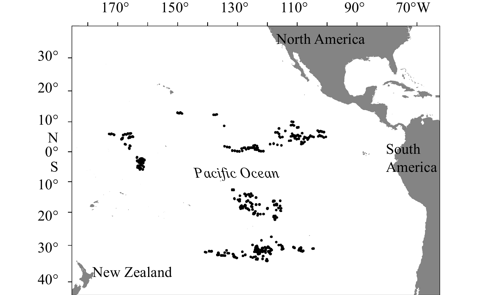
According to the simplified food web constructed in the central and eastern tropical Pacific food web (Lin and Zhu, 2020) in terms of topological importance analysis and species’ economic value, we selected twenty species (Table 1) and projected their population dynamics under different fishing levels. These twenty species accounted for over 90% of the total catch of all species collected by China’s tuna longline observers in the central and eastern tropical Pacific from June to November, 2017 (Fig. 1). Trip information was listed in Table S1, and more details are available in China’s annual report provided to the WCPFC Commission (Dai et al., 2017). In addition to the relatively higher abundances in the ecosystem, these species play critical roles in maintaining food web structure and stability and reflecting population dynamics in a multispecies size-structured community (Lin and Zhu, 2020). Nine large-sized species are our research priority, not only because of the data availability but also the primary interests of longline fishery in the tropical Pacific Ocean, including Yellowfin tuna (Thunnus albacares), Bigeye tuna (Thunnus obesus), Swordfish (Xiphias gladius), Blue marlin (Makaira mazara), Albacore tuna (Thunnus alalunga), Silky shark (Carcharhinus falciformis), Blue shark (Prionace glauca), Skipjack (Katsuwonus pelamis ) and Striped marlin (Kajikia audax). If measurable, the size, sex, and other biological information of fish were recorded by on-board observers. Also, the stomach samples were sent to the laboratory of Shanghai Ocean University for further analysis. Information on stomach content samples, including length (mm), weight (g), and quantity of prey items, were measured. The detailed feeding relationships among the nine species in the ecosystem have been introduced in Feng et al. (2019) and are not repeated here.
Table
1.
Species-specific input parameters used in the size-spectrum model
Figure
1.
Location of Chinese longline fishery in the central and eastern tropical Pacific from June to November in 2017. Each dot represents a position where a longline set was deployed.
In the multispecies size-spectrum model, each species shows different change patterns driven by specific life history characteristics, including growth, predation, mortality, and reproduction (Andersen and Beyer, 2006; Hartvig et al., 2011; Scott et al., 2014). A governing principle in the size-spectrum model is that the available energy gets from predation by larger species on smaller ones and used for growth and reproduction can be linked to the asymptotic size of the predator (Ursin, 1973; Andersen et al., 2015).
The model framework builds on two generally accepted ecological assumptions. The first is that an essential trait of a species, i, is its body weight, w, and the model can be formulated with several general parameters as all the other parameters are relevant to the body weight. The population dynamics of a given species that are driven by growth and mortality can be formulated by the McKendrick-von Foerster Conservation Equation (M’Kendrick, 1925; von Foerster, 1959):
where gi(w) is the individual growth at weight w, and μi(w) is the total mortality of species i, t is time. The size spectrum Ni(w) of a particular size class in the model can be measured in the unit of numbers per weight per volume (Andersen and Pedersen, 2010). The second assumption is that the food preference (ϕ) depends on the species and the individual weight, described by the log-normal selection model (Ursin, 1973):
where w and wp are the bodyweights of the predator and prey, respectively. βi is the preferred predator-prey mass ratio, and σi is the width of the size selection function. Details of other equations (Hartvig et al., 2011; Andersen et al., 2016b) are listed in Table 2. A set of default parameters is listed in Table S2, and the interaction matrix (θ) estimated based on species’ vertical overlap is included in Table S3 (Woodworth-Jefcoats et al., 2019).
Note: $\kappa $ in Eq. (4) is the abbreviation of carrying capacity; p in Eq. (7) and Eq. (8) represents the exponent of standard metabolism and the default value in the model is 0.75; $\epsilon $ in Eq. (11) is the efficiency of offspring production; SS in Eq. (14) is the selectivity size; r0 in Eq. (15) is the coefficient of regeneration rate of resources, and the default values in the model are 0.1 and 4, respectively; $\text{λ} $ in the Eq. (16) is the exponent of resource spectrum following the equation 2−n+q, where n is the exponent for maximum food intake (2/3) and q is the exponent for volumetric search rate (0.8). Other default parameters are listed in Table S2.
The encounter rate of food Ei(w) (Eq. (3)) among individuals is based on the “Andersen-Ursin” encounter model (Andersen and Ursin, 1977). Both small-sized species and zooplankton which is part of the background resource can be considered as available food. The combination of food preference, volumetric search rate Vi(w) (Eq. (4)), and prey abundance determine the food encounter rate. The consumption of an individual after predation is related to the feeding level, fi(w) (Eq. (5)), ranging from 0 to 1, and the maximum consumption rate Imax, i(w) (Eq. (6)).
The energy obtained by effective assimilation of ingested food is used to meet the needs of standard metabolism, partly for somatic growth gi(w) (Eq. (7)) of juveniles and partly for reproduction and maturation $\psi $i(w) (Eq. (8)) of mature individuals. Species’ growth and reproduction will stop if the food supply fails to support the metabolic requirements. And the allocation proportion between somatic growth and reproduction is determined by the maturation function $\psi $i(w) (Eq. (9)) of individuals. The recruitment Ri (Eq. (10)) described by a Beverton-Holt type function (Beverton and Holt, 1957) is dependent on the amount of energy used for reproduction Rep (Eq. (11), calculated as the number of eggs); and the maximum recruitment Rmax, i (numbers of surviving recruits every year) as a key parameter essentially decides the total biomass of a population. The mortality of an individual has three categories: predation mortality μp, i(w) (Eq. (12)), background mortality μb, i(w) (Eq. (13)), and fishing mortality, Fi(w) (Eq. (14)), which ensures a mass balance in the size-spectrum model. Fishing was imposed with the default knife-edge selectivity in the size-spectrum framework. The catchability (Qi) was set to a constant value of 1 in the simulation.
The resource spectrum Nr(w) (Eq. (15)) acts as the food items of the smallest individuals, which prey on zooplankton or benthic production. The resource dynamics can be modeled by a semi-chemostat growth equation combined with a carrying capacity $\kappa(w) $ (Eq. (16)) defined as the control parameter for the resource productivity in the community.
The size-spectrum model can be implemented by the R package “mizer” (Scott et al., 2014).
2.2
Model parameterization and validation
Each of the twenty species is characterized by a range of parameters reflecting its species-specific physiological features and life history (Table 1). K is the growth coefficient; a and b are the parameters in weight-length relationships. Winf and Wmat represent the asymptotic body weight and mature weight of species, respectively. Species’ maximum size obtained from FishBase was converted to Winf following the standard exponential equation W =aLb. The above five growth parameters were publicly available from FishBase. Following previous studies, β, the preferred predator-prey mass ratio was assigned 100 for species fed mostly on fish, 400 for shark species, and 1000 for species with strong dependencies on zooplanktons (Blanchard et al., 2014; Reum et al., 2019). The initial Rmax was estimated from an empirical equation as 1011×$W_{\rm{inf}}^{-1.5} $ (Blanchard et al., 2014). The Rmax and default carrying capacity of background resources ($\kappa $) were then calibrated by minimizing the Root Mean Square Error (RMSE) between the log-transformed modelled and estimated spawning stock biomass (SSB) from the WCPFC single stock assessments of the nine large-sized species from 1993 to 2012 (20 years’ fishing period). RMSE is a frequently used measure of the differences between values predicted by a model and the values observed. According to Chai and Draxler (2014), the calculation of RMSE was expressed as:
The time-series fishing mortality (1952−2015) used for model validation were also derived from the most recent WCPFC stock assessment reports. Many of these species are non-target species in the longline fishery that are lacking fishing mortality data. The fishing mortality of bycatch species has increased about fourfold, owing to increases in effort in tuna fisheries in the Pacific Ocean (Shelley et al., 2014). Thus, we assumed that fish mortality of these species increases linearly (from 0 to 0.4) at this time period. The selectivity size (SS) parameters of each species are different. The size position susceptible to fishing mortality of each species was determined by the asymptotic size following the equation as Winf×0.05 (Scott et al., 2013). Cephalopods, Scomber, and Puffer are not sorted to species level, and the parameter estimates were averaged from several representative species. Besides, parameters of some species were obtained from relevant studies when biological data were not available in FishBase. Detailed sources were noted in Table 1.
The constructed size-spectrum model was first to run for 200 a before 1952 without fishing mortality for all species to get the virgin resources before the fishing efforts were introduced. The initial population abundances play a decisive role in determining the population dynamics in a community. We also run the model under historical fishing mortality from 1952 to 2015 to reach the current state of the community. In addition, after the calibration of Rmax and $\kappa $, we compared the simulated growth curves with empirical size-at-age data to ensure that the calibrated model could produce plausible stock dynamics. R-squared (R2) ranging from 0 to 1 was used to indicate the statistical measure of fit between two sets of data. The changing trend between predictions and observations can better demonstrate the goodness of fit than a specific value matched in a given time period (Jacobsen et al., 2017). Most species in the size-spectrum model began to be exploited in the 1950s. Some species started being fished in the 1970s, and the fishing mortality was set to 0 in the 1950s to 1970s, including Blue shark, Silky shark, Blue marlin, and Skipjack.
2.3
Scenario projections and analysis of model outputs
We used the calibrated model to predict the dynamic changes of nine species in the community from 2016 to 2050 under five fishing scenarios:
(1) unexploited Scenario: F= 0;
(2) recent F Scenario: F=Frecent, the average fishing mortality from 2013 to 2015;
(3) low F Scenario: F=0.5Frecent;
(4) medium F Scenario: F=2Frecent;
(5) high F Scenario: F=3Frecent.
The recent fishing mortality (Frecent) for nine species obtained from WCPFC stock assessment outputs was listed in the Table S4. These scenarios were chosen partly based on the fishing history of each species in the Pacific Ocean and can help us understand the fishery status of the target species relative to the unfished ecosystem. The total biomass, mean body weight (MeanW), and the slope of community size spectra (Slope) were used as ecological indicators to reflect the changes in species abundance and ecosystem structure.
3.
Results
3.1
Model Validation
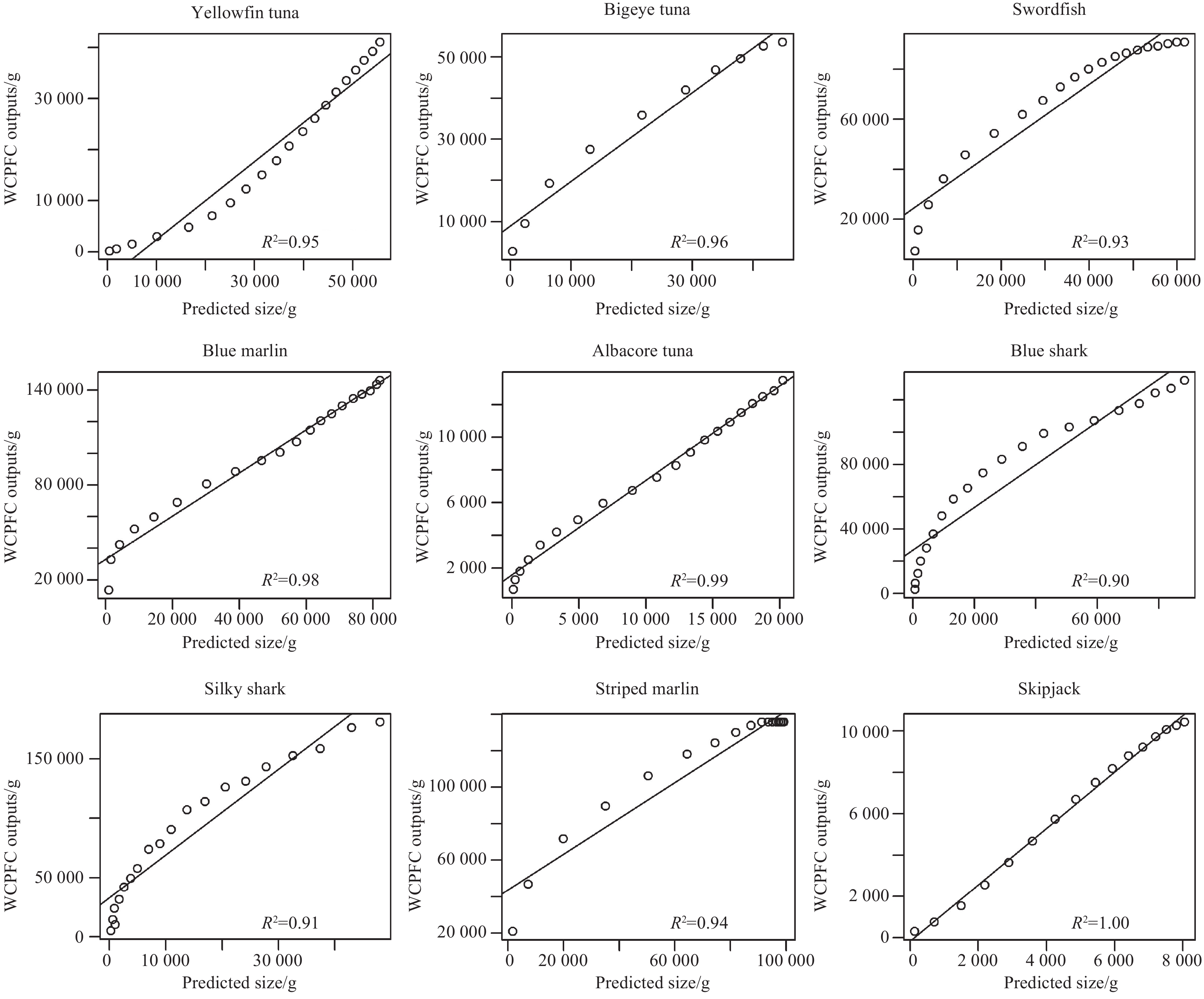
Following previous studies, we calibrated the model by tuning two influential parameters Rmax and kappa, which are essential for setting species’ initial size spectra and determines the background resource in the system. The validation results were demonstrated in Fig. 2. The model produced strong correlations between the size-at-age data from our simulation and the WCPFC reports, with the R2 of nine species more than 0.9. Therefore, the model validation results indicated that the multispecies size-spectrum model could reflect the dynamics of a fish community in the tropical Pacific.
Figure
2.
Model validation results. Comparison of species’ size-at-age data modeled in this study with the outputs in the WCPFC stock assessment reports. The closer R2 is to 1, the better the fit is.
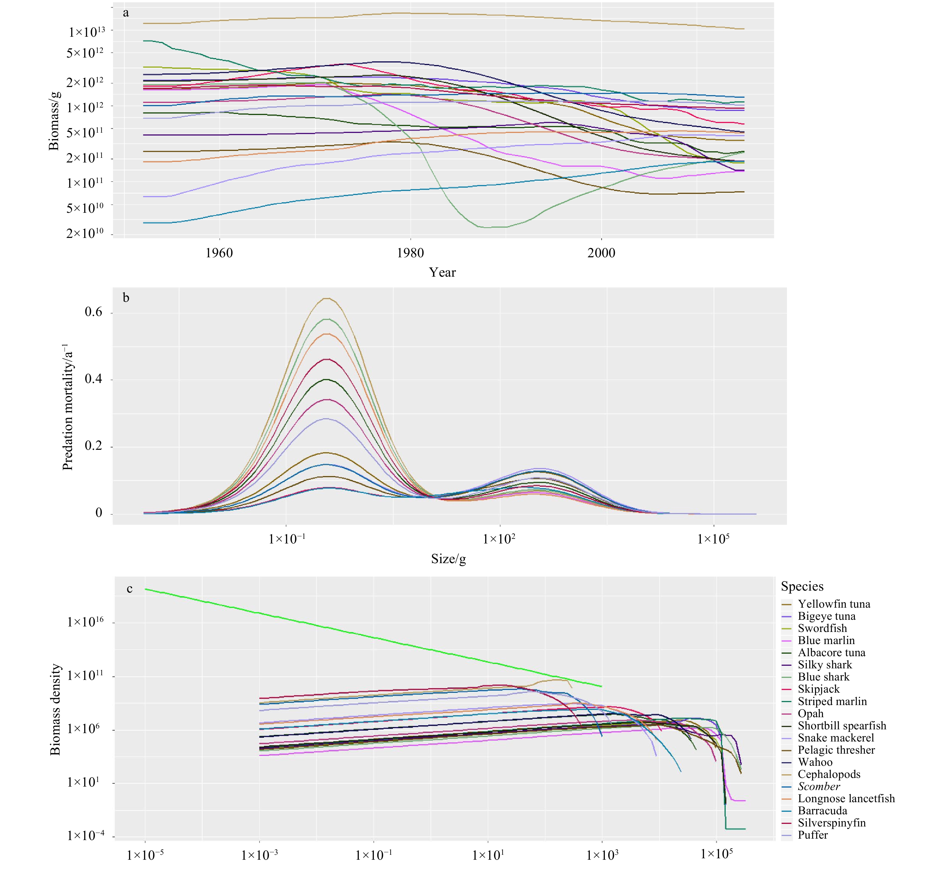
The multispecies size-spectrum model projects the dynamics of individual species. As shown in Fig. 3, all species showed different patterns driven by specific parameters, including biomass (Fig. 3a), predation mortality (Fig. 3b), and biomass spectra (Fig. 3c). It can be seen that predation mortality increased firstly and then varies with the increasing body size. There are two “bumps” of the predation mortality curve due to the trophic cascade effect. The enormous individuals in the community do not experience predation by other species. Species biomass fluctuated continuously. The economic species showed a slight downward trend under the historical fishing mortality, except that the biomass of Blue shark began to increase since 1990. The biomass of several species tended to reach a balance over time, such as Bigeye tuna and Blue marlin. The biomass density of large-sized species declined dramatically following historical fishing (Fig. 3c).
Figure
3.
The outputs of the multispecies size-spectrum model when historical fishing efforts from 1952 to 2015 were applied. Each line presents one of the species in the community. The biomass (a) change through time was demonstrated, and predation mortality (b) and biomass density (c) were the reflection of the last fishing year (2015).
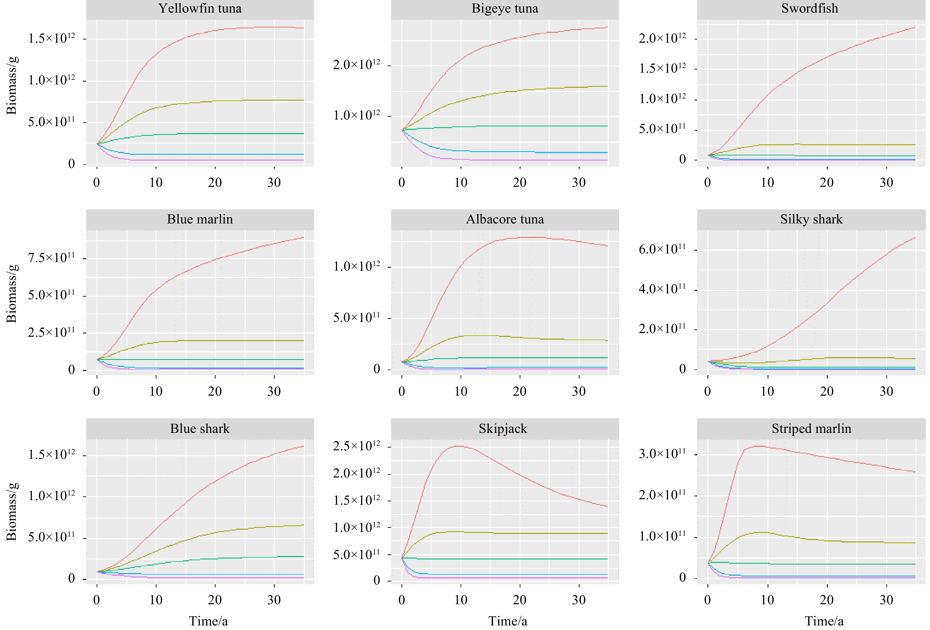
Figure 4 demonstrated the projected biomass change of nine large-sized species caught by longline fishery from 2016 to 2050. The simulation results indicated that each species responded differently to fishing activities, and the decline in biomass was not proportional to the increase in fishing mortality. The biomass of nine species showed an upward trend over the projection period without fishing. The biomass of the main target tuna species in the community was still abundant by 2050 under the recent fishing level, except Albacore tuna. When the fishing mortality was increased to two or three times of Frecent, the biomass of these species decreased dramatically in a few years. We also found that the biomass of Silky shark remained at relatively low levels by 2050 when the fishing mortality was halved (0.5Frecent).
Figure
4.
Projected biomass of nine large-sized species under different fishing scenarios: F=0 (red), F=Frecent (yellow), F=0.5Frecent (green), F=2Frecent (blue), F=3Frecent (purple).
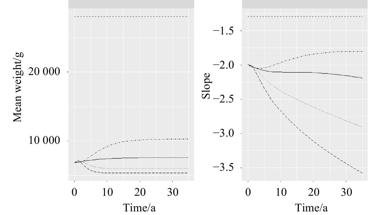
Figure 5 presents the changes of ecological indicators under five fishing scenarios from 2016 to 2050. The dashed lines (F=0) denote an unexploited community, where the MeanW and Slope are both stable. The direct effect of fishing on the community structure was the decrease of the abundance of large-sized individuals, which could be reflected in the declining MeanW and steepening of the size spectrum. Under the 2Frecent Scenario, species’ mean weight decreased about 1 500 g (21%) by 2050 compared with that under the Frecent Scenario. The community Slope indicated a more obvious downward trend with the increasing fishing mortality.
Figure
5.
Ecological indicators respond to different fishing levels over the projection time period (2016−2050), including mean body weight (MeanW in g) and slope of community size spectra (Slope). Dashed line, solid line, dot-dash line, dotted line, and longdash line represent fishing scenarios of F=0, F=Frecent, F=0.5Frecent, F=2Frecent, and F=3Frecent, respectively.
We developed a multispecies size-spectrum framework to analyze and predict the dynamics of species in the central and eastern tropical Pacific ecosystem. The methods provide a convenient way to explore the responses of the community to different fishing levels (Scott et al., 2013). The size-spectrum model has the advantage of maintaining ecological realism compared with traditional unstructured models (Andersen et al., 2016a; Zhang et al., 2018). Most parameters in the model can be obtained from a cross-species analysis (Hartvig et al., 2011) and the metabolic theory (Brown et al., 2004). The model is based on individual-level ecological processes. In Fig. 3, the biomass and mortality of each species responded differently to historical fishing mortality; the situation was mainly determined by size structure. The simulation results also confirmed the importance of species’ specific life history and their interactions with other species in sustaining ecosystem structure. Many species in our study are non-tuna bycatch species retained as byproducts in the commercial longline fishery. However, stock assessments have only been undertaken on very few stocks of non-tuna species, and the absence of information impacting the ability to make informed management decisions.
The tropical Pacific Ocean is large enough to ignore the migration effects for most species. Meanwhile, there are sufficient spatial overlaps among species to ensure regular species interactions, as shown in Table S3. Many previous studies on the Pacific Ocean were primarily based on data from adjacent areas due to the difficulties of obtaining samples in open-ocean (Worm et al., 2005; Gerrodette et al., 2012; Zhu et al., 2012). Thus, the acquisition of the Chinese tuna longline observer data can prompt the reliability of our study. However, our results may only reflect part of pelagic ecosystem dynamics because most of our species are top predators caught by pelagic longlines. In addition, we validated the SSBs and size-at-age data of nine species, but that may not guarantee a reliable projection of the whole ecosystem (Andersen et al., 2016b).
Another limitation of this study is that we only considered the effects of fishing on community structure. Climate-driven pressures such as changes in water temperature and ocean circulation may also threaten the survival of species, impact species distributions and change the community structure (Genner et al., 2010; Simpson et al., 2011). Secondly, we used the MeanW, Slope, and total biomass to reflect the responses of the community to different fishing levels. The study of Houle et al. (2012) revealed that length-based indicators weighted by biomass were more sensitive to fishing pressure. However, these indicators we analyzed may not reflect the population dynamics and ecosystem structure in all respects. The dynamic changes of ecosystem structure leading by fishing are nonlinear in the size-spectrum model. The response of community indicators is usually more sensitive at a smaller fishing effort level (Houle et al., 2012; Zhang et al., 2016). Therefore, as shown in Fig. 4, the species’ biomass showed a disproportionate changing pattern partly due to the different sensitivities to fishing mortality and indirect trophic effects in the community. This size-spectrum model would generate more complex results since a change in fishing effort generally does not result in a proportional change in relevant community indicators. Thus, more attempts to explore the sensitivity of different indicators in fishing are encouraged (Rochet and Trenkel, 2003; Houle et al., 2012).
The simulation results (Fig. 5) in this study are consistent with the conjecture that continuing fishing activities leads to a steepening of the spectrum (Rice and Gislason, 1996; Shin and Cury, 2004; Shin et al., 2005). A reason for this consistency is that fishing mainly targets large-sized individuals. Populations with small asymptotic sizes have larger abundances than those with large asymptotic sizes throughout the life history (Scott et al., 2014). We did not specify the species’ catchability. The default value is set to 1 in the simulation, which means that the fully-selected individuals of a species would be caught efficiently under fishing. Fishing reduces the abundance of small fishes, but compared with natural predation mortality, the fishing effects are relatively low (Andersen and Pedersen, 2010). Also, the reduction of prey resources affects the food availability of their predators; thus, large individuals would have a slower growth rate. In other words, the same fishing effort level had a limited impact on smaller-sized species compared to large-sized predators in our study. Combined with the projection results in Fig. 4, species will not become extinct under long-term fishing only by adopting the most practical management measures. That is to say, there must be sufficient large-sized individuals within a population. Therefore, the recent fishing efforts of Blue marlin and Silky shark need to be adjusted according to the evaluation results and actual situation. The study of Schindler and Hilborn (2015) also revealed that the size-spectrum model is more suitable for short-term predictions, which can be considered as a reference when deciding management strategies.
The fishing impacts triggered by the removal of top predators can also be described as a trophic cascade (Andersen and Pedersen, 2010). A trophic cascade is a sign of indirect impacts among species and can occur in various marine ecosystems when the species abundance at different sizes change due to fishing (Myers et al., 2007; Casini et al., 2008). The phenomenon can be explored by comparing the relative abundance changes of all individuals at different size ranges of F=Frecent, F=3Frecent, and unexploited community (Fig. 6). Compared with the recent fishing scenario, the abundance of large-sized species decreased sharply under the high fishing scenario, consistent with the results shown in Fig. 5. The constant F=0 prediction was used as the baseline, which is also a fundamental assumption proposed by Sheldon et al. (1972) about species size distribution in the marine ecosystem. The effects of fishing on relative abundance vary with the increasing individual size. The fishing pressure reduces the abundance of large-sized individuals. The abundance of smaller individuals will increase due to the release from predation by their predators, which is accordant with the results in the North Sea fish community (Daan et al., 2005). Similarly, this increases the predation mortality on their prey, thus reducing the abundances of the prey species. Subsequently, the fishery will begin to target medium-sized individuals, which will lead to changes in ecosystem structure.
Figure
6.
The relative abundance of different size individuals in the size-spectrum model when F=0 (dashed line), F=Frecent (solid line), and F=3Frecent (red line).
This study modelled a realistic fish community in the central and eastern tropical Pacific Ocean under different fishing scenarios. The response of nine ecologically and economically important species suggested that only the biomass of Bigeye tuna, Swordfish, Yellowfin tuna, and Skipjack could maintain a stable abundance under the recent fishing mortality. Current management strategies are insufficient to achieve an optimal balance between conservation objectives and exploitation of fishery resources, especially for sharks and billfishes. Ecosystem-based fisheries management is an effective way to minimize potential impacts on the ecosystem while realizing sustainable utilization of fishery resources. In an ecosystem context, it is needed to explore the community dynamics under simultaneous stressors such as fishing and environmental changes and consider various complementary indicators in the simulation analysis. In addition, biological research and rigorous stock assessments of non-tuna species captured in the longline fishery should be a high research priority. Thus, relevant studies can better inform and advise fisheries management.
Andersen K H, Beyer J E. 2006. Asymptotic size determines species abundance in the marine size spectrum. The American Naturalist, 168(1): 54–61. doi: 10.1086/504849
[2]
Andersen K H, Blanchard J L, Fulton E A, et al. 2016a. Assumptions behind size-based ecosystem models are realistic. ICES Journal of Marine Science, 73(6): 1651–1655
[3]
Andersen K H, Brander K, Ravn-Jonsen L. 2015. Trade-offs between objectives for ecosystem management of fisheries. Ecological Applications, 25(5): 1390–1396. doi: 10.1890/14-1209.1
[4]
Andersen K H, Jacobsen N S, Farnsworth K D. 2016b. The theoretical foundations for size spectrum models of fish communities. Canadian Journal of Fisheries and Aquatic Sciences, 73(4): 575–588. doi: 10.1139/cjfas-2015-0230
[5]
Andersen K H, Pedersen M. 2010. Damped trophic cascades driven by fishing in model marine ecosystems. Proceedings of the Royal Society B: Biological Sciences, 277(1682): 795–802. doi: 10.1098/rspb.2009.1512
[6]
Andersen K P, Ursin E. 1977. A multispecies extension to the Beverton and Holt theory of fishing: with accounts of phosphorus circulation and primary production. Meddelelser fra Danmarks Fiskeri- og Havundersø gelser, 7: 319–435
[7]
Bauer B, Horbowy J, Rahikainen M, et al. 2019. Model uncertainty and simulated multispecies fisheries management advice in the Baltic Sea. PLoS ONE, 14(1): e0211320. doi: 10.1371/journal.pone.0211320
[8]
Beverton R J H, Holt S J. 1957. On the Dynamics of Exploited Fish Populations. Fisheries Investigations Series 2, Volume 19. London: U. K. Ministry of Agriculture and Fisheries, 1–533
[9]
Billfish Working Group Report. 2015. Stock assessment update for striped marlin (Kajikia audax) in the Western and Central North Pacific Ocean through 2013. Kona, HI, USA: International Scientific Committee for Tuna and Tuna-like Species in the North Pacific Ocean, 97
[10]
Billfish Working Group Report. 2016. Stock assessment update for blue marlin (Makaira nigricans) in the Pacific Ocean through 2014. Sapporo, Hokkaido, Japan: International Scientific Committee for Tuna and Tuna-like Species in the North Pacific Ocean, 90
[11]
Blanchard J L, Andersen K H, Scott F, et al. 2014. Evaluating targets and trade-offs among fisheries and conservation objectives using a multispecies size spectrum model. Journal of Applied Ecology, 51(3): 612–622. doi: 10.1111/1365-2664.12238
[12]
Brown J H, Gillooly J F, Allen A P, et al. 2004. Toward a metabolic theory of ecology. Ecology, 85(7): 1771–1789. doi: 10.1890/03-9000
[13]
Casini M, Lövgren J, Hjelm J, et al. 2008. Multi-level trophic cascades in a heavily exploited open marine ecosystem. Proceedings of the Royal Society B: Biological Sciences, 275(1644): 1793–1801. doi: 10.1098/rspb.2007.1752
[14]
Chai T, Draxler R R. 2014. Root mean square error (RMSE) or mean absolute error (MAE)? —Arguments against avoiding RMSE in the literature. Geoscientific Model Development, 7(3): 1247–1250. doi: 10.5194/gmd-7-1247-2014
[15]
Collie J S, Botsford L W, Hastings A, et al. 2016. Ecosystem models for fisheries management: finding the sweet spot. Fish and Fisheries, 17(1): 101–125. doi: 10.1111/faf.12093
[16]
Daan N, Gislason H, Pope J G, et al. 2005. Changes in the North Sea fish community: evidence of indirect effects of fishing?. ICES Journal of Marine Science, 62(2): 177–188. doi: 10.1016/j.icesjms.2004.08.020
[17]
Dai Xiaojie, Wu Feng, Wang Xuefang. 2017. Annual report to the commission Part 1: information on fisheries, research and statistics. Information paper SC13-AR/CCM-03. In: Report to Thirteenth Regulation Session of the WCPFC Scientific Committee (SC13). Rarotonga, Cook Islands: Western and Central Pacific Fisheries Commission
[18]
DeMartini E E, Uchiyama J H, Williams H A. 2000. Sexual maturity, sex ratio, and size composition of swordfish, Xiphias gladius, caught by the Hawaii-based pelagic longline fishery. Fishery Bulletin, 98(3): 489–506
[19]
Dulvy N K, Polunin N V C, Mill A C, et al. 2004. Size structural change in lightly exploited coral reef fish communities: evidence for weak indirect effects. Canadian Journal of Fisheries and Aquatic Sciences, 61(3): 466–475. doi: 10.1139/f03-169
[20]
Farley J, Eveson P, Krusic-Golub K, et al. 2017. Project 35: Age, growth and maturity of bigeye tuna in the western and central Pacific Ocean. Working paper WCPFC-SC13-2017/SA-WP-01 Rev 1. In: Report to Thirteenth Regulation Session of the WCPFC Scientific Committee (SC13). Rarotonga, Cook Islands: Western and Central PacificFisheries Commission
[21]
Feng Huili, Zhu Jiangfeng, Chen Yan. 2019. Construction and historical comparison of ecosystem structure of the eastern tropical Pacific Ocean based on Ecopath model. Journal of Shanghai Ocean University, 28(6): 921–932
[22]
Food and Agricultural Organization of the United Nations. 2001. What is the code of conduct for responsible fisheries?. Rome, Italy: Food and Agricultural Organization of the United Nations
[23]
Francis M, Griggs L, Maolagáin C Ó. 2004. Growth rate, age at maturity, longevity and natural mortality rate of moonfish (Lampris guttatus). In: Final Research Report for the Ministry of Fisheries Research Project TUN2003-01. Taihoro, Nukurangi: National Institute of Water and Atmospheric Research
[24]
Genner M J, Sims D W, Southward A J, et al. 2010. Body size-dependent responses of a marine fish assemblage to climate change and fishing over a century-long scale. Global Change Biology, 16(2): 517–527. doi: 10.1111/j.1365-2486.2009.02027.x
[25]
Gerrodette T, Olson R, Reilly S, et al. 2012. Ecological metrics of biomass removed by three methods of purse-seine fishing for tunas in the eastern tropical Pacific Ocean. Conservation Biology, 26(2): 248–256. doi: 10.1111/j.1523-1739.2011.01817.x
[26]
Giacomini H C, Shuter B J, Baum J K. 2016. Size-based approaches to aquatic ecosystems and fisheries science: a symposium in honour of Rob Peters. Canadian Journal of Fisheries and Aquatic Sciences, 73(4): 471–476. doi: 10.1139/cjfas-2016-0100
[27]
Gibbs R H Jr. 1960. Alepisaurus brevirostris, a new species of lancetfish from the western North Atlantic. Museum of Comparative Zoology, 123: 1–14
[28]
Gislason H, Rice J C. 1998. Modelling the response of size and diversity spectra of fish assemblages to changes in exploitation. ICES Journal of Marine Science, 55(3): 362–370. doi: 10.1006/jmsc.1997.0323
[29]
Hartvig M, Andersen K H, Beyer J E. 2011. Food web framework for size-structured populations. Journal of Theoretical Biology, 272(1): 113–122. doi: 10.1016/j.jtbi.2010.12.006
[30]
Houle J E, Farnsworth K D, Rossberg A G, et al. 2012. Assessing the sensitivity and specificity of fish community indicators to management action. Canadian Journal of Fisheries and Aquatic Sciences, 69(6): 1065–1079. doi: 10.1139/f2012-044
[31]
Jacobsen N S, Burgess M G, Andersen K H. 2017. Efficiency of fisheries is increasing at the ecosystem level. Fish and Fisheries, 18(2): 199–211. doi: 10.1111/faf.12171
[32]
Jacobsen N S, Essington T E, Andersen K H. 2015. Comparing model predictions for ecosystem-based management. Canadian Journal of Fisheries and Aquatic Sciences, 73(4): 666–676
[33]
Jacobsen N S, Gislason H, Andersen K H. 2014. The consequences of balanced harvesting of fish communities. Proceedings of the Royal Society B: Biological Sciences, 281(1775): 20132701. doi: 10.1098/rspb.2013.2701
[34]
Jennings S, Greenstreet S P R, Reynolds J D. 1999. Structural change in an exploited fish community: a consequence of differential fishing effects on species with contrasting life histories. Journal of Animal Ecology, 68(3): 617–627. doi: 10.1046/j.1365-2656.1999.00312.x
[35]
Law R. 2000. Fishing, selection, and phenotypic evolution. ICES Journal of Marine Science, 57(3): 659–668. doi: 10.1006/jmsc.2000.0731
[36]
Lin Qinqin, Zhu Jiangfeng. 2020. Topology-based analysis of pelagic food web structure in the central and eastern tropical Pacific Ocean based on longline observer data. Acta Oceanologica Sinica, 39(6): 1–9. doi: 10.1007/s13131-020-1592-2
[37]
M’Kendrick A G. 1925. Applications of mathematics to medical problems. Proceedings of the Edinburgh Mathematical Society, 44: 98–130. doi: 10.1017/S0013091500034428
[38]
Miyake M, Guillotreau P, Sun C H, et al. 2010. Recent developments in the tuna industry: stocks, fisheries, management, processing, trade and markets. FAO Fisheries and Aquaculture Technical Paper, 543: 1–125
[39]
Myers R A, Baum J K, Shepherd T D, et al. 2007. Cascading effects of the loss of apex predatory sharks from a coastal ocean. Science, 315(5820): 1846–1850. doi: 10.1126/science.1138657
[40]
Pauly D, Christensen V, Dalsgaard J, et al. 1998. Fishing down marine food webs. Science, 279(5352): 860–863. doi: 10.1126/science.279.5352.860
[41]
Polovina J J, Abecassis M, Howell E A, et al. 2009. Increases in the relative abundance of mid-trophic level fishes concurrent with declines in apex predators in the subtropical North Pacific, 1996−2006. Fishery Bulletin, 107(4): 523–531
[42]
Polovina J J, Woodworth-Jefcoats P A. 2013. Fishery-induced changes in the subtropical Pacific pelagic ecosystem size structure: observations and theory. PLoS ONE, 8(4): e62341. doi: 10.1371/journal.pone.0062341
[43]
Reum J C P, Blanchard J L, Holsman K K, et al. 2019. Species-specific ontogenetic diet shifts attenuate trophic cascades and lengthen food chains in exploited ecosystems. Oikos, 128(7): 1051–1064. doi: 10.1111/oik.05630
[44]
Rice J, Gislason H. 1996. Patterns of change in the size spectra of numbers and diversity of the North Sea fish assemblage, as reflected in surveys and models. ICES Journal of Marine Science, 53(6): 1214–1225. doi: 10.1006/jmsc.1996.0146
[45]
Rochet M J, Trenkel V M. 2003. Which community indicators can measure the impact of fishing? A review and proposals. Canadian Journal of Fisheries and Aquatic Sciences, 60(1): 86–99. doi: 10.1139/f02-164
[46]
Schindler D E, Hilborn R. 2015. Prediction, precaution, and policy under global change. Science, 347(6225): 953–954. doi: 10.1126/science.1261824
[47]
Scott F, Blanchard J L, Andersen K H. 2013. Multispecies, Trait and Community Size Spectrum Ecological Modelling in R (Mizer). Luxembourg: Publications Office of the European Union, 196
[48]
Scott F, Blanchard J L, Andersen K H. 2014. mizer: an R package for multispecies, trait-based and community size spectrum ecological modelling. Methods in Ecology and Evolution, 5(10): 1121–1125. doi: 10.1111/2041-210X.12256
[49]
Sheldon R W, Prakash A, Sutcliffe W H Jr. 1972. The size distribution of particles in the ocean. Limnology and Oceanography, 17(3): 327–340. doi: 10.4319/lo.1972.17.3.0327
[50]
Shelley C, Sato M, Small C, et al. 2014. Bycatch in longline fisheries for tuna and tuna-like species: a global review of status and mitigation measures. FAO Fisheries and Aquaculture Technical Paper, 588: 1–199
[51]
Shin Y J, Cury P. 2004. Using an individual-based model of fish assemblages to study the response of size spectra to changes in fishing. Canadian Journal of Fisheries and Aquatic Sciences, 61(3): 414–431. doi: 10.1139/f03-154
[52]
Shin Y J, Rochet M J, Jennings S, et al. 2005. Using size-based indicators to evaluate the ecosystem effects of fishing. ICES Journal of Marine Science, 62(3): 384–396. doi: 10.1016/j.icesjms.2005.01.004
[53]
Sibert J, Hampton J, Kleiber P, et al. 2006. Biomass, size, and trophic status of top predators in the Pacific Ocean. Science, 314(5806): 1773–1776. doi: 10.1126/science.1135347
[54]
Simpson S D, Jennings S, Johnson M P, et al. 2011. Continental shelf-wide response of a fish assemblage to rapid warming of the sea. Current Biology, 21(18): 1565–1570. doi: 10.1016/j.cub.2011.08.016
[55]
Sissenwine M, Murawski S. 2004. Moving beyond “intelligent thinking”: advancing an ecosystem approach to fisheries. In: Perspectives on Ecosystem-based Approaches to the Management of Marine Resources. Marine Ecology Progress Series, 274: 269–303. doi: 10.3354/meps274269
[56]
Ursin E. 1973. On the prey size preferences of cod and dab. Meddelelser fra Danmarks Fiskeri-og Havundersø gelser, 7: 85–98
[57]
von Foerster H. 1959. Some remarks on changing populations. In: Stohlman J F, ed. The Kinetics of Cellular Proliferation. New York: Grune and Stratton, 382–407
[58]
Woodworth-Jefcoats P A, Blanchard J L, Drazen J C. 2019. Relative impacts of simultaneous stressors on a pelagic marine ecosystem. Frontiers in Marine Science, 6: 383. doi: 10.3389/fmars.2019.00383
[59]
Worm B, Sandow M, Oschlies A, et al. 2005. Global patterns of predator diversity in the open oceans. Science, 309(5739): 1365–1369. doi: 10.1126/science.1113399
[60]
Zhang Chongliang, Chen Yong, Thompson K, et al. 2016. Implementing a multispecies size-spectrum model in a data-poor ecosystem. Acta Oceanologica Sinica, 35(4): 63–73. doi: 10.1007/s13131-016-0822-0
[61]
Zhang Chongliang, Chen Yong, Xu Binduo, et al. 2018. Evaluating fishing effects on the stability of fish communities using a size-spectrum model. Fisheries Research, 197: 123–130. doi: 10.1016/j.fishres.2017.09.004
[62]
Zhu Jiangfeng, Xu Liuxiong, Dai Xiaojie, et al. 2012. Comparative analysis of depth distribution for seventeen large pelagic fish species captured in a longline fishery in the central-eastern Pacific Ocean. Scientia Marina, 76(1): 149–157. doi: 10.3989/scimar.03379.16C
Pablo Couve, Nixon Bahamon, Cristian M. Canales, et al. Systematic Review of Multi-Species Models in Fisheries: Key Features and Current Trends. Fishes, 2024, 9(10): 372. doi:10.3390/fishes9100372
Qinqin Lin, Yuying Zhang, Jiangfeng Zhu. Simulating the impacts of fishing on central and eastern tropical Pacific ecosystem using multispecies size-spectrum model[J]. Acta Oceanologica Sinica, 2022, 41(3): 34-43. doi: 10.1007/s13131-021-1902-3
Qinqin Lin, Yuying Zhang, Jiangfeng Zhu. Simulating the impacts of fishing on central and eastern tropical Pacific ecosystem using multispecies size-spectrum model[J]. Acta Oceanologica Sinica, 2022, 41(3): 34-43. doi: 10.1007/s13131-021-1902-3
Note: $\kappa $ in Eq. (4) is the abbreviation of carrying capacity; p in Eq. (7) and Eq. (8) represents the exponent of standard metabolism and the default value in the model is 0.75; $\epsilon $ in Eq. (11) is the efficiency of offspring production; SS in Eq. (14) is the selectivity size; r0 in Eq. (15) is the coefficient of regeneration rate of resources, and the default values in the model are 0.1 and 4, respectively; $\text{λ} $ in the Eq. (16) is the exponent of resource spectrum following the equation 2−n+q, where n is the exponent for maximum food intake (2/3) and q is the exponent for volumetric search rate (0.8). Other default parameters are listed in Table S2.
Figure 1. Location of Chinese longline fishery in the central and eastern tropical Pacific from June to November in 2017. Each dot represents a position where a longline set was deployed.
Figure 2. Model validation results. Comparison of species’ size-at-age data modeled in this study with the outputs in the WCPFC stock assessment reports. The closer R2 is to 1, the better the fit is.
Figure 3. The outputs of the multispecies size-spectrum model when historical fishing efforts from 1952 to 2015 were applied. Each line presents one of the species in the community. The biomass (a) change through time was demonstrated, and predation mortality (b) and biomass density (c) were the reflection of the last fishing year (2015).
Figure 4. Projected biomass of nine large-sized species under different fishing scenarios: F=0 (red), F=Frecent (yellow), F=0.5Frecent (green), F=2Frecent (blue), F=3Frecent (purple).
Figure 5. Ecological indicators respond to different fishing levels over the projection time period (2016−2050), including mean body weight (MeanW in g) and slope of community size spectra (Slope). Dashed line, solid line, dot-dash line, dotted line, and longdash line represent fishing scenarios of F=0, F=Frecent, F=0.5Frecent, F=2Frecent, and F=3Frecent, respectively.
Figure 6. The relative abundance of different size individuals in the size-spectrum model when F=0 (dashed line), F=Frecent (solid line), and F=3Frecent (red line).


 DownLoad:

 DownLoad:


 DownLoad: