Temporal and spatial distribution characteristics of nutrients in Clarion-Clipperton Fracture Zone in the Pacific in 2017

1. Introduction

Deep-sea polymetallic nodules are potential sources of metals such as Fe, Mn, Ni, Cu and Co. Although deep-sea polymetallic nodules have been found in all oceans, only some areas have abundant nodule resources rich in elements of economic interest, and Clarion-Clipperton Fracture Zone (CCFZ) in the eastern tropical Pacific is one of these important areas causing growing interest in mining them (Wu et al., 2013). For this reason, 16 exploration contracts for large nodule fields within the CCFZ have been granted by the International Seabed Authority (ISA). Recent studies have demonstrated that planned mining activities have serious negative environmental impacts, and the post-disturbance recovery of the impacted ecosystem will be an extremely long process, measured in the scale of decades or even thousands of years (Jones et al., 2017). Because of concerns about the effects of mining on the functioning of deep-sea ecosystems and biodiversity, the ISA has identified “Areas of Particular Environmental Interest”. In the past few decades, as an important region for its role in climate variability due to the El Niño-Southern Oscillation (ENSO), in fish production, and in the global carbon cycle (Fiedler and Lavin, 2006), under the framework of the Tropical Ocean and Global Atmosphere and the World Ocean Circulation Experiment, there have been a number of observational investigation programs in the eastern tropical Pacific. However, studies about biogeochemical processes of nutrients in this area is still relatively insufficient to resolve seasonal and ENSO variability (Fiedler and Talley, 2006). As one part of the eastern tropical Pacific, reports about the baseline or changes of the environmental conditions in CCFZ are still insufficient (Menendez et al., 2019; Tu, 2006). As the primary elements of marine life, the distribution or circulation of nutrients in the ocean is important to understand the primary production or changes of marine ecosystem. However, studies about spatial and temporal changes of nutrients in CCFZ are still scares (Loubere, 2001; Tu, 2006). Therefore, here we present a study on (1) the baseline of spatial distribution characteristics of nutrients in 2017 and their physical or biological controlling factors, and (2) temporal changes of nutrient concentrations and molar ratios, comparing with the baseline investigation in 1990s−2000s. The main scientific objectives of this study are to give data basis to (1) discuss long-term changes of nutrient concentrations in CCFZ, (2) evaluate ecological changes in CCFZ under the background of eastern tropical Pacific, and (3) help to develope polymetallic nodules in CCFZ .

2. Methods

2.1 Study area

CCFZ is located in the eastern tropical Pacific, north of the equatorial zone. It comprises an area of about 6×10⁶ km², defined by two major transform faults, the Clarion Fracture Zone in the north and the Clipperton Fracture Zone in the south (Volz et al., 2018), extending from approximately 20°N, 120°W to 5°N, 160°W, with a total length of 7240 km (Menendez et al., 2019). Eastern tropical Pacific containing both the eastern terminus of the equatorial current system of the Pacific (Kessler, 2006) and the eastern Pacific warm pool that forms half of the western hemisphere warm pool straddling Central America (Wang and Enfield, 2001). The current in the north of eastern tropical Pacific is one of the most important current systems in the whole ocean circulation. This study area is mainly under the control of North Equatorial Current, South Equatorial Current and North Equatorial Countercurrent. In the west of this area is the warm tongue extending from the east of the western Pacific warm pool, and in the south of the area is the equatorial cold water tongue. The upper ocean in this area is mainly affected by these currents and water masses, and the flowing direction and velocity of the surface current are affected by ENSO events (Tu, 2006). Under the control of the northeast trade wind all the year round, the study area has the characteristics of paroxysmal and frequent precipitation because of its low latitude. And the study area belongs to the East Pacific Basin. From east to west, the water depth gradually deepens. While from north to south, the water depth gradually becomes shallow and the change range is small (Tu, 2006). Considering that abyssal benthic communities are limited by low carbon export from the euphotic zone (Smith et al., 2008), biodiversity in the CCFZ is surprisingly high (Glover et al., 2002). And as a consequence of microbial respiration in the water column and weak ocean ventilation, a pronounced oxygen minimum zone persists in the eastern equatorial Pacific (Kalvelage et al., 2015).

2.2 Sampling collection

Eight stations were investigated in Chinese contract area in CCFZ in this cruise (Fig. 1 and Table 1), from August 21 to October 8 in 2017, which was organized by Third Institute of Oceanography, Ministry of Natural Resources of China. At each station, temperature (T), salinity (S), pressure and chlorophyll a (Chl a) concentration were recorded by a conductivity-temperature-depth (CTD) profiler (Sea-Bird, SBE 911plus, Table 2). Water samples were collected at different layers (5 m, 50 m, 75 m, 100 m, 200 m, 500 m, 1000 m, 2500 m, 4500 m, 5000 m) with Niskin bottles mounted onto a rosette sampler attached to the CTD. Nutrients (${\rm{NO}}_3^ -{\text -} {\rm{N}} $, ${\rm{NO}}_2^ -{\text -} {\rm{N}} $, ${\rm{NH}}_4^+ {\text - }{\rm {N}} $, ${\rm{PO}}_4^{3 - }{\text -}{\rm{P}} $ and ${\rm{SiO}}_3^{2 - } {\text -} {\rm{Si}}$) and dissdved oxygen (DO) were sampled according to the Specification of Oceanographic Survey—Part 4: Survey of Chemical Parameters in Sea Water (General Administration of Quality Supervision, Inspection and Quarantine of the People’s Republic of China and Standardization Administration, 2008; Chen et al., 2014). About 500 mL water samples were filtered immediately through pre-cleaned 0.45 μm pore filters to collect nutrients samples. Then nutrients samples were preserved at a low temperature (4°C) in an ice box and analyzed on board in 24 h (General Administration of Quality Supervision, Inspection and Quarantine of the People’s Republic of China and Standardization Administration, 2008).

Figure  1.  Map of the investigation area in CCFZ. The triangle represents the location of stations in seamounts of the subtropical western Pacific Ocean, the circle represents Station ALOHA.

DownLoad: Full-Size Img PowerPoint

Table  1.  Location and water depth of sampling stations in 2017

Station	Latitude	Longitude	Date	Depth/m
CC-S06	12°58.115 1' N	153°14.585 2' W	Agu. 21	5 447
CC-S01	8°30.025 6' N	154°15.151 1' W	Agu. 25	5 187
KW1-S37	9°30.103 0' N	154°14.884 1' W	Spet. 4−5	5 133
KW1-S05	10°04.973 9' N	154°20.038 5' W	Sept. 9−10	5 173
KW1-S01	11°00.011 8' N	154°15.006 0' W	Sept. 17	5 240
KW1-S40	10°11.506 6' N	154°35.663 3' W	Sept. 19	5 148
CC-S09	12°59.669 3' N	154°15.523 0' W	Oct. 7	5 414
CC-S10	11°59.999 0' N	154°15.006 2' W	Oct. 8	5 008

 | Show Table

DownLoad: CSV

Table  2.  Technical parameters of turbidity and Chl a by CTD (SeaBird, SBE 911plus CTD)

Parameters	Wave length	Sensitibity	Resolution	Range
Turbidity	700 nm	0.01 NTU	0.007 NTU	0−25 NTU
Chl a	470/695 nm	0.025 μg/L	0.013 μg/L	0−50 μg/L

 | Show Table

DownLoad: CSV

2.3 Analysis methods

Concentration of nutrients (${\rm{NO}}_3^ - {\text -} {\rm{N}} $, ${\rm{NO}}_2^ - {\text -} {\rm{N}} $, ${\rm{NH}}_4^+ {\text - }{\rm {N}} $, ${\rm{PO}}_4^{3 - }{\text -}{\rm{P}} $ and ${\rm{SiO}}_3^{2 - } {\text -} {\rm{Si}} $) and DO were determined according to the Specification of Oceanographic Survey—Part 4: Survey of Chemical Parameters in Sea Water (General Administration of Quality Supervision, Inspection and Quarantine of the People’s Republic of China and Standardization Administration, 2008; Chen et al., 2014). The specific methods used were: Diazo-Azo for ${\rm{NO}}_2^ - {\text -} {\rm{N}} $, zinc cadmium reduction for ${\rm{NO}}_3^ - {\text -} {\rm{N}}$, sodium hypobromite oxidation for ${\rm{NH}}_4^+ {\text - }{\rm {N}}$, ascorbic acid reduction of phosphorus molybdenum blue for ${\rm{PO}}_4^{3 - }{\text -}{\rm{ P}} $, silicon molybdenum blue for ${\rm{SiO}}_3^{2 - } {\text -} {\rm{Si}} $, and iodine method for DO (General Administration of Quality Supervision, Inspection and Quarantine of the People’s Republic of China and Standardization Administration, 2008; Chen et al., 2014) (Table 3).

Table  3.  Accuracy and precision of nutrient concentrations, DO and pH (General Administration of Quality Supervision, Inspection and Quarantine of the People’s Republic of China, Standardization Administration, 2008)

Parameters	pH	${\rm{NO} }_3^ -\text{-} {\rm{N} }$ /(μmol·L−1)	${\rm{NO}}_2^ -{\text -} {\rm{N}} $ /(μmol·L−1)	${\rm{NH}}_4^+ {\text - }{\rm {N}} $ /(μmol·L−1)	${\rm{SiO}}_3^{2 - } {\text -} {\rm{Si}}$ /(μmol·L−1)	${\rm{PO}}_4^{3 - }{\text -}{\rm{P}} $ /(μmol·L−1)	DO /(μmol·L−1)
Range	−	0.05−16.0	0.02−4.00	0.03−8.00	0.10−25.0	0.02−4.80	5.3−1.0×103
Accuracy	±0.02	C=2.0, RE=±7.0%; C=10.0, RE=±4.0%.	C= 0.5, RE=±5.0%; C=1.00, RE=±3.0%.	C=1.0, RE=±7.0%; C=7.0, RE=±4.0%.	C=4.5, RE=±5.0%. − −	C=0.20, RE=±10%; C=2.0, RE=±3.5%.	− − − −
Precision	±0.01	C=5.0, RSD=±4.0%; C=10.0, RSD=±3.0%.	C=0.3, RSD=±5.0%; C=1.00, RSD=±2.0%.	C=1.00, RSD=±7.0%; C=7.00, RSD=±3.0%.	C=4.5, RSD=±4.0%. − −	C=0.20, RSD=±10%; C=2.0, RSD=±3.0%.	C<160, SD=±2.8; C≥550, SD=±4.0.
Note: − repersents no data; C represents concentration; RSD, relative standard deviation; SD, standard deviation; RE, relative error.

 | Show Table

DownLoad: CSV

2.4 Data analysis

Generalized Additive Models (GAMs) (Hastie and Tibshirani, 1990) is an additive non-linear regression model for response variable Y that follows an exponential family distribution. This is a mathematical model based on data analysis. Data determines the relationship between response variables and predictors, rather than a parameter relationship assumed by the impact mechanism. The model can effectively reveal the nonlinear and nonmonotonic potential relationship between response variables and prediction factors, and it has been widely used in ecology and oceanography to study potential relationship between Chl a and various environmental parameters (Raitsos et al., 2012; Song et al., 2014; Zhou et al., 2014; Qiao et al., 2017; Zhang et al., 2019) .

Here we used the function GAM in the R package MGCV developed by Wood (2006) to model the functional response of abundances of phytoplankton community (Chl a) to environmental parameters. As the distribution of Chl a concentration is highly right-skewed, we loge-transformed them to lgChl a, respectively, to satisfy a roughly normal distribution. The new variables were named “lgChl a”. Furthermore, we focused on identifying the explanatory variables that were strongly correlated with measured Chl a, rather than the prediction or forecasting of Chl a (Chen et al., 2012).

3. Results and discussion

3.1 Sectional distribution of temperature, salinity and DO

During this cruise in Chinese contract area, T ranged from 1.38°C to 28.81°C with an average of 12.13°C. Sectional distribution of T decreased from surface to about 3 500 m, then it was comparably stable from 3500 m to the bottom. The average T at surface layer was about 28.5°C. The stratification of T was obvious and the thermocline occurred at the depth of about 30−90 m. The uniform upper layer of T in the southern stations is about 80 m, which is obviously deeper than that in the north (Fig. 2), just as previous record by Tu (2006). Salinity ranged from 34.10 to 34.73 with an average of 34.56. Sectional distribution of S increased first from surface to about 100 m with a high-value patch >34.80 at northern station, then decreased in subsurface layer from 100 m to 150 m, and increased again from 150 m to about 200 m with a high-value >34.70. The surface S in most stations was lower than 34.20, and it was comparably stable from 200 m to the bottom with a range of 34.50−34.70 (Fig. 2). The water in this study area was mainly controlled by currents of North Equatorial Current, and North Equatorial Countercurrent (Fiedler and Talley, 2006). The water layer in this study area could be divided into 3 parts, the upper water body, the middle water body and the bottom water body (Fig. 3). The upper water body was formed by tropical surface water, equatorial surface water and subtropical underwater. The middle water body was formed by Antarctic intermediate water and the bottom water was formed by lower circumpolar water (Ni et al., 2011). Therefore the hydrological condition in this study area was much complicated (Fiedler and Talley, 2006).

Figure  2.  Sectional distribution of temperature and salinity in CCFZ. These stations from left to right were the eight investigated stations from the south to the north, named CC-S01, KW1-S37, KW1-S05, KW1-S40, KW1-S01, CC-S10, CC-S09, CC-S06. These black dots are sampling sites.

DownLoad: Full-Size Img PowerPoint

Figure  3.  Temperature-salinity diagram in CCFZ in 2017.

DownLoad: Full-Size Img PowerPoint

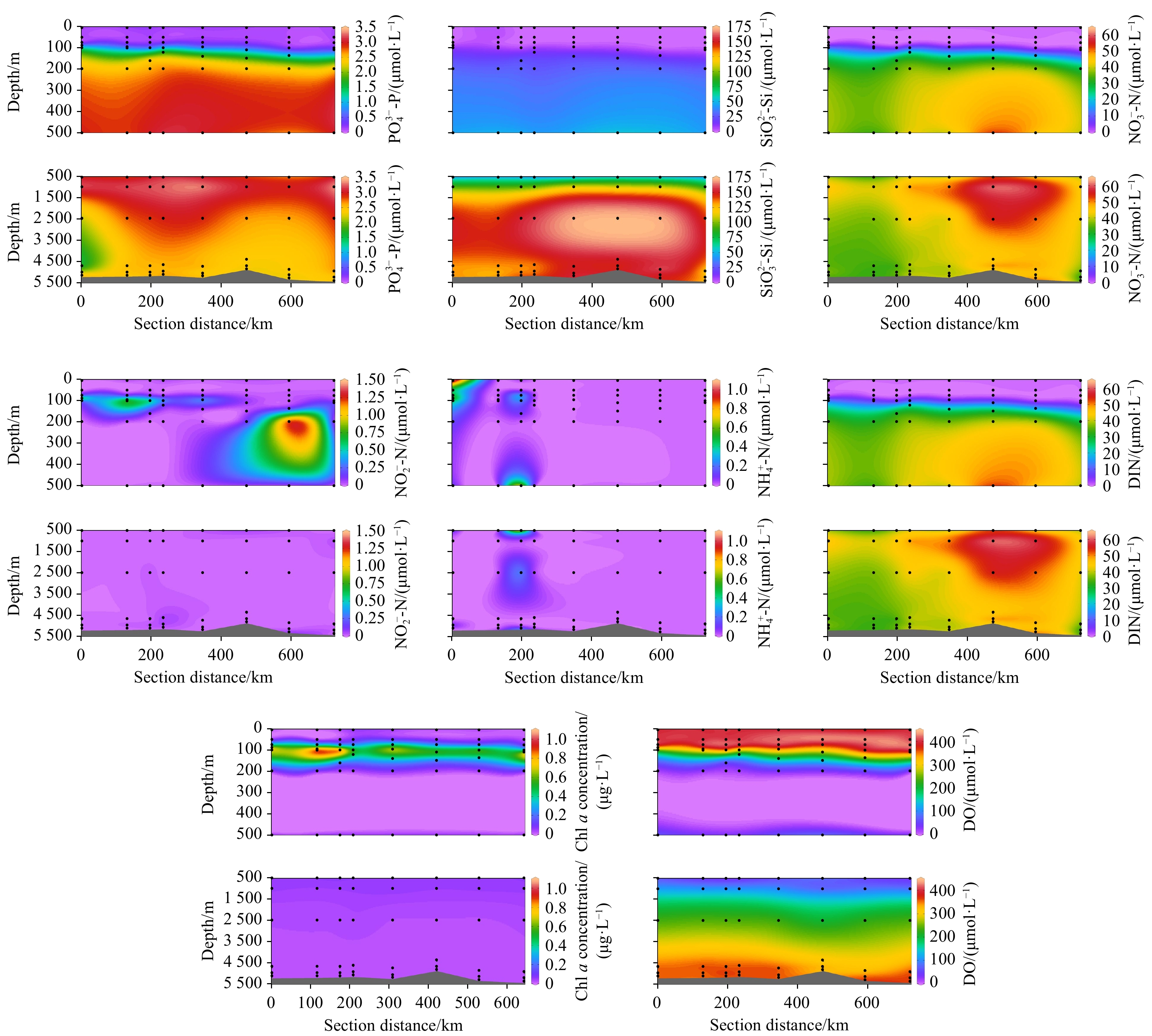
The sectional distribution of DO concentration was opposite to those of nutrient concentrations in general (Fig. 4), which was highest (more than 400 μmol/L) in the upper layer (<100 m). It decreased from about 100 m to 200−400 m, then increased from 200−400 m to the bottom (Fig. 4) with a range of 16.9−432 μmol/L and an average of 269 μmol/L. The vertical gradient of DO concentration was greatest in the layer of 80−150 m. The minimum layer of DO concentration (MLD) was located between 200 m and 400 m with the value about 10.0 μmol/L.

Figure  4.  Sectional distribution of nutrients, DO and Chl a concentration in CCFZ. These stations from left to right were the eight investigated stations from the south to the north, named CC-S01, KW1-S37, KW1-S05, KW1-S40, KW1-S01, CC-S10, CC-S09, CC-S06. These black dots aresampling sites.

DownLoad: Full-Size Img PowerPoint

This sectional distribution characteristics of DO concentration was supported by the conclusion of Tu (2006). According to previous studies, MLD in eastern tropical Pacific, lying between the pycnocline and intermediate waters, is remarkable for its size and degree of hypoxia (Kamykowski and Zentara, 1990), which is attributable to several factors: (1) high phytoplankton production; (2) a sharp permanent pycnocline that prevents local ventilation of subsurface waters; (3) a sluggish and convoluted deep circulation and therefore old ‘‘age’’ of subpycnocline waters (Fiedler and Talley, 2006). There are three major oxygen deficient zones (ODZs) in the world: the eastern tropical north Pacific (ETNP), the eastern tropical south Pacific (ETSP) and Arabian Sea (Codispoti and Christensen, 1985). And CCFZ is located in ETNP. Previous studies showed that denitrification occurs in these three major ODZs (Codispoti et al., 2001) and these regions contribute to a significant fraction of the global N₂O balance (Bange et al., 2000). Therefore, there maybe denitrification happened between 200 m and 400 m in CCFZ and associated N₂O fluxes toward the atmosphere (Chang et al., 2010). However, in this cruise, we did not sample and analyse N₂O levels in the water column. More studies are needed in the future.

3.2 Sectional distribution of nutrients

The eastern equatorial Pacific plays an important role in marine chemical cycles (Loubere, 2001), where fluxes and distributions of nutrients are controlled by interaction of circulation with biological processes. Nutrient concentrations were generally lowest in the upper layer of the ocean, which was mainly controlled by or related to biological activities, cause phytoplankton need to absorb nutrients to synthesize organic matter in the euphotic zone. The generally sectional distribution characteristics of nutrients in CCFZ were similar as follows (Fig. 4): nutrients concentration were lowest in the upper layer, which increased from the upper layer to some depths and reached the highest value, and then decreased a little until the bottom, just in accordance with previous report (Tu, 2006).

${\rm{PO}}_4^{3 - }{\text -}{\rm{P}} $ concentration in this cruise increased from upper layer to 1000 m, then it decreased a little from 1000 m to the bottom, with the range of 0.10−3.34 μmol/L and an average of 1.79 μmol/L. In the upper layer (<80 m), ${\rm{PO}}_4^{3 - }{\text -}{\rm{P}} $ concentration was generally stable and lower than 0.20 μmol/L in most stations. The vertical gradient of ${\rm{PO}}_4^{3 - }{\text -}{\rm{P}} $ concentration was greatest in the layer of 80−200 m. In 1000 m level, ${\rm{PO}}_4^{3 - }{\text -}{\rm{P}} $ concentration was highest with the value >3.30 μmol/L. ${\rm{PO}}_4^{3 - }{\text -}{\rm{P}} $ concentration showed a lower patch about 1.50 μmol/L in 4000−4500 m in the southern station (Fig. 4). Sectional distribution of ${\rm{SiO}}_3^{2 - } {\text -} {\rm{Si}} $ concentration increased from upper layer to 2500−3000 m, then it decreased a little from 2500−3000 m to the bottom. The range of ${\rm{SiO}}_3^{2 - } {\text -} {\rm{Si}} $ concentration was 0.14 μmol/L to 173.8 μmol/L with an average of 64.6 μmol/L. In the upper layer (<100 m), ${\rm{SiO}}_3^{2 - } {\text -} {\rm{Si}} $ concentration was lower than 5.00 μmol/L in most stations. The vertical gradient of ${\rm{SiO}}_3^{2 - } {\text -} {\rm{Si}} $ concentration was greatest in the layer of 100−200 m (Fig. 4). Sectional distribution of ${\rm{NO}}_3^ -{\text -} {\rm{N}}$ concentration was similar to that of ${\rm{PO}}_4^{3 - }{\text -}{\rm{P}} $ concentration, which increased from upper layer to about 1000 m with the highest value showing in Station CC-S01 in north, then it decreased from 1000 m to the bottom. The range of ${\rm{NO}}_3^ -{\text -} {\rm{N}} $ concentration was from under detection limit to 61.5 μmol/L, with an average of 24.1 μmol/L. In the upper layer (<80 m), ${\rm{NO}}_3^ -{\text -} {\rm{N}} $ concentration was stable and lower than 0.05 μmol/L in most stations. The vertical gradient of ${\rm{NO}}_3^ -{\text -} {\rm{N}} $ concentration was greatest in the layer of 80−200 m, just as that of ${\rm{PO}}_4^{3 - }{\text -}{\rm{P}} $ concentration (Fig. 4). ${\rm{NH}}_4^+ {\text - }{\rm {N}} $ concentration was generally lower than 0.03 μmol/L in the whole sectional distribution in this cruise, with the range from under detected limit to 1.05 μmol/L and an average of 0.08 μmol/L, except that there were two high patches with ${\rm{NH}}_4^+ {\text - }{\rm {N}} $ concentration about 0.80 μmol/L in surface layer in Station CC-S01 and about 0.40 μmol/L in the depth of 1000 m in Station KW1-S05, respectively (Fig. 4). ${\rm{NO}}_2^ -{\text -} {\rm{N}} $ concentration was generally lower than 0.02 μmol/L in the whole section in this cruise, with the range of 0−1.44 μmol/L and an average of 0.08 μmol/L, except that there were two high patches with ${\rm{NO}}_2^ -{\text -} {\rm{N}} $ concentration about 0.60 μmol/L in 100 m layer in Station KW-S07 and 1.20 μmol/L in the depth of 200 m in Station CC-S09, respectively (Fig. 4). As ${\rm{NO}}_3^ -{\text -} {\rm{N}} $ was the main form of DIN (dissolved inorganic nitrogen; ${\rm{NH}}_4^+{\text -} {\rm{N}} +{\rm{NO}}_3^ -{\text -} {\rm{N}}+{\rm{NO}}_2^ -{\text -} {\rm{N}} $), the sectional distribution of DIN concentration was just as that of ${\rm{NO}}_3^ -{\text -} {\rm{N}} $ concentration, which increasing from upper layer to about 1000 m, then it decreased from 1000 m to the bottom. The range of DIN concentration was from under detection limit to 61.5 μmol/L, with an average of 25.7 μmol/L. In the upper layer (<80 m), DIN concentration was stable and lower than 0.50 μmol/L in most stations. The vertical gradient of DIN concentration was greatest in the layer of 80−200 m too. The highest patch of DIN concentration was showing at about 1000 m in Station CC-S01 in north of this investigation area (Fig. 4).

Furthermore, the uniform upper layer gradually became shallow from southern stations to northern ones (Fig. 4). And the study area has a shallow mixing layer and a thin thermocline. In the vertical direction, the water column has obvious stratification phenomenon (Tu, 2006).

3.3 Comparing nutrient concentrations and ratios with those in other areas

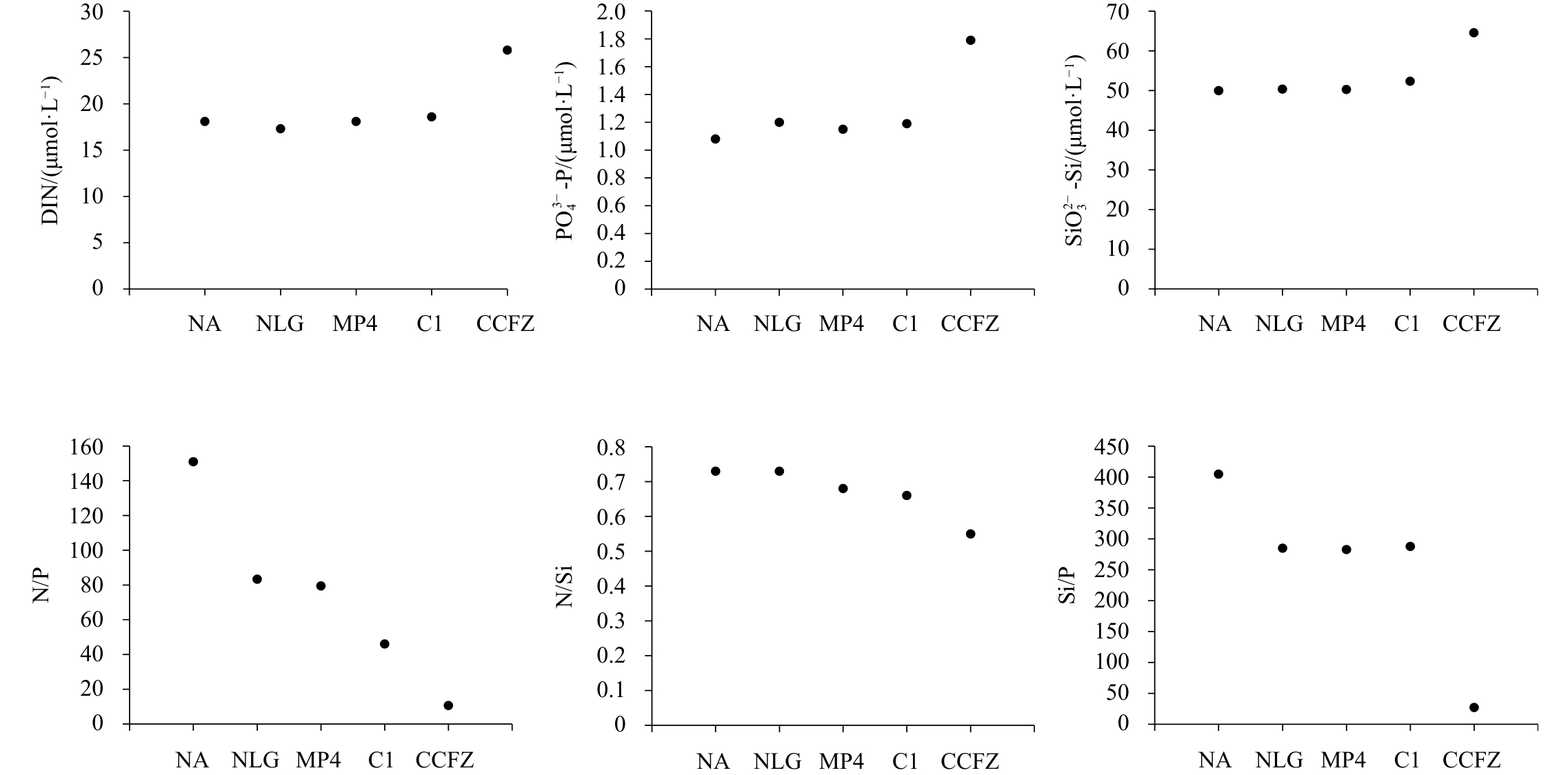
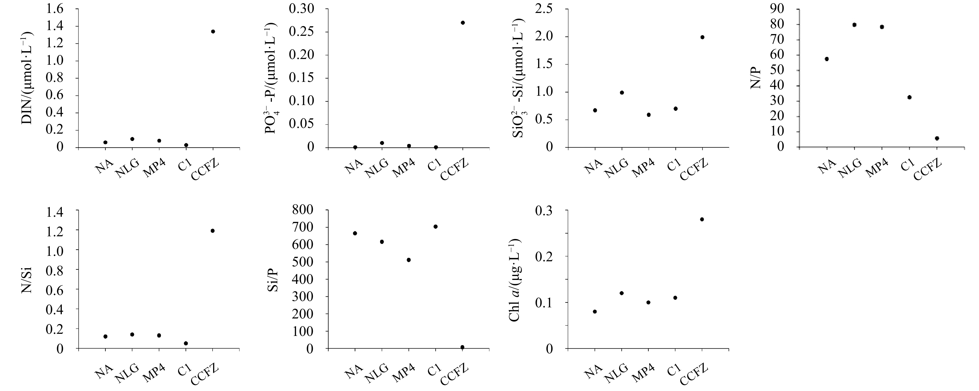
During July to August in 2017, a cruise was carried out in three seamounts (ie., the seamounts Demao Guyot and Batiza Guyot (NA), Niulang Guyot (NLG) and McDonnell Guyot (MP4), respectively) and a untitled sea basin (named C1) in the subtropical western Pacific Ocean (SWPO) by Third Institute of Oceanography, Ministry of Natural Resources of China (unpublished data) with same methods of sampling and analysis (General Administration of Quality Supervision, Inspection and Quarantine of the People’s Republic of China and Standardization Administration, 2008). Comparing nutrient concentrations in SWPO and CCFZ (Tables 4 and 5, Figs 5 and 6), it could be concluded that both in the whole water column and euphotic zone (0−100 m), concentrations of DIN, ${\rm{PO}}_4^{3 - }{\text -}{\rm{P}} $ and ${\rm{SiO}}_3^{2 - } {\text -} {\rm{Si}} $ were much higher in CCFZ than those in SWPO especially in euphotic zone. Tu (2006) also concluded that DIN and ${\rm{PO}}_4^{3 - }{\text -}{\rm{P}} $ concentration was higher in CCFZ than those in Station ALOHA in the North Pacific (Karl, 2001) and Station S1 in the South China Sea (Wu et al., 2003), comparable to Station BATS in the North Atlantic (Cavender-Bares et al., 2001), however lower than those in the equatorial Pacific Ocean (Tu, 2006). The spatial and temporal distribution of nutrients are mainly influenced by the absorption of phytoplankton community, the regeneration and transport process of nutrients (Raimbault et al., 1999). And physical process is important factor controlling nutrients transport in horizontal and vertical directions. CCFZ is located at the northeast of equatorial Pacific Ocean, between the junction of North Equatorial Current and North Equatorial Countercurrent. In July to September, north of 9.5°N is mainly controlled by western North Equatorial Current, and south of it is mainly controlled by eastern North Equatorial Countercurrent (Tu, 2006). In this cruise, most stations were located at north of 9.5°N (Fig. 1 and Table 1), therefore the study area is mainly controlled by western North Equatorial Current, which might bring water mass from the east with higher nutrient concentrations produced by coastal upwelling in equatorial Pacific upwelling or Peru upwelling (Feely et al., 1987; Tu, 2006). Furthermore, according to conclusions of Toggweiler and Carson (1995), the accumulation of nitrate in the Eastern Equatorial Pacific is a property of the regional ecosystem, where nutrients are regenerated efficiently within the water column and the circulation system operates as a nutrient trap to concentrate them. Therefore, nutrient concentrations in waters of the study area were generally higher than other areas in the North Pacific including seamounts in SWPO and Station ALOHA, because the nutrients were supplemented not only from vertical direction brought up from deep water, but also from horizontal direction transported from the equatorial Pacific, and also from regenerated within the water column and so on. And this conclusion was consistent with previous research (Feely, 1987; Fiedler and Talley, 2006).

Table  4.  Comparing nutrient concentrations and molar ratios in water columns in SWPO and CCFZ in 2017

Area		DIN/(μmol·L−1)	${\rm{PO}}_4^{3 - }{\text -}{\rm{ P}} $/(μmol·L−1)	${\rm{SiO}}_3^{2 - } {\text -} {\rm{Si}} $/(μmol·L−1)	N/P	N/Si	Si/P
NA	range	nd−56.8	nd−2.91	0.29−208	1.21−2284	0.00−2.90	11.6−1372
	average	18.1±20.8	1.08±1.27	50.0±63.5	151±392	0.73±0.73	405±419
NLG	range	nd−46.1	nd−2.93	0.36−145	0.94−1157	0.01−2.90	10.8−1784
	average	17.3±18.6	1.20±1.27	50.4±59.5	83.4±182	0.73±0.76	285±433
MP4	range	nd−46.3	nd−2.91	0.31−153	0.50−956	nd−3.00	8.57−1166
	average	18.1±20.1	1.15±1.27	50.3±61.6	79.5±162	0.68±0.71	283±353
C1	range	0.02−42.8	nd−2.75	0.50−140	13.6−106	0.04−1.75	21.9−1114
	average	18.6±19.5	1.19±1.25	52.4±60.4	46.1±25.3	0.66±0.57	288±385
CCFZ	range	nd−61.5	0.10−3.34	0.14−174	0.01−21.7	0.00−3.09	1.05−80.0
	average	25.8±19.3	1.79±1.17	64.6±63.0	10.7±6.64	0.55±0.50	27.3±23.2
Note: nd represents under detection limit.

 | Show Table

DownLoad: CSV

Table  5.  Comparing nutrient concentrations, nutrient molar ratios, and Chl a concentration in 0−100 m depth layer of SWPO and CCFZ in 2017

Area		DIN/(μmol·L−1)	${\rm{PO}}_4^{3 - }{\text -}{\rm{ P}} $/(μmol·L−1)	${\rm{SiO}}_3^{2 - } {\text -} {\rm{Si}} $/(μmol·L−1)	N/P	N/Si	Si/P	Chl a/(μg·L−1)
NA	range	nd−0.44	nd	0.29−1.01	0.54−442	0.00−0.89	286−1007	nd−0.17
	average	0.06±0.11	nd±0.00	0.67±0.21	57.6±108	0.12±0.24	666±208	0.08±0.05
NLG	range	0.01−0.52	nd−0.10	0.36−1.61	0.43−523	0.01−1.47	11.7−1611	nd−0.39
	average	0.10±0.13	0.01±0.02	0.99±0.35	79.8±132	0.14±0.30	617±456	0.12±0.10
MP4	range	nd−0.43	nd−0.05	0.36−0.87	0.54−432	0.00−0.54	10.9−867	nd−0.32
	average	0.08±0.12	0.00±0.01	0.59±0.17	78.4±127	0.13±0.16	512±244	0.10±0.09
C1	range	0.02−0.05	nd	0.50−1.01	19.5−48.0	0.02−0.10	495−1007	0.05−0.19
	average	0.03±0.01	nd±0.00	0.70±0.22	32.6±13.1	0.05±0.03	704±219	0.11±0.06
CCFZ	range	0.00−12.4	0.10−1.11	0.14−8.73	0.00−29.3	0.00−9.10	1.05−40.4	0.01−1.02
	average	1.34±2.75	0.27±0.24	1.99±2.16	5.79±7.61	1.19±2.22	7.36±6.98	0.28±0.30
Note: nd represents under detection limit.

 | Show Table

DownLoad: CSV

Figure  5.  Average of nutrient concentrations and molar ratios in SWPO and CCFZ in 2017.

DownLoad: Full-Size Img PowerPoint

Figure  6.  Average of nutrient and Chl a concentrations in 0−100 m depth layer of SWPO and CCFZ in 2017

DownLoad: Full-Size Img PowerPoint

Comparing nutrients ratios in SWPO and this study area (Tables 4 and 5, Figs 5 and 6), it could be concluded that P was the main limited nutrient in SWPO, however in CCFZ, N limited the growth of phytoplankton especially in euphotic zone. Under the condition of N limitation, phytoplankton can use total organic nitrogen as nitrogen source for its growth (Libby and Wheeler, 1997), and Ni (2011) reported that total organic nitrogen accounting more than 75% of total nitrogen in this study area.

3.4 Comparing nutrient concentrations between investigations in 1998-2003 and in 2017

In 1991, the application of China Ocean Committee (COM) as a pioneer investor in polymetallic nodules was approved by the ISA. To implement obligation and responsibility to investigate and study the possible environmental impact of mining activities, the COM promoted an investigation about baseline and natural changes in Chinese contract area in CCFZ in 1998−2003, including the baseline characteristics of spatial distribution of nutrients (Tu, 2006). In 2017, the TIO again carried out this cruise to study the environmental conditions in this area. The results of changes of nutrient concentrations in this 20 years are showed in Table 6. In the investigation in 1998−2003, ${\rm{NO}}_3^ -{\text -} {\rm{N}}$ concentration was almost lower than 0.05 μmol/L in the surface layer (<20 m) except that in 2001 (Table 6), then it increased with the depth till 800 m with highest value there. And from 800 m to the bottom, ${\rm{NO}}_3^ -{\text -} {\rm{N}} $ concentration decreased a little with the depth (Tu, 2006). In this study, ${\rm{NO}}_3^ -{\text -} {\rm{N}} $ concentration was lower than 0.05 μmol/L in the upper layer (<80 m) (Fig. 4), then it increased with the depth till 1000 m with highest value there. And from 1000 m to the bottom, ${\rm{NO}}_3^ -{\text -} {\rm{N}} $ concentration decreased a little with the depth. It could be concluded that in this 20 years, the sectional distribution characteristics of ${\rm{NO}}_3^ -{\text -} {\rm{N}} $ concentration was almost the same. Furthermore, the highest value of ${\rm{NO}}_3^ -{\text -} {\rm{N}} $ concentration decreased from about 64 μmol/L in 1998−1999, to 52 μmol/L in 2001−2003, and to 50 μmol/L in 2017. In the previous study, ${\rm{NO}}_2^ -{\text -} {\rm{N}} $ concentration showed highest patch in 50−100 m (Tu, 2006), however in this study, ${\rm{NO}}_2^ -{\text -} {\rm{N}} $ concentration showed highest patch in about 100−500 m (Fig. 4). ${\rm{NH}}_4^+ {\text - }{\rm {N}} $ concentration did not change a lot in vertical direction in 1998−2003, and it was the main form of DIN for the growth of phytoplankton community in the surface layer. However in 2017, ${\rm{NH}}_4^+ {\text - }{\rm {N}} $ concentration was almost under detection in most study areas except some small patches in southern stations (Fig. 4). And the range of ${\rm{NO}}_2^ -{\text -} {\rm{N}} $ and ${\rm{NH}}_4^+ {\text - }{\rm {N}} $ concentration changed a little in this 20 years. And ${\rm{NO}}_3^ -{\text -} {\rm{N}} $ was the main form of DIN in this study area. In the previous reports, the sectional distribution of ${\rm{PO}}_4^{3 - }{\text -}{\rm{P}} $ concentration was just like that of ${\rm{NO}}_3^ -{\text -} {\rm{N}} $ concentration. ${\rm{PO}}_4^{3 - }{\text -}{\rm{P}} $ concentration was almost lower than 1 μmol/L in the surface layer (<20 m), then it increased with the depth till 800 m too (Tu, 2006). In this study, ${\rm{PO}}_4^{3 - }{\text -}{\rm{P}} $ concentration was lower than 0.5 μmol/L in the upper layer (<80 m), then it increased with the depth till 1000 m with highest value there (Fig. 4). And from 1000 m to the bottom, ${\rm{PO}}_4^{3 - }{\text -}{\rm{P}} $ concentration decreased a little with the depth, which was also just similar to the sectional distribution of ${\rm{NO}}_3^ -{\text -} {\rm{N}} $ concentration. In both investigations in 1998−2003 and 2017, ${\rm{SiO}}_3^{2 - } {\text -} {\rm{Si}} $ concentration increased with the depth till 3000 m, showing highest value there, and decreased a little from 3000 m to the bottom (Tu, 2006).

Table  6.  Ranges of nutrient and DO concentrations (μmol/L) in CCFZ in 1998−2017 (Tu, 2006)

Sampling time	${\rm{PO}}_4^{3 - }{\text -}{\rm{ P}} $	${\rm{SiO}}_3^{2 - } {\text -} {\rm{Si}} $	${\rm{NO}}_3^ - {\text -} {\rm{N}} $	${\rm{NO}}_2^ - {\text -} {\rm{N}} $	${\rm{NH}}_4^+ {\text - }{\rm {N}} $	DO
Aug. 1998	0.07−3.09	0.00−165.9	0.00−64.12	0.00−0.85	0.00−2.04	32.8−440.2
Oct. 1999	0.00−3.28	0.00−178.3	0.00−64.35	0.01−1.58	−	28.8−438.9
Oct. 2001	0.02−3.19	0.40−152.8	0.13−54.15	0.00−0.73	0.49−1.07	22.4−442.4
Sept. 2002	0.10−3.10	0.62−133.9	0.01−50.31	−	−	44.5−426.3
Sept.−Oct. 2003	0.05−3.22	2.94−152.8	0.00−52.56	0.00−0.54	−	15.0−457.5
Aug.−Oct. 2017	0.11−3.34	0.14−172.0	0.00−49.77	0.00−0.99	0.00−1.05	16.9−424.6
Note: − represents no data.

 | Show Table

DownLoad: CSV

3.5 Sectional distribution of Chl a in euphotic zone and its controlling factors

The direct reason of nutrients deficiency in euphotic zone especially in the upper layer of oceans is the absorption by phytoplankton (Tu, 2006). In this study area, Chl a concentration ranged from 0.01 μg/L to 1.02 μg/L in euphotic zone (0−100 m), with an average of 0.28 μg/L. The sectional distribution of Chl a concentration increased from surface to about 100 m, where the subsurface chlorophyll maximum (SCM) was located, with the highest value occurring at central stations of southern region in this study area (Fig. 4). Then with the limitation of light, Chl a concentration decreased from 100 m to about 150 m, where Chl a concentration was under detection limit again (Fig. 4). In the upper layer (<50 m), Chl a concentration was almost <0.10 μg/L. And the depth of SCM increased from southern stations to northern ones (Fig. 4), which was also supported by previous research (Tu, 2006). Study found that light and nutrients together control SCM in oceans (Bahamón et al., 2003). In this study area, N was the main limited nutrient to phytoplankton growth, and nitrate was the main form of dissolved inorganic nitrogen (Fig. 4). It could be found that SCM located near nitracline, this phenomenon was recorded in the tropical Atlantic Ocean by Bahamón et al. (2003) too.

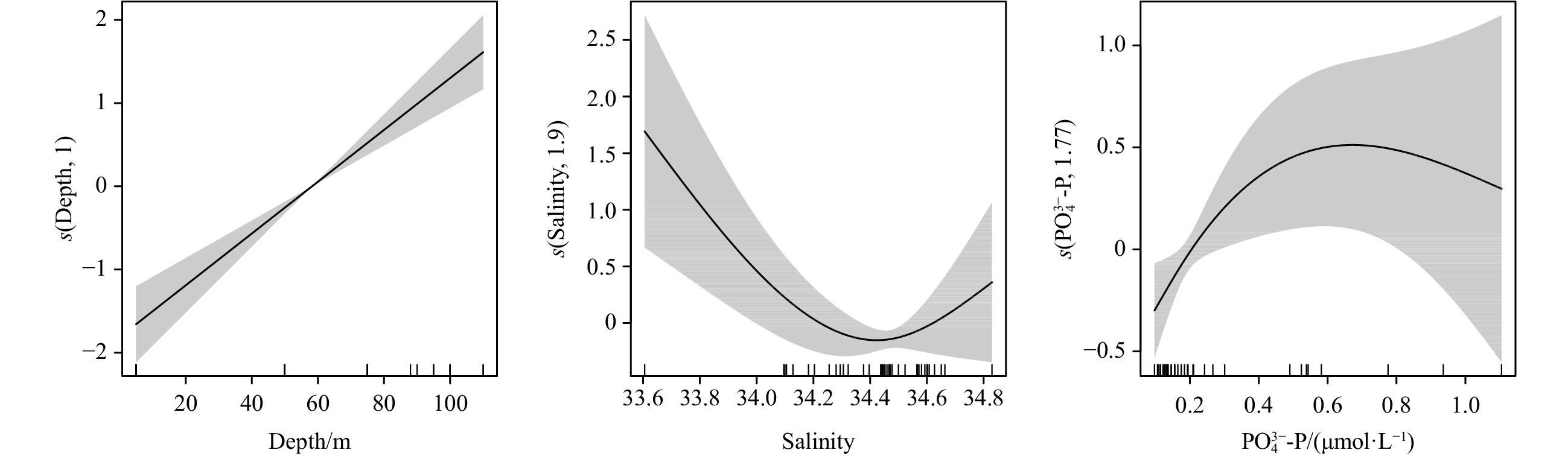
To study how environmental factors especially light and nutrients control the biomass of phytoplankton community, this paper used a model named GAMs to analysis the bottom-up process. In marine science, GAMs have been used in modeling phytoplankton biomass (Deng et al., 2015; Song et al., 2014; Zhou et al., 2014; Raitsos et al., 2012; Kim et al., 2019). GAMs allow the effects of individual environmental parameters to be examined and the underlying controlling mechanisms being inferred (Chen et al., 2012). To discuss how environmental parameters especially nutrient concentrations affect Chl a concentration by bottom-up process, environmental factors including of temperature, salinity, depth, DIN, ${\rm{PO}}_4^{3 - }{\text -}{\rm{P}} $, ${\rm{SiO}}_3^{2 - } {\text -} {\rm{Si}} $, N/P, N/Si, Si/P and DO were selected to be independent variables, and Chl a to be dependent variable from surface to SCM in euphotic zone in this study area (0−100 m). In the process of application of GAMs, concurved linearity is a common problem that can not be ignored. Generally, when there is a definite collinearity relationship between the prediction variables in the model, the concurved linearity must also exist among these variables (Jia et al., 2005). In this study, we used variance inflation factor (VIF) to judge concurved linearity of environmental parameters (Deng et al., 2015). Experience shows that, when 0< VIF<10, there is no multicollinearity; when 10≤VIF<100, there is strong multicollinearity; when VIF≥100, there is serious multicollinearity. Table 7 shows the VIF of each independent variable (Deng et al., 2015). Then we delete parameter of ${\rm{SiO}}_3^{2 - } {\text -} {\rm{Si}} $ with the highest VIF (>10) and figure out VIF of other parameters until all reserved ones with VIF<10. It shows that concentrations of DIN and ${\rm{SiO}}_3^{2 - } {\text -} {\rm{Si}} $ have strong multicollinearity with other parameters. After delete concurved linearity of parameters of DIN and ${\rm{SiO}}_3^{2 - } {\text -} {\rm{Si}} $, this study used approximate significance of smooth terms with lgChl a to ensure each parameters in the model was significant. Figure 7 showed functional relationship between lgChl a and individual significant parameter in this study. Depth, salinity and ${\rm{PO}}_4^{3 - }{\text -}{\rm{P}} $ concentration were major factors controlling the growth of phytoplankton community (Fig. 7 and Table 8). lgChl a almost showing a positive correlation with depth from surface to about 100 m, which was consistent with the conclusion above that the sectional distribution of Chl a concentration increased from surface to about 100 m (Fig. 4). lgChl a increased with ${\rm{PO}}_4^{3 - }{\text -}{\rm{P}} $ concentration from 0.10 μmol/L to 0.60 μmol/L, then decreased a little with ${\rm{PO}}_4^{3 - }{\text -}{\rm{P}} $ from 0.60 μmol/L to 1.00 μmol/L. However when ${\rm{PO}}_4^{3 - }{\text -}{\rm{P}} $ concentration >0.60 μmol/L, the confidence interval was much larger making the decrease of credibility (Fig. 7). Sectional distribution of ${\rm{PO}}_4^{3 - }{\text -}{\rm{P}} $ concentration increased from surface to 1000 m and Chl a concentration showed the highest value at about 100 m which was co-limited by nutrients and light. Furthermore, nutrients are crucial to phytoplankton growth, but variations in Chl a concentrations and phytoplankton community compositions indicate that different algal species require different nutrients. lgChl a showed negative relationship with S from about 33.6 to 34.4, then increased with S afterwards. Just like what mentioned above, the sectional distribution of S in euphotic zone was quite complicated in CCFZ.

Table  7.  Variance inflation factor (VIF) among parameters in CCFZ in 2017

	Depth	Temperature	Salinity	DO	DIN	${\rm{PO}}_4^{3 - }{\text -}{\rm{ P}} $	${\rm{SiO}}_3^{2 - } {\text -} {\rm{Si}} $	N/P	N/Si	Si/P
Initial	6.59	10.18	2.63	9.38	31.88	35.45	64.36	14.58	4.53	13.42
Ultimate	6.51	9.32	2.61	7.54	−	8.48	−	7.84	3.68	1.16
Note: − represents no data.

 | Show Table

DownLoad: CSV

Figure  7.  Generalized Additive Models (GAMs) plots illustrate significant relationship (p<0.05) between the lgChl a and depth, salinity and ${\rm{PO}}_4^{3 - }{\text -}{\rm{P}} $. The solid line is the fitted line, while the shaded areas represent 95% confidential intervals. The numbers in the labels of y-axis denote the effective degrees of freedom; the definition of the labels of y-axis refers to Table 8.

DownLoad: Full-Size Img PowerPoint

Table  8.  Statistical results of GAMs in CCFZ in 2017

Model	R2	GCV	n
lgChl a=s(depth)+s(salinity)+s(${\rm{PO}}_4^{3 - }{\text -}{\rm{P}} $)+b	0.863	0.280	41
Note: R2 represents the adjusted proportion of total variability explained by the model; GCV, generalized cross validation score; n, the total number of samples; s, thin plate regression spline; b, a mean constant.

 | Show Table

DownLoad: CSV

4. Conclusions

(1) Dissolved inorganic nutrient (N, P and Si) concentrations in CCFZ were lowest in the upper layer, and increased from surface to some depth, then decreased a little to the bottom. N was the limited nutrient factor for the growth of phytoplankton community in this area.

(2) The sectional distribution of DO concentration was opposite to those of nutrient concentrations in general.

(3) Nutrient concentrations and molar ratios have no obvious changes in 2017 comparing with those in the investigation in 1998−2003.

(4) Nutrient concentrations in the study area was higher than those in the seamounts and Station ALOHA in the North Pacific, because they were supplemented from the equatorial Pacific with high nutrients, and also from regenerated within the water column themself.

(5) Depth, salinity and ${\rm{PO}}_4^{3 - }{\text -}{\rm{ P}} $ concentration were major factors controlling the growth of phytoplankton community.