


Figure
1.
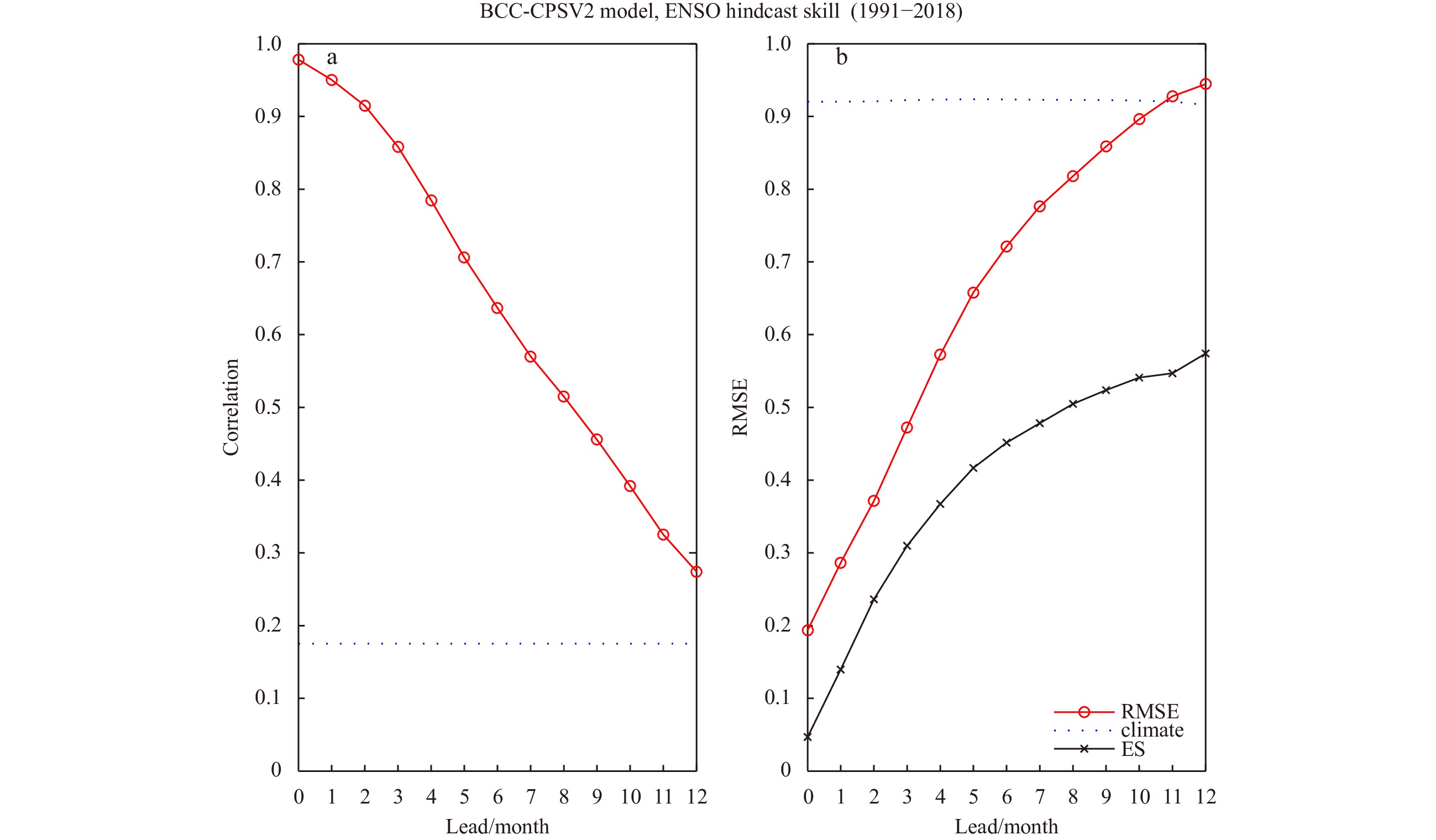
The correlation skill, RMSE and ensemble spread (ES) of the BCC-CPS2 model as function of lead month.
| Citation: | Yanjie Cheng, Youmin Tang, Tongwen Wu, Xiaoge Xin, Xiangwen Liu, Jianglong Li, Xiaoyun Liang, Qiaoping Li, Junchen Yao, Jinghui Yan. Investigating the ENSO prediction skills of the Beijing Climate Center climate prediction system version 2[J]. Acta Oceanologica Sinica, 2022, 41(5): 99-109. doi: 10.1007/s13131-021-1951-7

|
El Niño-Southern Oscillation (ENSO), which occurs in the tropical Pacific Ocean over a period of 2–7 years, results in the strongest inter-annual climatic variability across the globe. It has significant impacts on global climate, ecology, and society. Accurate ENSO predictions are able to assist in the management of natural resources and the environment. Over the past decades, significant progress has been made in the understanding and prediction of ENSO events. Many ENSO prediction models of varying complexity levels are currently being applied to issue routine predictions, including statistical, dynamical, hybrid coupled and fully coupled general circulation models. The majority of such models can achieve a correlation skill of 0.5 for 6–12 month predictions (e.g., see IRI online at
The performance of individual models depends strongly on season and ENSO phase and intensity (e.g., Jin et al., 2008; Sohn et al., 2016). In particular, ENSO is better predicted in (1) strong events; (2) warm and cold growth phases compared to their corresponding decay phases; (3) seasons distinct to boreal spring, which is the so-called “Spring Predictability Barrier” (SPB) (Latif et al., 1994; McPhaden, 2003). These features can be approximately interpreted in a uniform signal and noise-based framework, as reported in intermediate and coupled General Circulation Models (GCMs) (e.g., Tang et al., 2005; Cheng et al., 2010; Kumar and Hu, 2014; Kumar et al., 2017; Hu et al., 2019; Tian et al., 2019).
Despite the extensive number of models (intermediate, hybrid, fully coupled) adopted to investigate ENSO predictability, research on the application of operational seasonal forecast models to study ENSO predictability, and in particular, on potential predictability, is limited. Tian et al. (2019) suggested that the seasonality of tropical SST variability may fundamentally contribute to the ENSO SPB according to the results from Coupled Model Intercomparison Project Phase 5 (CMIP5) models. Hu et al. (2019) employed the Climate Forecast System version 2 (CFSv2) operational model to explore the predictability source, demonstrating the dominance of the ENSO signal in the ENSO prediction skill. They also revealed that the ensemble spread, which often represents the noise component, exhibits a minimal dependence on the ENSO amplitude. Their results suggest that model initial error growth may have limited influence on prediction skill during the ENSO transition phase, because during those periods the signal or amplitude of SSTA to be predicted is weak.
It is helpful to further investigate ENSO predictability using more operational seasonal prediction models. For this purpose, we evaluated ENSO predictability for the BCC-CPS2 for the period from 1990 to 2018. BCC-CPS2 (originally denoted BCC_CSM1.1m, Wu et al., 2008, 2014) is the current operational seasonal prediction system of the Beijing Climate Center in China.
Recently, Ren et al. (2020) gives a review of ENSO prediction methods and related applications conducted by Chinese researchers. For the BCC-CPS2, the ENSO correlation prediction skill was examined for the time period of 1996–2015 in Ren et al. (2017), with Ni
The rest of this paper is organized as follows. Section 2 briefly introduces the BCC_CPS2 model and its initial perturbation methods. Section 3 outlines the deterministic and probabilistic skill metrics employed for the evaluation of ensemble predications. Sections 4 and 5 present the actual and potential prediction skills respectively; and Section 6 details the signal/noise dependence of the prediction skill. Section 7 concludes the paper.
The BCC-CPS2 (Beijing Climate Center (BCC) Climate Prediction System Version 2) is a moderate resolution version of BCC Climate System Model version 1.1 (Wu et al., 2008, 2014). The atmospheric component is BCC_AGCM2.2 at T106 horizontal resolution and 26 vertical hybrid sigma/pressure levels. The land processes adopt the schemes from the BCC Atmosphere and Vegetation Interaction Model, version 1.0 (BCC_AVIM1.0) with a same horizontal resolution as the atmospheric model. The ocean component of BCC_CSM1.1(m) introduces the modules from the Geophysical Fluid Dynamics Laboratory Modular Ocean Model, version 4, with 40 levels (MOM4-L40, Griffies et al., 2005) with the sea ice component from the Sea Ice Simulator (SIS, Winton, 2000). Both the ocean and sea ice models use a tri-polar grid, in which the latitudinal resolution is 1° longitude and the meridional resolution ranges from (1/3)° latitude between 10°S and 10°N to 1° latitude at 30°S/30°N poleward. The atmospheric initial values are initialized from the four-time daily NCEP-NCAR R1 data, and the oceanic initial values from the ocean temperature of the Global Oceanic Data Assimilation System (GODAS), using a nudging scheme with a timescale of three days.
All of these components are coupled without flux adjustment. The BCC-CPS2 is initialized by GODAS SST and NCEP atmospheric fields on the first day of each calendar month and then runs forward over 12 months during 1991–2018. Each experiment has 24 ensemble members.
Hoffman and Kalnay (1983) proposed the lagged average forecast (LAF) method for initial perturbation used in ensemble prediction, which has been widely used in weather and climate ensemble prediction systems. In the BCC_CPS2 model, the LAF method has been employed for the operational and seasonal forecast to generate atmospheric and oceanic initial perturbations with 15 ensemble members. In addition, an empirical climate-related singular vector (SV) (Kleeman et al., 2003; Tang et al., 2006) was also applied to SSTA to generate 9 ensemble members for ocean initial perturbation. More detailed procedure for obtaining SV is illustrated in Kleeman et al. (2003) and Tang et al. (2006).
Correlation-based skill and RMSE-based skill are used to measure deterministic prediction skill. The overall skill of ensemble mean predictions over the 29 years is measured by anomaly correlation (R) and root mean square error (RMSE). The observed SST dataset over the time period is NOAA OISST dataset (
The Brier score (BS; e.g., Wilks, 2006) is a commonly used verification measure for assessing the accuracy of probability forecasts. It is the mean squared error between the forecast probability and the observed frequency over the verification period.
| $$ BS = \frac{1}{N}\sum\limits_{i = 1}^N {{{\left( {{P_i} - {O_i}} \right)}^2}} , $$ | (1) |
where N is the number of total verification samples (N=348 here), Pi is the forecast probability and Oi is a value 1 or 0 depending on whether the event occurred or not. Similar to the deterministic prediction skill RMSE, a smaller BS indicates a better forecast.
The BS can be decomposed into three items: reliability (REL), resolution (RES), and uncertainty (UNC) as follows (e.g., Wilks, 2006):
| $$ \begin{gathered} {\rm{BS}} = {{\dfrac{1}{N}\sum\limits_{k = 1}^{K = 10}{{n_k}} {{({P_{{\rm{f}}k}} - {P_{\rm{o}}}_k)}^2}}}- \ {{\dfrac{1}{N}\sum\limits_{k = 1}^{K = 10}{{n_k}} {{({P_\rm{o}}_k - s)}^2}}} + {{s(1 - s)}} . \hfill\\ \begin{array}{*{20}{c}}{}&{}&{}&{}&{}&{{\text{REL}}}&{}&{}&{}&{}&{}&{}&{}&{{\text{RES}}} &{}&{}&{}&{{\text{UNC}}} \end{array} \hfill \\ \end{gathered} $$ | (2) |
Over the verification period, the observed frequency of occurrence Po can be partitioned into K bins (K=10 in this study) according to the forecast Pf. Pfk is the averaged forecast probability at bin k.
A good Brier score occurs at a large RES item and a small REL, corresponding a high resolution and good reliability. The ideally perfect RES value equals to the uncertainty item UNC that gives the upper limit of the predictability of the probabilistic prediction system.
In order to compare the Brier score to that for a reference forecast system BSref , it is convenient to define the Brier skill score (BSS; Wilks, 2006).
| $$ {\text{BSS}} = 1 - \frac{{{\text{BS}}}}{{{\text{B}}{{\text{S}}_{{\text{ref}}}}}}. $$ | (3) |
If the climatological forecast is taken as reference prediction,
With Eq. (2), Eq. (3) can be rewritten as follows:
| $$ {\text{BSS}} = \frac{{{\text{RES}}}}{{{\text{UNC}}}} - \frac{{{\text{REL}}}}{{{\text{UNC}}}} = {B_{{\text{res}}}} - {B_{{\text{rel}}}}, $$ | (4) |
where
Ensemble mean (EM or
| $$ {\mu _{\rm{p}}}(i,t) = \frac{1}{M}\sum\limits_{m = 1}^{M = 24} {{T_{\rm{p}}}(i,t,m)}, $$ | (5) |
| $$ {\sigma _{\rm{p}}}(i,t) = \sqrt {\frac{1}{{M - 1}}\sum\limits_{m = 1}^M {{{({T_{\rm{p}}}(i,t,m) - {\mu _{\rm{p}}}(i,t))}^2}} }, $$ | (6) |
| $$ {\lambda _{\rm{p}}}(i,t) = \left| {\frac{{{\mu _{\rm{p}}}(i,t)}}{{{\sigma _{\rm{p}}}(i,t)}}} \right|, $$ | (7) |
where Tp is the index of Ni
Note that instead of using EM, the square of ensemble mean, denoted by EM2 or
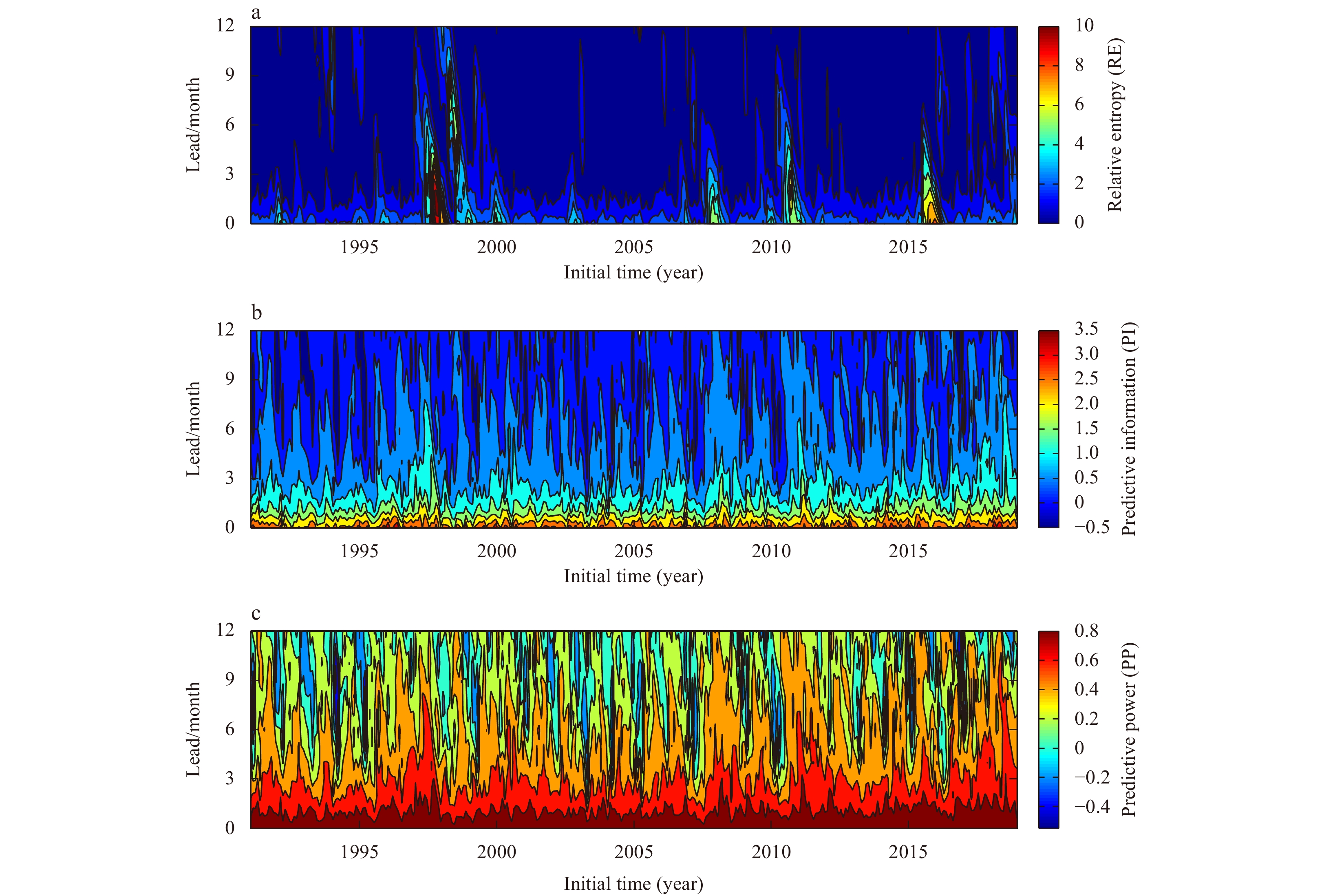
The definition of the information-based measures of potential predictability are based on information theory which can be found in relevant literature (e.g., DelSole, 2004; DelSole and Tippttt, 2007; Kleeman, 2002; Tang et al., 2008). For practical application, relative entropy (RE), predictive information (PI), and predictive power (PP) can be simplified as (DelSole, 2004; Cheng et al., 2011):
| $$ {\rm{PI}} = \frac{1}{2}\ln \left( {\frac{{\sigma _{\rm{q}}^2}}{{\sigma _{\rm{p}}^2}}} \right) , $$ | (8) |
| $$ \begin{gathered} {\rm{RE}} = \frac{1}{2}\left[ {\underline {\ln \left( {\frac{{\sigma _{\rm{q}}^2}}{{\sigma _{\rm{p}}^2}}} \right) + \frac{{\sigma _{\rm{p}}^2}}{{\sigma _{\rm{q}}^2}} - 1} + \underline{\underline {\frac{{\mu _{\rm{p}}^2}}{{\sigma _{\rm{q}}^2}}}} } \right] = {\rm{PI}} + \frac{1}{2}\left[ {\frac{{\sigma _{\rm{p}}^2}}{{\sigma _{\rm{q}}^2}} - 1 + \frac{{\mu _{\rm{p}}^2}}{{\sigma _{\rm{q}}^2}}} \right] \hfill \\ \begin{array}{*{20}{c}} {}& {}&{}&{}&{{\rm{dispersion}}\begin{array}{*{20}{c}} {\begin{array}{*{20}{c}} {} \end{array}}&{}&{{\rm{signal}}} \end{array}} \end{array} \hfill \\ \end{gathered} , $$ | (9) |
| $$ {\rm{PP}} = 1 - {\left( {\frac{{\sigma _{\rm{p}}^2}}{{\sigma _{\rm{q}}^2}}} \right)^{1/2}} , $$ | (10) |
where the variance
The ENSO ensemble prediction skill of the BCC-CPS2 model is evaluated using the traditional deterministic skill metrics, including R and RMSE, together with probabilistic skill measures such as the Brier Skill Score (BSS) and its two components (reliability score REL and resolution score RES).
Figure 1a presents the correlation skill of the BCC model as a function of lead month. The dash-line 0.175 is the threshold at the T-test significant level of 0.001. The results suggest the ability of the BCC model to capture ENSO phase variations approximately 12 months ahead. The RMSE and ensemble spread (ES) are presented in Fig. 1b, along with the climatological standard deviation of the observed Ni
Probabilistic skill metrics are used to evaluate the probabilistic properties of an ensemble prediction system. Figure 2 presents the BSS score and its two components REL and RES for the cold, warm, and neutral states of ENSO across the lead month. For BSS>0, the prediction is more useful than the climate prediction. The left panel demonstrates that the warm and the cold ENSO states contain useful information at around 9–11 lead months, while only 6 months of useful information is observed at the neutral ENSO states. Note that the reliability score is defined as a negative oriented score, implying that a perfect reliable ensemble scheme has a zero REL score value. The REL is associated with the ensemble spread. The center panel of Fig. 2 demonstrates the RELs at the three ENSO phase states are lower than 0.15 at the lead months of 0–9. This indicates that the ensemble construction scheme of BCC-CPS2 is acceptable, otherwise a large reliability score would contribute negatively to the BSS score; for example, the negative BSS values followed the 10-month leads at the warm ENSO state are attributed to the larger REL scores.

The resolution score characterizes the ability of the prediction to separate distinct situations. As demonstrated in the right panel of Fig. 2, the neutral ENSO state exhibits relatively lower RES scores than the warm and cold ENSO states during the entire prediction period. This suggests that the resolution score RES is related to the strength/amplitude of the ENSO signal.
We employ the ensemble-based potential prediction skill metrics EM, ES, and ER (determined via the signal or noise of the ensemble prediction system) as the measures for potential predictability. Figure 3 presents the temporal variations of |EM|, ES, and ER as functions of the initial condition and lead time respectively. Despite the similarities between the |EM| and ER, at lower resolutions the ER is less informative in characterizing potential predictability associated with ENSO events, particularly for lead times greater than 5 months. Furthermore, the ES displays stronger high frequency noise that significantly enshrouds the signal components. Thus, the |EM| is observed to be a better indicator for ENSO predictability compared to ES and ER.

Information-based potential prediction skill metrics such as RE, PI and PP are independent of observations. Figure 4 presents the RE, PI, and PP in the Ni

In order to examine the deterministic skill seasonality, we calculate the R and RMSE for the ensemble mean prediction as a function of initiation/starting month vs lead time (the left panel of Fig. 5) and target month vs lead time (right panel of Fig. 5). The SPB is obvious in the BCC-CPS2 model; as lead time increases, the R is observed to sharply decrease, while RMSE increases when the model begins before and during the boreal spring. These features are consistent with previous studies (e.g., Zheng and Zhu, 2010; Tang et al., 2018). More specifically, the correlation demonstrates relatively lower skills centered at the target months June and July for all the lead times, while the RMSE is lower from April to July at all lead times. Both the correlation and RMSE have consistently lower skill values around June and July, suggesting this target-season dependent feature to be related to the weak/normal ENSO state in boreal spring and summer. As a comparison, the lower two panels in Fig. 5 depict the seasonal variations of the correlation and the RMSE for the Zebiak-Cane (ZC) model ensemble hindcasts. The SPB and target-month dependent features in the ZC model are in agreement with those of the BCC model. Note that the Zebiak-Cane (ZC) model ensemble hindcast dataset has an almost perfect reliability score and sufficiently large ensemble spread (the ZC model ensemble construction scheme can be seen in Cheng et al. (2010)), spanning 148 years (1856–2003) and with 100 ensemble members.

In order to examine the effect of the ENSO signal on the potential skills (|EM|, ES, and RE) in the BCC-CPS2 model, we provide further analyses in Fig. 6. Predictions starting at April, May, and June have relatively lower |EM|/ES/RE values during almost the entire 12-month forecast period. Furthermore, when the model starts from January and February, the |EM| values exhibit a sharp drop as the forecast period passes through the ”spring barrier” period. Irrespective of the season in which the model starts, as long as the forecast period passes through spring and June (early summer), the signal drops obviously. This feature can be observed in the right panel of Fig. 6 with the target time as the x-axis. The RE and ES seasonal variations demonstrate target-time dependent features, with consistently relatively lower values from April to June. Thus, effect of the weaker signal acts as dominant factor for SPB in the BCC model.

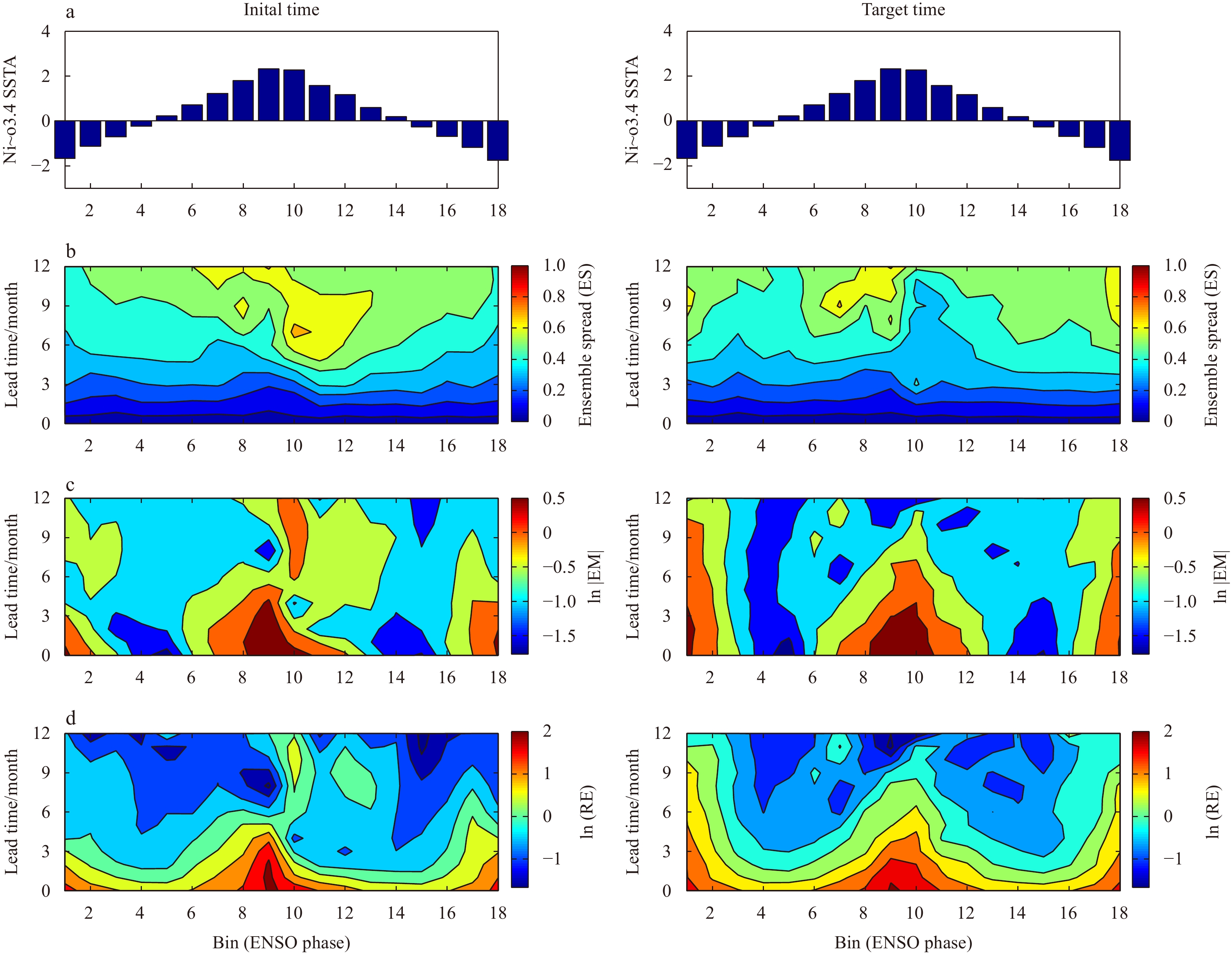
Based on the Ni

Figure 7 reveals large |EM| and RE values to exhibit similar features with the ENSO phase. In particular, large |EM| and RE values occur during the peak ENSO stage, while lower values are linked to the neural phase with weak a ENSO signal. The consistent features between |EM| and RE indicate that RE is dominated by the ENSO signal rather than noise.
In contrast, the ES is less sensitive to the ENSO strength, especially for short lead times. This is true for the strength at both the initial and target times and indicates that the development of the ensemble spread is not related to the ENSO phase in this BCC model. To explore this further, we conducted similar analysis using the ZC model and obtained comparable conclusions (Fig. 8); the |EM| and RE have consistently larger values during the peak ENSO phases, and smaller values during the weak ENSO signal/phases or transition stages. Moreover, the ES does not exhibit larger values in the phase transition stages. These similar features between the BCC and ZC models suggests the “signal-dominate ENSO prediction skills” feature might not be a model-dependent feature.

The ENSO ensemble prediction skill of the BCC-CPS2 model is analyzed using actual and potential prediction skill measures during 1991–2018. Several results related to the ENSO prediction skill of the model are made. First, the RMSE and BSS skill score exhibit a consistent upper-limit of approximately 10 months for ENSO prediction in the BCC-CPS2 model. Second, warm and cold ENSO events have higher prediction skills and a longer predictability than normal ENSO state. The BCC model has 10 months predictability during warm/cold ENSO states but only 6 months predictability during the normal ENSO phase. In addition, the spring barrier with seasonal-dependent performance is a significant character of the model.
The analyses of the ensemble/information-based potential prediction skill metrics indicate the RE (dominated by the ENSO signal component) to surpass the PI and PP in quantifying the correlation-based prediction skill. This is consistent with previous results using simple ENSO models (e.g., the ZC model). Thus, according to this result we can suggest that the information-based potential prediction metric RE is more useful than PP and PI in evaluating an individual ENSO predication skill before the observed SSTA data is issued.
The signal-dependent prediction skill scores suggest that the "spring forecast barrier" of the ENSO prediction is likely to be related to the weak signal phase during boreal spring and early summer. This is consistent with recent ENSO predictability studies (e.g., Kumar and Hu, 2014; Kumar et al., 2017; Hu et al., 2019). An evaluation of the Indian Ocean Dipole (IOD) prediction skill in the BCC model also reveals a similar conclusion (not shown). Our results imply that the signal-dependent feature may present in the predictions of many climate and weather events.
Despite the robustness of our results, caution should be taken. First, compared to the ZC ensemble system, the ensemble forecast of the BCC-CPS model is still far from perfect, with a small ensemble spread ES and large REL scores at the three ENSO states during the forecast period. Without an optimal error growth/perturbation construction scheme, the ensemble spread is not able to grow sufficiently during the forecast period and thus the ensemble mean error RMSE is not sufficiently reduced. The construction of a reliable ensemble system still proves to be a challenging task for complicate climate models. Second, the upper limit predictability of BCC ensemble products is only 10 months, therefore further improvements of BCC model are required. Nevertheless, this work explored the ENSO statistical predictability over the past 29 years using a national level operational seasonal prediction system, which provides insights on the properties of ENSO predictability in an operational prediction system, including its seasonal and phase variation as well the relative contribution of signal and noise to its potential predictability.
Although the initial error growth and ENSO signal intensity are both important factors for ENSO prediction skill. From the current study, we can see ENSO predication skill is dominated by the signal component. The SPB phenomenon can be well explained from this signal-dominant aspect. The initial error growth has limited influence on prediction skill. This conclusion is helpful for model developers, because they can put more work focusing on model system errors rather than the initial error growth.
| [1] |
Cheng Yanjie, Tang Youmin, Chen Dake. 2011. Relationship between predictability and forecast skill of ENSO on various time scales. Journal of Geophysical Research: Oceans, 116(C12): C12006. doi: 10.1029/2011JC007249
|
| [2] |
Cheng Yanjie, Tang Youmin, Jackson P, et al. 2010. Ensemble construction and verification of the probabilistic ENSO prediction in the LDEO5 model. Journal of Climate, 23(20): 5476–5497. doi: 10.1175/2010JCLI3453.1
|
| [3] |
DelSole T. 2004. Predictability and information theory: part I. Measures of predictability. Journal of Atmospheric Sciences, 61(20): 2425–2440. doi: 10.1175/1520-0469(2004)061<2425:PAITPI>2.0.CO;2
|
| [4] |
DelSole T, Tippett M K. 2007. Predictability: Recent insights from information theory. Reviews of Geophysics, 45: RG4002. doi: 10.1029/2006RG000202
|
| [5] |
Griffies S M, Gnanadesikan A, Dixon K W, et al. 2005. Formulation of an ocean model for global climate simulations. Ocean Science, 1: 45–79. doi: 10.5194/os-1-45-2005
|
| [6] |
Hoffman R N, Kalnay E. 1983. Lagged average forecasting, an alternative to Monte Carlo forecasting. Tellus A, 35(2): 100–118. doi: 10.3402/tellusa.v35i2.11425
|
| [7] |
Hu Z Z, Kumar A, Zhu J S, et al. 2019. On the challenge for ENSO cycle prediction: An example from NCEP Climate Forecast System, version 2. Journal of Climate, 32(1): 183–194. doi: 10.1175/JCLI-D-18-0285.1
|
| [8] |
Jin E K, Kinter J L III, Wang B, et al. 2008. Current status of ENSO prediction skill in coupled ocean–atmosphere models. Climate Dynamics, 31(6): 647–664. doi: 10.1007/s00382-008-0397-3
|
| [9] |
Kleeman R. 2002. Measuring dynamical prediction utility using relative entropy. Journal of the Atmospheric Sciences, 59(13): 2057–2072. doi: 10.1175/1520-0469(2002)059<2057:MDPUUR>2.0.CO;2
|
| [10] |
Kleeman R, Tang Y M, Moore A M. 2003. The calculation of climatically relevant singular vectors in the presence of weather noise as applied to the ENSO problem. Journal of the Atmospheric Sciences, 60(23): 2856–2868. doi: 10.1175/1520-0469(2003)060<2856:TCOCRS>2.0.CO;2
|
| [11] |
Kumar A, Hu Z Z. 2014. How variable is the uncertainty in ENSO sea surface temperature prediction?. Journal of Climate, 27(7): 2779–2788. doi: 10.1175/JCLI-D-13-00576.1
|
| [12] |
Kumar A, Hu Z Z, Jha B, et al. 2017. Estimating ENSO predictability based on multi-model hindcasts. Climate Dynamics, 48(1–2): 39–51. doi: 10.1007/s00382-016-3060-4
|
| [13] |
Latif M, Barnett T P, Cane M A, et al. 1994. A review of ENSO prediction studies. Climate Dynamics, 9(4): 167–179
|
| [14] |
McPhaden M J. 2003. Tropical Pacific Ocean heat content variations and ENSO persistence barriers. Geophysical Research Letters, 30(9): 1480. doi: 10.1029/2003GL016872
|
| [15] |
Ren Hongli, Jin F F, Song L C, et al. 2017. Prediction of primary climate variability modes at the Beijing Climate Center. Journal of Meteorological Research, 31(1): 204–223. doi: 10.1007/s13351-017-6097-3
|
| [16] |
Ren Hongli, Scaife A A, Dunstone N, et al. 2019. Seasonal predictability of winter ENSO types in operational dynamical model predictions. Climate Dynamics, 52(7–8): 3869–3890. doi: 10.1007/s00382-018-4366-1
|
| [17] |
Ren Hongli, Zheng Fei, Luo Jingjia, et al. 2020. A review of research on tropical air-sea interaction, ENSO dynamics, and ENSO prediction in China. Journal of Meteorological Research, 34(1): 43–62. doi: 10.1007/s13351-020-9155-1
|
| [18] |
Sohn S J, Tam C Y, Jeong H I. 2016. How do the strength and type of ENSO affect SST predictability in coupled models. Scientific Reports, 6(1): 33790. doi: 10.1038/srep33790
|
| [19] |
Tang Y M, Kleeman R, Moore A M. 2005. Reliability of ENSO dynamical predictions. Journal of the Atmospheric Sciences, 62(6): 1770–1791. doi: 10.1175/JAS3445.1
|
| [20] |
Tang Y M, Kleeman R, Miller S. 2006. ENSO predictability of a fully coupled GCM model using singular vector analysis. Journal of Climate, 19(14): 3361–3377. doi: 10.1175/JCLI3771.1
|
| [21] |
Tang Y M, Lin H, Moore A M. 2008. Measuring the potential predictability of ensemble climate predictions. Journal of Geophysical Research, 113(D4): D04108. doi: 10.1029/2007JD008804
|
| [22] |
Tang Youmin, Zhang Ronghua, Liu Ting, et al. 2018. Progress in ENSO prediction and predictability study. National Science Review, 5(6): 826–839. doi: 10.1093/nsr/nwy105
|
| [23] |
Tian Ben, Ren Hongli, Jin Feifei, et al. 2019. Diagnosing the representation and causes of the ENSO persistence barrier in CMIP5 simulations. Climate Dynamics, 53(3): 2147–2160
|
| [24] |
Wilks D S. 2006. Statistical Methods in the Atmospheric Sciences. 2nd ed. New York: Academic Press, 284–292
|
| [25] |
Winton M. 2000. A reformulated three-layer sea ice model. Journal of Atmospheric and Oceanic Technology, 17(4): 525–531. doi: 10.1175/1520-0426(2000)017<0525:ARTLSI>2.0.CO;2
|
| [26] |
Wu Tongwen, Song Lianchun, Li Weiping, et al. 2014. An overview of BCC climate system model development and application for climate change studies. Journal of Meteorological Research, 28(1): 34–56
|
| [27] |
Wu Tongwen, Yu Rucong, Zhang Fang. 2008. A modified dynamic framework for the atmospheric spectral model and its application. Journal of the Atmospheric Sciences, 65(7): 2235–2253. doi: 10.1175/2007JAS2514.1
|
| [28] |
Zheng Fei, Zhu Jiang. 2010. Spring predictability barrier of ENSO events from the perspective of an ensemble prediction system. Global and Planetary Change, 72(3): 108–117. doi: 10.1016/j.gloplacha.2010.01.021
|
| 1. | Qianqian Qi, Wansuo Duan, Xia Liu, et al. Exploring sensitive area in the whole pacific for two types of El Niño predictions and their implication for targeted observations. Frontiers in Earth Science, 2024, 12 doi:10.3389/feart.2024.1429003 | |
| 2. | Gongjie Wang, Hong-Li Ren, Jingpeng Liu, et al. Seasonal predictions of sea surface height in BCC-CSM1.1m and their modulation by tropical climate dominant modes. Atmospheric Research, 2023, 281: 106466. doi:10.1016/j.atmosres.2022.106466 | |
| 3. | Hong-Li Ren, Qing Bao, Chenguang Zhou, et al. Seamless Prediction in China: A Review. Advances in Atmospheric Sciences, 2023, 40(8): 1501. doi:10.1007/s00376-023-2335-z |

Figures(8)

Supported by:
Beijing Renhe Information Technology Co. Ltd

Yanjie Cheng, Youmin Tang, Tongwen Wu, Xiaoge Xin, Xiangwen Liu, Jianglong Li, Xiaoyun Liang, Qiaoping Li, Junchen Yao, Jinghui Yan. Investigating the ENSO prediction skills of the Beijing Climate Center climate prediction system version 2[J]. Acta Oceanologica Sinica, 2022, 41(5): 99-109. doi: 10.1007/s13131-021-1951-7

 DownLoad:


 DownLoad: