Key Laboratory of Marine Ecosystem Dynamics, Second Institute of Oceanography, Ministry of Natural Resources, Hangzhou 310012, China
2.
School of Marine Sciences, China University of Geosciences, Beijing 100083, China
3.
Southern Marine Science and Engineering Guangdong Laboratory (Zhuhai), Zhuhai 519080, China
Funds:
The National Natural Science Foundation of China under contract No. 42076122; the China Ocean Mineral Resources Research and Development Association Program under contract Nos DY135-E2-3-04, DY135-E2-2-04 and JS-KTFA-2018-01.
The mesopelagic communities are important for food web and carbon pump in ocean, but the large-scale studies of them are still limited until now because of the difficulties on sampling and analyzing of mesopelagic organisms. Mesopelagic organisms, especially micronekton, can form acoustic deep scattering layers (DSLs) and DSLs are widely observed. To explore the spatial patterns of DSLs and their possible influencing factors, the DSLs during daytime (10:00–14:00) were investigated in the subtropical northwestern Pacific Ocean (13°–23.5°N, 153°–163°E) using a shipboard acoustic Doppler current profiler at 38 kHz. The study area was divided into three parts using k-means cluster analysis: the northern part (NP, 22°–24°N), the central part (CP, 17°–22°N), and the southern part (SP, 12°–17°N). The characteristics of DSLs varied widely with latitudinal gradient. Deepest core DSLs (523.5 m±17.4 m), largest nautical area scattering coefficient (NASC) (130.8 m2/n mile2±41.0 m2/n mile2), and most concentrated DSLs (mesopelagic organisms gathering level, 6.7%±0.7%) were observed in NP. The proportion of migration was also stronger in NP (39.7%) than those in other parts (18.6% in CP and 21.5% in SP) for mesopelagic organisms. The latitudinal variation of DSLs was probably caused by changes in oxygen concentration and light intensity of mesopelagic zones. A positive relationship between NASC and primary productivity was identified. A four-months lag was seemed to exist. This study provides the first basin-scale baselines information of mesopelagic communities in the northwest Pacific with acoustic approach. Further researches are suggested to gain understandings of seasonal and annual variations of DSLs in the region.
Deep scattering layers (DSLs) were first discovered using acoustic equipment during World War II. They have been widely explored in the large-scale investigation of nekton communities using acoustic methods featuring rapid sampling, as well as noninvasive and nonextractive advantages (Benoit-Bird and Lawson, 2016). The DSLs are created by micronekton aggregation in the mesopelagic layers. They reflect the behavior of organisms in those layers and are considered to be an important characteristic of the open ocean (Béhagle et al., 2017; Sato and Benoit-Bird, 2017; Boswell et al., 2020).
As one of the largest groups in marine biome, micronekton include small fishes, crustaceans, cephalopods, and gelatinous organisms, with length ranging from 2 cm to 20 cm. Micronekton plays a crucial role in the deep-sea food web (Polis et al., 1997; Klevjer et al., 2020). These organisms migrate to the surface (0–200 m) to feed at night and descend to the mesopelagic layers (200–1 000 m) to escape larger predators after sunrise. This type of behavior is commonly referred to as diel vertical migration. The acoustic signature of micronekton at 38 kHz has been widely used in fishery resource surveys and ecological studies (Bertrand et al., 2002; Moline et al., 2015; Béhagle et al., 2016; Cascão et al., 2019). The biomass of micronekton in the pelagic zone is usually underestimated because of their escape from pelagic trawls. Thus, their role in the oceanic biogeochemical cycle and food web may be much greater than our current understanding (Gjøsaeter and Kawaguchi, 1980; Kloser et al., 2009; FAO, 2018).
The behavior and life history of mesopelagic micronekton are driven by various marine environmental factors that lead to the spatial and temporal features of the DSLs. For instance, the timing and speed of their migration are affected by not only the angle of the sun but also the migration depth and community composition of organisms in the sound scattering layers (Benoit-Bird and Lawson, 2016; Boswell et al., 2020). The environmental properties of water layers, such as dissolved oxygen concentration, temperature, and light intensity, could influence the migration depth of mesopelagic organisms (Bertrand et al., 2010; Aksnes et al., 2017; Diogoul et al., 2020). Primary productivity has been proven to be a key influencing factor of mesopelagic biomass in previous studies (Jennings et al., 2008; Escobar-Flores et al., 2013; Irigoien et al., 2014; Receveur et al., 2020). Scale effects are also frequently found in the responses of horizontal and vertical distributions of DSLs to various environmental variables. For example, at a global or basin scale, the major driving factors of DSLs are sea surface temperature, primary productivity, and dissolved oxygen (Bianchi et al., 2013; Brierley, 2014; Irigoien et al., 2014; Klevjer et al., 2016; Escobar-Flores et al., 2018). Mesoscale oceanographic features (e.g., mesoscale eddies and frontal boundaries) have also been identified as important factors in driving the dynamics of sound scattering layers (Godø et al., 2012; Fennell and Rose, 2015; Béhagle et al., 2016). At a local scale, some oceanographic disturbances (e.g., currents, nutrients, temperature, and dissolved oxygen) caused by seamounts or upwellings, can strengthen the aggregation of organisms and significantly promote the acoustic backscattering strength (Urmy and Horne, 2016; Cascão et al., 2019).
Micronekton is an important part of marine food web in the northwestern Pacific Ocean. Several important commercial fishes (e.g., tunas and billfishes) are largely supported by micronekton in this area (Chikuni, 1985). Moreover, the mesopelagic community including micronekton, was considered to be influenced by global warming and deep-sea mining in the future (Proud et al., 2017; Christiansen et al., 2020). The influences are conspicuous in marine ecological environment due to the complex and unpredictable process of ocean change and the rapidly increasing number of deep-sea mining areas (Mote and Salathé, 2010; Miller et al., 2018). Nevertheless, our understanding of mesopelagic community remains limited (St John et al., 2016). In previous large-scale investigations of DSLs, the spatial distribution of DSLs and their relationships with the marine environment in the subtropical Northwest Pacific Ocean were not well investigated (Irigoien et al., 2014; Bianchi and Mislan, 2016; Klevjer et al., 2016).
To explore the spatial distribution of DSLs and their response to environmental factors, acoustic backscatter data at 38 kHz by shipboard acoustic Doppler current profiler (SADCP) and environmental data obtained during voyage investigation were analyzed. Our research was focused on two objectives. First, the distribution patterns of DSLs were described along the latitudinal gradient. Second, the relationship between DSLs and marine environmental factors was analyzed to evaluate the potential environmental associations of DSLs in the northwestern Pacific Ocean.
Ship-based data collection was conducted with a SADCP, OS38K during COMRA cruise DY48, from August to October 2018. The acoustic transects are shown in Fig. 1. The transducers were mounted on the bottom of ship and with a central frequency of 38 kHz. This frequency allowed the collection of valid data down to a depth of approximately 1 000 m. The sampling interval was 10 min, and the vertical cell interval was 24 m. The measuring range was 50–1 000 m in depth. Although the raw acoustic data were not calibrated or compared with other calibrated equipment, these data are considered suitable for evaluating the relative biomass of mesopelagic community and identifying the vertical distribution of DSLs, according to the principle of acoustic Doppler current profiler (ADCP) (Bianchi and Mislan, 2016; Receveur et al., 2020) (refer to Table 1 for full name, same below).
Figure
1.
Map of the study area (red box in the insert) and the navigation and acoustic recording route (red line). The study area is located in the seamount (brighter colored areas) region of the northwestern Pacific Ocean.
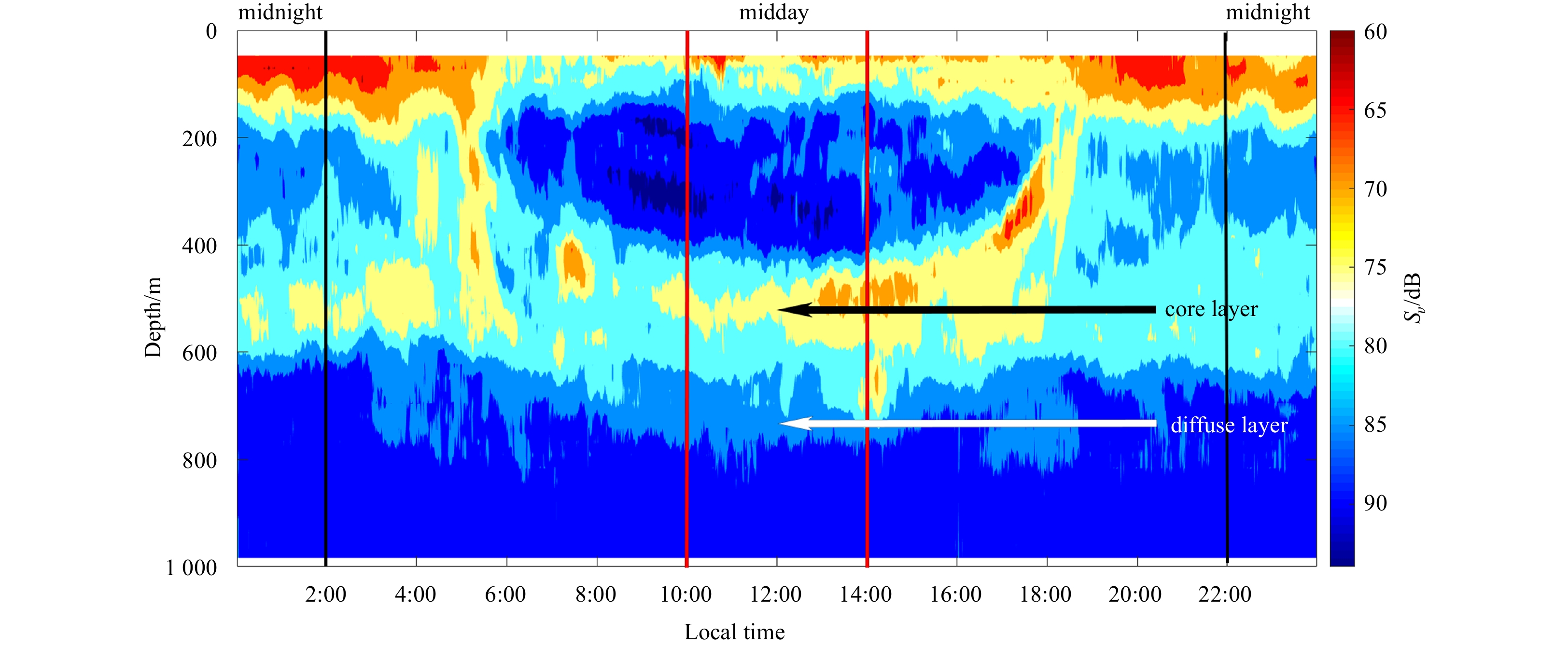
There were continuous DSLs and regular diel vertical migrations along all acoustic transects. In the echogram, the vertical migration of mesopelagic organisms in this area is characterized by descent from the surface at around 6:00, stabilization at a depth of 400–800 m (core region 400–600 m) at around 10:00, and ascent at around 14:00, finally reaching the surface at around 19:00 (Fig. 2).
Figure
2.
Echogram (38 kHz) after noise-removal showing the diel vertical migration of mesopelagic organisms (at local time 0:00–24:00, September 10, 2018). The red lines indicated the period of midday (at local time 10:00–14:00), when the dwelling depth of mesopelagic organisms was relative stable and it was easy to eliminate the disturbance of diel vertical migration. And the black lines indicated the period of midnight (at local time 22:00–next day 2:00). The black arrow indicated the core part of deep scattering layers (DSLs), and the white arrow indicated the diffuse part of DSLs.
Midday and midnight were defined as the periods of 10:00–14:00 and 20:00–02:00, respectively. The acoustic data from midday was mainly used in the subsequent analysis for two reasons. First, a large proportion of mesopelagic organisms migrate up to the surface for feeding, but the 38-kHz SADCP was not appropriate for obtaining data from 0 m to 50 m in depth. In contrast, most of the mesopelagic organisms migrated down to 400–800 m during the day and thus were integrally detected in our investigation. Second, the downwelling depth of mesopelagic organisms was relatively stable, making it easy to eliminate diel vertical migration (DVM) disturbances during these periods (Fig. 2).
The mean volume backscattering strength (MVBS, dB re 4π m−1) was calculated from the recorded backscattering echo intensity E (counts) based on the sonar equation in Mullison (2017),
where Sv means MVBS; C means a system constant provided by the ADCP manufacturer, which includes the transducer and system noise characteristics; C is −172.19 dB for the Workhorse Long Ranger functioning at a frequency of 38 kHz. The other variables are as follows: Tx is the temperature of the transducer (°C); R is the range along the beam to the scatterers (m); LDBM is 10 lg (transmit pulse length, 24 m); PDBM is 24 dB; α is the sound absorption coefficient of seawater (0.011 dB/m); and Kc is a beam-specific scaling factor (dB/count), is typically assumed to be 0.45; Er is the received signal strength indicator (RSSI) value when there is no signal present, which is determined from the minimum values of the RSSI counts obtained from the cell at the most remote depth (Deines, 1999; Mullison, 2017).
Sv is the logarithmic form of sv (volume backscattering coefficient, VBC) in Eq. (2), and sv is integrated with depth using the formula in MacLennan et al. (2002) to produce the area backscattering coefficient, sa (m2/m2). The most common scaled coefficient, the nautical area scattering coefficient (NASC), is denoted by the symbol sA (m2/n mile2) (MacLennan et al., 2002). The NASC calculated from the 38 kHz acoustic frequency was used as a proxy of micronekton biomass (Kloser et al., 2009; Béhagle et al., 2016).
where z means water depth (m) , and sv(z) is the backscattering coefficient at depth z.
The boundaries and central depth of the DSLs were used to describe the vertical distribution of micronekton. The DSL center (CM, m) was derived for the DSL using the approach provided by Urmy et al. (2012) as Eq. (5).
where z1 and z2 represent the upper and lower depths of DSLs’ boundaries.
The threshold filtering method has been used in many studies to identify the location of DSLs. However, these threshold values were not uniform (Béhagle et al., 2016; Klevjer et al., 2016). The DSLs could be divided into two parts, the core DSLs and diffuse DSLs (Fig. 2). The core DSLs represent the main stable blocks of mesopelagic communities. Since the ADCP acoustic data were not calibrated in this study, the threshold method could not be used. Therefore, we used the gradient of backscattering strength as an index of identified DSLs boundaries (Eq. (6)). The values for the gradient (from the surface to deep layer) were used to select the upper boundary and lower boundary. First, the DSLs zone should be estimated from echograms, since the vertical distribution of gradient fluctuated. For example, the DSLs were located at the depths of 400–800 m in the study area (Fig. A1). Second, the maximum and minimum gradient values were selected as points corresponding to the upper and lower boundaries of core DSLs (Fig. 3).
Figure
3.
An example about identifying the boundaries of core deep scattering layers (DSLs) according to gradient method. a. Vertical distribution of mean volume backscattering strength (MVBS); b. vertical distribution of changes in gradient of MVBS. The dots are identified boundaries of core DSLs.
where ∆ is the gradient of backscattering strength (dB/m), and i is the layer number. The DSL thickness was calculated by subtracting the lower DSL depth from the upper DSL depth.
The coefficient of variation (CV) was used to measure the degree of dispersion (Everitt and Skrondal, 1998). In this study, the mesopelagic organisms gathering level (MGL) was explained by the CV of backscatter strength in the mesopelagic zone (Eq. (7)).
where σ is the standard deviation of mesopelagic MVBS (200–1 000 m) and $ \bar{S_v} $ is the mean value of mesopelagic MVBS.
Migration amplitudes (MA) were calculated as the difference between daytime and nighttime mesopelagic NASC (sA (m2/n mile2), 200–1 000 m). The migrating proportion of mesopelagic organisms (MP) was calculated as the ratio of migration amplitudes to mesopelagic daytime NASC values. Weighted migration depth (WMD) was calculated as the weighted mean of the difference between daytime and nighttime mesopelagic NASC and depth in mesopelagic zone (Klevjer et al., 2016).
where sA_day and sA_night are mesopelagic NASC during midday and midnight, respectively. Svday and Svnight are MVBS during midday and midnight, respectively. Finally, i is the layer number of corresponding depth.
2.3
Environmental data collection and processing
A suite of available environmental variables was selected to explore the environmental associations of DSLs. In this study, all environmental data were retrieved from public sources. Monthly average of 490 nm light attenuation coefficient (LAC 490 nm) data with a (1/24)° resolution were obtained from the NASA website (https://search.earthdata.nasa.gov/search?fst0=Oceans). The LAC was calculated as Eq. (11).
where k is LAC and depthx is certain depth underwater. lightx and light0 is the light intensity at the certain depth underwater and surface light intensity, respectively (Padial and Thomaz, 2008).
Monthly average of net primary productivity (NPP) data with a (1/6)° resolution were obtained from the Ocean Productivity website (http://orca.science.oregonstate.edu/1080.by.2160.monthly.hdf.vgpm.m.chl.m.sst.php). Monthly average of mixed layer depth (MLD) data and profile data of temperature and salinity with 1° resolution and 5 m vertical interval were obtained from the Argo website (http://mixedlayer.ucsd.edu/). Monthly average of oceanic dissolved oxygen concentration profile data with a 1° resolution comes from the world oceanic database (WOD, https://www.ncei.noaa.gov/access/world-ocean-atlas-2018/). Three environmental variables mesopelagic average temperature, salinity, and dissolved oxygen concentration (mesopelagic average temperature (MAT), mesopelagic averagesalinity (MAS), and mesopelagic average dissolved oxygen (MAO)) at 200–1 000 m were also calculated to describe the mesopelagic zone. The natural adjacent interpolation method (Sibson, 1981) was used to process the gridded environmental data and match it with each acoustic location, thereby obtaining profile data for each point.
2.4
Statistical analysis
A k-means cluster analysis (Legendre and Legendre, 2012) of environmental variables (MLD, sea surface temperature (SST), sea surface salinity (SSS), MAT, MAS, MAO, LAC, and NPP) was used to divide the study area into different environmental groups. The distributions normality and variance homogeneity of the data were tested first. If the hypothesis was not met, non-parametric tests (Kruskal-Wallis test) were used to test the difference among groups.
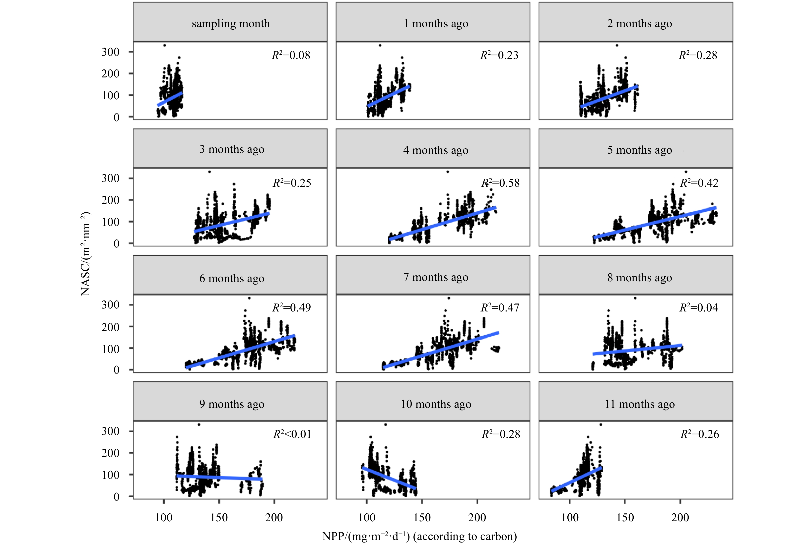
To reveal the relationships between primary productivity during different months and NASC, we used remote-sensing data to construct a new dataset of monthly NPP for the 12 months before the cruise period (August–October) according to the month of each station. Twelve linear regression analyses were conducted to detect the time lag in the link between NPP and NASC. The statistical analysis for this part was performed using R-3.6.3. The linear regressions were conducted using the lme function of the mgcv R package (Lindstrom and Bates, 1988).
3.
Results
3.1
Environmental conditions
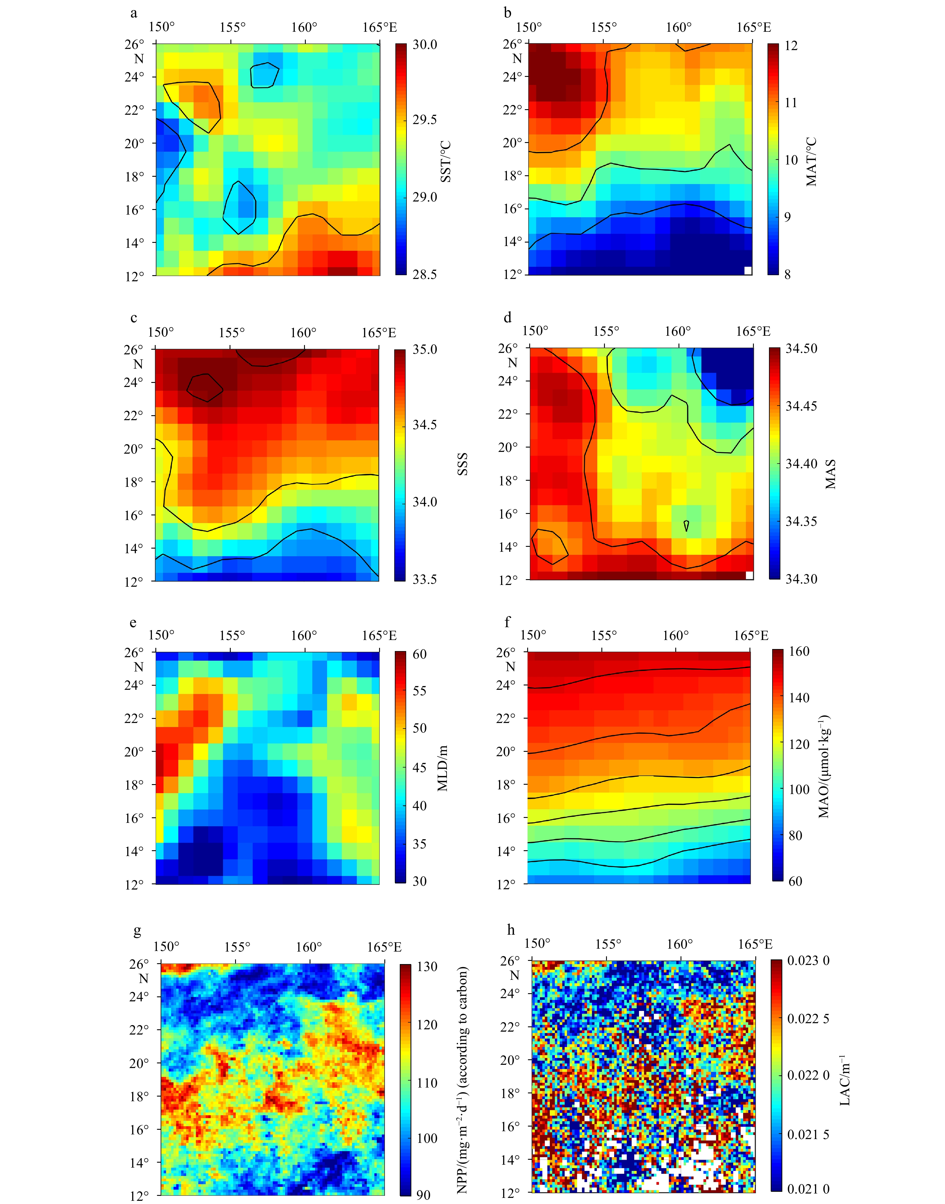
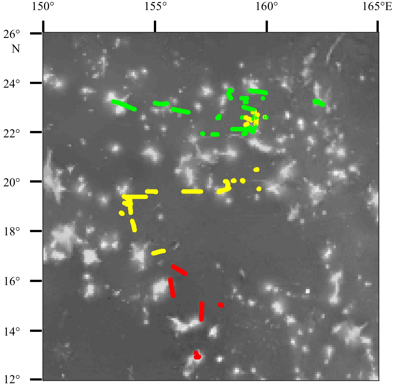
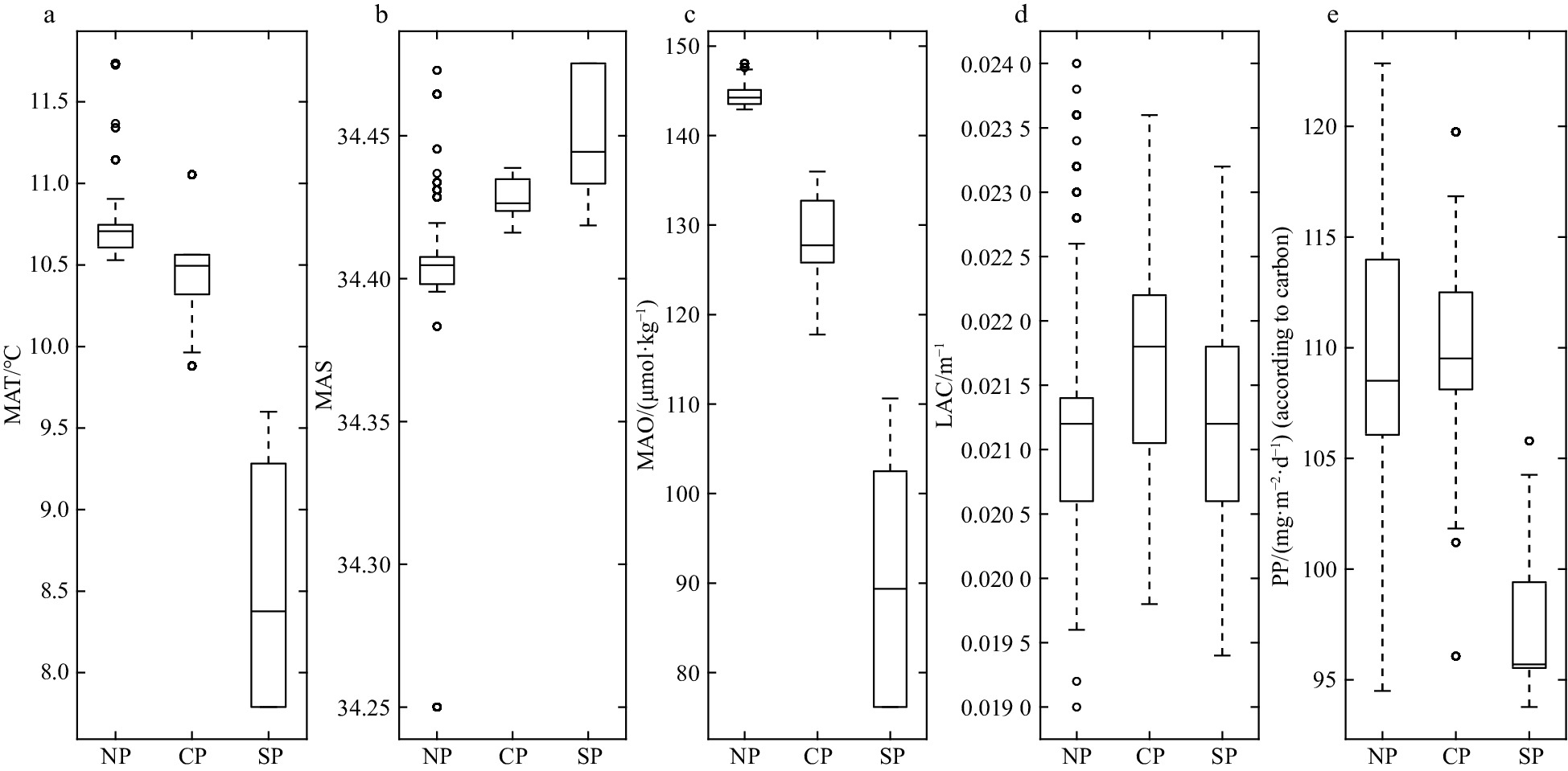
Strong latitudinal gradients of environmental variables were observed in this area. (Fig. 4). Based on the results of cluster analysis, three environmental parts were identified: the northern part (NP, 22°–24°N), the central part (CP, 17°–22°N), and the southern part (SP, 12°–17°N) (Fig. 5). The SP was distinguished from other parts by the lowest values of MAT (8.5°C±0.7°C) and MAO (89.9 μmol/kg±13.0 μmol/kg). In contrast, the mesopelagic community of NP was located in warmer (MAT, 10.7°C±0.2°C), and oxygen-rich (144.4 μmol/kg±1.2 μmol/kg) conditions (Fig. 6).
Figure
4.
Maps of environmental conditions in the study area (the average data during September was used for mapping). a, b. Sea surface temperature (SST) and mesopelagic average temperature (MAT); c, d. sea surface salinity (SSS) and mesopelagic average salinity (MAS); e. mixing layer depth (MLD); f. mesopelagic average dissolved oxygen concentration (MAO); g. net primary productivity (NPP); h. 490 nm light attenuation coefficient (LAC). The black curves in some images are isolines.
Figure
5.
The distribution of environmental variables according to k-means clustering methods in study area. Green group is the northern part, yellow group is the central part, and red group is the southern part.
Figure
6.
Box plots about the features of environment in three parts (NP, northern part; CP, central part; SP, southern part). a. Mesopelagic average temperature (MAT); b. mesopelagic average salinity (MAS); c. mesopelagic average dissolved oxygen concentration (MAO); d. 490 nm light attenuation coefficient (LAC); e. primary productivity (PP).
The distribution of DSLs also showed a strong latitudinal gradient. The spatial variation of DSLs among three parts was significant (Kruskal-Wails test, p<0.01). The mesopelagic NASC of NP ((130.8±41.0) m2/n mile2) was 2.4 times higher than that of CP ((55.2±27.3) m2/n mile2), and 5.9 times higher than that of SP ((22.2±5.5) m2/n mile2) (Fig. 7a). A shallower CM ((502.1±21.8) m) was observed in SP than those in NP ((532.5±17.4) m) and CP ((524.0±17.0) m) (Fig. 7b). The gathering level showed that the mesopelagic organisms were more diffuse in SP (3.3%±0.5%) than those in NP (6.7%±0.7%) and CP (5.6%±0.8%) (Fig. 7c). Both the upper boundary depth (UBD) and lower boundary depth (LBD) showed a shallower trend along the latitudinal gradient from the north to the south (Figs 7d, e).
Figure
7.
Box plots about the features of deep scattering layers (DSLs), showing the differences among three parts (NP, northern part; CP, central part; SP, southern part). a. Mesopelagic nautical area scattering coefficient (MNASC); b. center mass (CM); and c. mesopelagic gathering level (MGL) of mesopelagic zone. d and e showed the upper (UBD) and lower boundary depth (LBD) of DSLs, respectively.
The characteristics of DVM of mesopelagic organism also showed strong spatial variation (Fig. 8). The MP in NP, CP, and SP were 39.7%, 18.6%, and 21.5%, respectively. The average WMD gradually increase along the latitudinal gradient from the north to the south (574 m, 606 m, 663 m, in NP, CP, and SP, respectively).
Figure
8.
Vertical distribution of acoustic backscatter grouped into three parts, according to the result of k-means cluster analysis. a, northern part; b, central part; c, southern part. Red lines show average midday-time profiles (10:00–14:00), and light red shadows are range of standard deviations. Black lines show average midnight-time profiles (22:00–next day 2:00), and gray shadows are range of standard deviations. x-axis is acoustic backscatter measured as nautical area scattering coefficient (NASC) at the corresponding depth.
3.4
Relationships between mesopelagic NASC and primary production
We attempted to detect whether there were any possible delays in the transfer of primary production to the upper trophic levels. The variances of correlations between NASC values during the cruise period and NPP values in the previous 12 months were distinct (Fig. A2). During the sampling time, the linear correlation coefficient between the mesopelagic NASC and NPP was weak (R2=0.08, p<0.05). With an increasing time lag, the link between NASC and NPP became stronger and peaked at four months leg (R2=0.58). The NASC was significantly positively correlated with NPP at lags of 4–7 months (R2, 0.42–0.58), while the link was weak in other months (Fig. A1).
4.
Discussion
4.1
Spatial variation of DSLs
The dissolved oxygen of water column has been proposed as a key factor affecting the depth of DVM (Bianchi et al., 2013; Netburn and Anthony Koslow, 2015; Klevjer et al., 2016). There are two possible reasons. First, the oxygen could affect the metabolism and behavior of organism and communities (Seibel, 2011). However, some species of micronekton have strong adaptation to low oxygen conditions, the depth of DSLs would be affected, only in some extreme hypoxia zones (Urmy et al., 2012; Netburn and Anthony Koslow, 2015). Second, to avoid the predators with higher oxygen demand (e.g., billfishes, tropical tunas, and other tropical pelagic fishes), mesopelagic organisms descend to the layers with low oxygen levels for refuge during the daytime (Stramma et al., 2012).
In the study area, stronger stratification at lower latitudes resulted in a lower mesopelagic average oxygen concentration in SP than that in NP. The average oxygen concentration of mesopelagic layers in the study area is unlikely to limit the vertical distribution of DSLs directly, since the oxygen levels are far from extremely hypoxic (<23 μmol/kg; Netburn and Anthony Koslow, 2015).
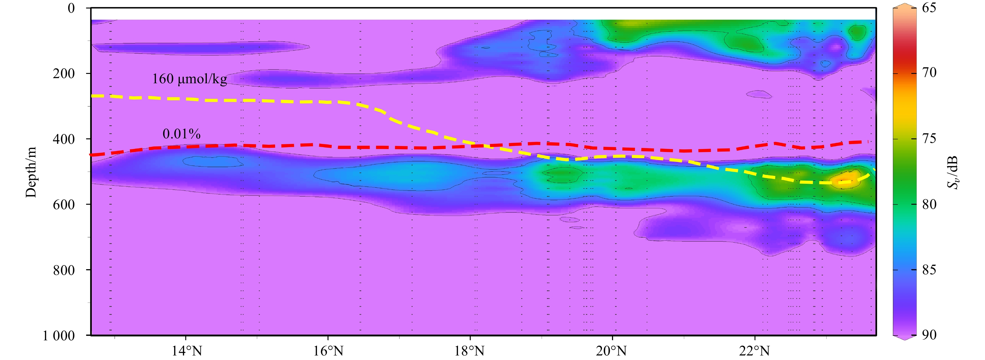
Skipjack and tuna were the main predators of micronekton (Coull, 1993). They were more sensitive to oxygen concentration (>160 μmol/kg), compared with mesopelagic organisms (Cayre, 1991; Ingham et al., 1977; Prince and Goodyear, 2006). The limitation of <160 μmol/kg oxygen concentration on these predators would influence the vertical distribution of DSLs. Another factor potentially affecting the depth of DSLs is light intensity, which can limit above predators relying on sight (Bianchi and Mislan, 2016; Inoue et al., 2016; Aksnes et al., 2017; Boswell et al., 2020). Colored dissolved organic matter is an important light absorber in the water column, and it is mainly produced by phytoplankton (Stedmon and Nelson, 2015; Oestreich et al., 2016). In the study area, the DSLs were persistently deeper than the depth of 0.01% surface light intensity (Fig. 9), which was figured as an imporant impact factor for DSL (Aksnes et al., 2017). We concluded that the light intensity controlled the vertical distribution of DSLs on the whole; nevertheless, the distribution pattern of CM depths (deeper in the north and shallower in the south, Fig. 7b) was influenced by the restriction of dissolved oxygen on the predator in mesopelagic zones.
Figure
9.
The echogram at midday along latitudinal gradient. The yellow curve is 160 μmol/kg dissolved oxygen isoline and the red curve is the depth of 0.01% surface light intensity isoline.
This active carbon flux has been widely considered to be an important carbon resource for bathypelagic and seafloor communities in the deep sea (Steinberg et al., 2008b; Grabowski et al., 2019; Hernández-León et al., 2020). The migrating proportion and weighted migration depth are two key parameters to evaluate the DVM of mesopelagic community. The carbon export of biological pump is dependent on many factors: the migrating biomass, the metabolism rate and the depth of migration (Longhurst and Glen Harrison, 1989; Steinberg et al., 2008a; Kwong et al., 2020). Therefore, the spatial variation of DVM can provide an important biological oceanographic reference for the establishment of regional environmental management plans by the International Seabed Authority.
The mesopelagic fishes can be divided into two groups: migrating and non-migrating by their behavior, and the migrating fishes have higher metabolism rate than non-migrating fishes (Salvanes and Kristoffersen, 2001). It indicates that the biological carbon pump of micronekton was highest in the NP because of the highest migrating proportion and amplitude among the three parts. It can be predicted that the carbon pump of micronekton will weaken by the global warming due to the hypoxia expansion and decline of primary productivity (Keeling et al., 2010; Steinacher et al., 2010). However, more precise evaluation of this active flux could not be achieved in this study due to the lack of appropriate samples for calculating the biomass and metabolic rate of mesopelagic species (Ariza et al., 2015; Pakhomov et al., 2019). In future studies, a combination of acoustic survey and trawl sampling is needed.
4.3
The link between NASC and primary production
The main taxa of mesopelagic micronekton in tropical and subtropical oceans are Myctophidae and Cyclothone (Gorelova, 1984; Phillips et al., 2009; Escobar-Flores et al., 2013). They have a short life span and low fecundity rates (McKelvie , 1989; Catul et al., 2011). A recent study showed that a linear correlation between Sv-ADCP (75 kHz) and Sv-EK60 (70 kHz) was significant (Receveur et al., 2020). It indicated the uncalibrated ADCP acoustic data is suitable for evaluating their relative biomass.
The subtropical Pacific Ocean is a typical oligotrophic ecosystem where the primary productivity is strongly limited by nutrient concentrations (Karl et al., 2001; Shen and Shi, 2002). In low-productivity areas, bottom-up control dominates the marine food web, and primary productivity is thus a key factor that controls the biomass of higher trophic levels (Jennings et al., 2008). The primary productivity is dominated by picoplankton in the tropical oligotrophic ocean (Liu et al., 1997). This means that the trophic web is dominated by microbial loops and the time of energy transfer from primary producer to higher trophic organisms is extended. Moreover, the mesopelagic fishes generally own short lifespans in low latitudes, and most of mesopelagic species spawn only once in their lifetime (Salvanes and Kristoffersen, 2001). The 38 kHz acoustics have an object detection limit of 2 cm and larger (McKelvie, 1989; Catul et al., 2011), thereby mesopelagic fishes were only detectable when they grow up from tiny eggs, which must take a time period. Therefore, the ontogenesis of mesopelagic organisms and the limited target size of acoustic detection method both could result in the time lag between our observed peaks of NASC and the primary productivity.
The time lag between primary production and higher trophic levels was also observed in other studies. For example, Urmy and Horne (2016) reported that the response time of increase of zooplankton and micronekton biomass to surface high productivity burst gradually extended from surface to deep layers, based on their time series observation data in the Monterey Bay. Other studies revealed that there were five months delay of biomass of micronekton following the chlorophyll a peak during July–August period (Condie and Dunn, 2006; Smeti et al., 2015). Moreover, primary productivity reached its peak during the spring in the north of study area (Fig. A3), which was consistent with the seasonal variation of primary productivity in the North Pacific Subtropical Gyre (Longhurst, 2007). In addition, the southern part of study area exhibited low primary productivity conditions all year round (Fig. A3). The regional differences reflected obvious seasonal variations in the horizontal distribution of primary productivity along the latitudinal gradient and accounted for the delay effect observed in our study.
Acknowledgements
We thank three reviewers and the editor for their valuable advices in preparing the manuscript. We thank the members of R/V Da Yang Yi Hao for their help during the investigation. We would also thank LetPub (www.letpub.com) for its linguistic assistance.
A1.
Midday vertical distributions of backscattering strength and its changing gradient in the whole study area. a, b. The vertical distributions of increasing gradient and decreasing gradient, respectively; c. the vertical distribution of mean volume backscattering strength (MVBS). Black curves are identified upper and lower boundaries of DSLs (UBD and LBD). x-axis is the column data number.
A2.
The linear correlations between the mesopelagic nautical area scattering coefficient (NASC) during cruise and net primary productivity (NPP) in the past twelve months. The blue lines were fitting curves with R2(p<0.05).
Aksnes D L, Røstad A, Kaartvedt S, et al. 2017. Light penetration structures the deep acoustic scattering layers in the global ocean. Science Advances, 3(5): e1602468. doi: 10.1126/sciadv.1602468
[2]
Ariza A, Garijo J C, Landeira J M, et al. 2015. Migrant biomass and respiratory carbon flux by zooplankton and micronekton in the subtropical Northeast Atlantic Ocean (Canary Islands). Progress in Oceanography, 134: 330–342. doi: 10.1016/j.pocean.2015.03.003
[3]
Béhagle N, Cotté C, Lebourges-Dhaussy A, et al. 2017. Acoustic distribution of discriminated micronektonic organisms from a bi-frequency processing: the case study of eastern Kerguelen oceanic waters. Progress in Oceanography, 156: 276–289. doi: 10.1016/j.pocean.2017.06.004
[4]
Béhagle N, Cotté C, Ryan T E, et al. 2016. Acoustic micronektonic distribution is structured by macroscale oceanographic processes across 20–50°S latitudes in the South-Western Indian Ocean. Deep-Sea Research Part I: Oceanographic Research Papers, 110: 20–32. doi: 10.1016/j.dsr.2015.12.007
[5]
Benoit-Bird K J, Lawson G L. 2016. Ecological insights from pelagic habitats acquired using active acoustic techniques. Annual Review of Marine Science, 8(1): 463–490. doi: 10.1146/annurev-marine-122414-034001
[6]
Bertrand A, Ballón M, Chaigneau A. 2010. Acoustic observation of living organisms reveals the upper limit of the oxygen minimum zone. PLoS ONE, 5(4): e10330. doi: 10.1371/journal.pone.0010330
[7]
Bertrand A, Bard F X, Josse E. 2002. Tuna food habits related to the micronekton distribution in French Polynesia. Marine Biology, 140(5): 1023–1037. doi: 10.1007/s00227-001-0776-3
[8]
Bianchi D, Galbraith E D, Carozza D A, et al. 2013. Intensification of open-ocean oxygen depletion by vertically migrating animals. Nature Geoscience, 6(7): 545–548. doi: 10.1038/ngeo1837
[9]
Bianchi D, Mislan K A S. 2016. Global patterns of diel vertical migration times and velocities from acoustic data. Limnology and Oceanography, 61(1): 353–364. doi: 10.1002/lno.10219
[10]
Boswell K M, D’Elia M, Johnston M W, et al. 2020. Oceanographic structure and light levels drive patterns of sound scattering layers in a low-latitude oceanic system. Frontiers in Marine Science, 7: 51. doi: 10.3389/fmars.2020.00051
[11]
Brierley A S. 2014. Diel vertical migration. Current Biology, 24(22): R1074–R1076. doi: 10.1016/j.cub.2014.08.054
[12]
Carr M E, Friedrichs M A M, Schmeltz M, et al. 2006. A comparison of global estimates of marine primary production from ocean color. Deep-Sea Research Part II: Topical Studies in Oceanography, 53(5−7): 741–770. doi: 10.1016/j.dsr2.2006.01.028
[13]
Cascão I, Domokos R, Lammers M O, et al. 2019. Seamount effects on the diel vertical migration and spatial structure of micronekton. Progress in Oceanography, 175: 1–13. doi: 10.1016/j.pocean.2019.03.008
[14]
Catul V, Gauns M, Karuppasamy P K. 2011. A review on mesopelagic fishes belonging to family Myctophidae. Reviews in Fish Biology and Fisheries, 21(3): 339–354. doi: 10.1007/s11160-010-9176-4
[15]
Cayre P. 1991. Behaviour of yellowfin tuna (Thunnus albacares) and skipjack tuna (Katsuwonus pelarnis) around fish aggregating devices (FADs) in the Comoros Islands as determined by ultrasonic tagging. Aquatic Living Resources, 4(1): 1–12. doi: 10.1051/alr/1991000
[16]
Chikuni S. 1985. The fish resources of the Northwest Pacific. Rome: FAO
[17]
Christiansen B, Denda A, Christiansen S. 2020. Potential effects of deep seabed mining on pelagic and benthopelagic biota. Marine Policy, 114: 103442. doi: 10.1016/j.marpol.2019.02.014
[18]
Condie S A, Dunn J R. 2006. Seasonal characteristics of the surface mixed layer in the Australasian region: implications for primary production regimes and biogeography. Marine and Freshwater Research, 57(6): 569–590. doi: 10.1071/MF06009
[19]
Coull J R. 1993. World Fisheries Resources. New York: Routledge, 6–18
[20]
Deines K L. 1999. Backscatter estimation using broadband acoustic Doppler current profilers. In: Proceedings of the IEEE Sixth Working Conference on Current Measurement. San Diego, CA: IEEE, 249–253
[21]
Diogoul N, Brehmer P, Perrot Y, et al. 2020. Fine-scale vertical structure of sound-scattering layers over an east border upwelling system and its relationship to pelagic habitat characteristics. Ocean Science, 16(1): 65–81. doi: 10.5194/os-16-65-2020
[22]
Escobar-Flores P, O’Driscoll R L, Montgomery J C. 2013. Acoustic characterization of pelagic fish distribution across the South Pacific Ocean. Marine Ecology Progress Series, 490: 169–183. doi: 10.3354/meps10435
[23]
Escobar-Flores P, O’Driscoll R L, Montgomery J C. 2018. Spatial and temporal distribution patterns of acoustic backscatter in the New Zealand sector of the Southern Ocean. Marine Ecology Progress Series, 592: 19–35. doi: 10.3354/meps12489
[24]
Everitt B S, Skrondal A. 1998. The Cambridge Dictionary of Statistics. Cambridge: Cambridge University Press, 89
[25]
FAO. 2018. The state of world fisheries and aquaculture. Rome: FAO
[26]
Fennell S, Rose G. 2015. Oceanographic influences on Deep Scattering Layers across the North Atlantic. Deep-Sea Research Part I: Oceanographic Research Papers, 105: 132–141. doi: 10.1016/j.dsr.2015.09.002
[27]
Gjøsaeter J, Kawaguchi K. 1980. A review of the world resources of mesopelagic fish. Rome: FAO
[28]
Godø O R, Samuelsen A, Macaulay G J, et al. 2012. Mesoscale eddies are oases for higher trophic marine life. PLoS ONE, 7(1): e30161. doi: 10.1371/journal.pone.0030161
[29]
Gorelova T A. 1984. A quantitative assessment of consumption of zooplankton by epipelagic lanternfishes (family Myctophidae) in the equatorial Pacific Ocean. Journal of Ichthyology, 23: 106–113
[30]
Grabowski E, Letelier R M, Laws E A, et al. 2019. Coupling carbon and energy fluxes in the North Pacific Subtropical Gyre. Nature Communications, 10: 1895. doi: 10.1038/s41467-019-09772-z
[31]
Hernández-León S, Koppelmann R, Fraile-Nuez E, et al. 2020. Large deep-sea zooplankton biomass mirrors primary production in the global ocean. Nature Communications, 11(1): 6048. doi: 10.1038/s41467-020-19875-7
[32]
Hu Dunxin, Wu Lixin, Cai Wenju, et al. 2015. Pacific western boundary currents and their roles in climate. Nature, 522(7556): 299–308. doi: 10.1038/nature14504
[33]
Ingham M C, Cook S K, Hausknecht K A. 1977. Oxycline characteristics and skipjack tuna distribution in the southeastern tropical Atlantic. Fishery Bulletin, 75(4): 857–865
[34]
Inoue R, Kitamura M, Fujiki T. 2016. Diel vertical migration of zooplankton at the S1 biogeochemical mooring revealed from acoustic backscattering strength. Journal of Geophysical Research:Oceans, 121(2): 1031–1050. doi: 10.1002/2015JC011352
[35]
Irigoien X, Klevjer T A, Røstad A, et al. 2014. Large mesopelagic fishes biomass and trophic efficiency in the open ocean. Nature Communications, 5: 3271. doi: 10.1038/ncomms4271
[36]
Jennings S, Mélin F, Blanchard J L, et al. 2008. Global-scale predictions of community and ecosystem properties from simple ecological theory. Proceedings of the Royal Society B: Biological Sciences, 275(1641): 1375–1383. doi: 10.1098/rspb.2008.0192
[37]
Karl D M, Bidigare R R, Letelier R M. 2001. Long-term changes in plankton community structure and productivity in the North Pacific Subtropical Gyre: The domain shift hypothesis. Deep-Sea Research Part II: Topical Studies in Oceanography, 48(8−9): 1449–1470. doi: 10.1016/S0967-0645(00)00149-1
[38]
Keeling R F, Körtzinger A, Gruber N. 2010. Ocean deoxygenation in a warming world. Annual Review of Marine Science, 2: 199–229. doi: 10.1146/annurev.marine.010908.163855
[39]
Klevjer T A, Irigoien X, Røstad A, et al. 2016. Large scale patterns in vertical distribution and behaviour of mesopelagic scattering layers. Scientific Reports, 6: 19873. doi: 10.1038/srep19873
[40]
Klevjer T, Melle W, Knutsen T, et al. 2020. Micronekton biomass distribution, improved estimates across four north Atlantic basins. Deep-Sea Research Part II: Topical Studies in Oceanography, 180: 104691. doi: 10.1016/j.dsr2.2019.104691
[41]
Kloser R J, Ryan T E, Young J W, et al. 2009. Acoustic observations of micronekton fish on the scale of an ocean basin: potential and challenges. ICES Journal of Marine Science, 66(6): 998–1006. doi: 10.1093/icesjms/fsp077
[42]
Kwong L E, Henschke N, Pakhomov E A, et al. 2020. Mesozooplankton and micronekton active carbon transport in contrasting eddies. Frontiers in Marine Science, 6: 825. doi: 10.3389/fmars.2019.00825
Lindstrom M J, Bates D M. 1988. Newton-raphson and EM algorithms for linear mixed-effects models for repeated-measures data. Journal of the American Statistical Association, 83(404): 1014–1022
[45]
Lindstrom E, Lukas R, Fine R, et al. 1987. The western equatorial Pacific Ocean circulation study. Nature, 330(6148): 533–537. doi: 10.1038/330533a0
[46]
Liu H, Nolla H A, Campbell L. 1997. Prochlorococcus growth rate and contribution to primary production in the equatorial and subtropical North Pacific Ocean. Aquatic Microbial Ecology, 12(1): 39–47
[47]
Longhurst A R. 2007. Ecological Geography of the Sea. 2nd ed. London: Academic Press, 327–385
[48]
Longhurst A R, Glen Harrison W. 1989. The biological pump: profiles of plankton production and consumption in the upper ocean. Progress in Oceanography, 22(1): 47–123. doi: 10.1016/0079-6611(89)90010-4
[49]
MacLennan D N, Fernandes P G, Dalen J. 2002. A consistent approach to definitions and symbols in fisheries acoustics. ICES Journal of Marine Science, 59(2): 365–369. doi: 10.1006/jmsc.2001.1158
[50]
McKelvie D S. 1989. Latitudinal variation in aspects of the biology of Cyclothone braueri and C. microdon (Pisces: Gonostomatidae) in the eastern North Atlantic Ocean. Marine Biology, 102(3): 413–424. doi: 10.1007/BF00428494
[51]
Miller K A, Thompson K F, Johnston P, et al. 2018. An overview of seabed mining including the current state of development, environmental impacts, and knowledge gaps. Frontiers in Marine Science, 4: 418. doi: 10.3389/fmars.2017.00418
[52]
Moline M A, Benoit-Bird K, O’Gorman D, et al. 2015. Integration of scientific echo sounders with an adaptable autonomous vehicle to extend our understanding of animals from the surface to the bathypelagic. Journal of Atmospheric and Oceanic Technology, 32(11): 2173–2186. doi: 10.1175/JTECH-D-15-0035.1
[53]
Mote P W, Salathé E P. 2010. Future climate in the Pacific Northwest. Climatic Change, 102(1−2): 29–50. doi: 10.1007/s10584-010-9848-z
[54]
Mullison J. 2017. Backscatter estimation using broadband acoustic Doppler current profilers-updated. In: Hydraulic Measurements & Experimental Methods Conference. Durham, NH: ASCE
[55]
Netburn A N, Anthony Koslow J. 2015. Dissolved oxygen as a constraint on daytime deep scattering layer depth in the southern California current ecosystem. Deep-Sea Research Part I: Oceanographic Research Papers, 104: 149–158. doi: 10.1016/j.dsr.2015.06.006
[56]
Oestreich W K, Ganju N K, Pohlman J W, et al. 2016. Colored dissolved organic matter in shallow estuaries: relationships between carbon sources and light attenuation. Biogeosciences, 13(2): 583–595. doi: 10.5194/bg-13-583-2016
[57]
Padial A A, Thomaz S M. 2008. Prediction of the light attenuation coefficient through the Secchi disk depth: empirical modeling in two large Neotropical ecosystems. Limnology, 9(2): 143–151. doi: 10.1007/s10201-008-0246-4
[58]
Pakhomov E A, Podeswa Y, Hunt B P V, et al. 2019. Vertical distribution and active carbon transport by pelagic decapods in the North Pacific Subtropical Gyre. ICES Journal of Marine Science, 76(3): 702–717. doi: 10.1093/icesjms/fsy134
[59]
Phillips A J, Brodeur R D, Suntsov A V. 2009. Micronekton community structure in the epipelagic zone of the northern California Current upwelling system. Progress in Oceanography, 80(1−2): 74–92. doi: 10.1016/j.pocean.2008.12.001
[60]
Polis G A, Anderson W B, Holt R D. 1997. Toward an integration of landscape and food web ecology: the dynamics of spatially subsidized food webs. Annual Review of Ecology and Systematics, 28(1): 289–316. doi: 10.1146/annurev.ecolsys.28.1.289
[61]
Prince E D, Goodyear C P. 2006. Hypoxia-based habitat compression of tropical pelagic fishes. Fisheries Oceanography, 15(6): 451–464. doi: 10.1111/j.1365-2419.2005.00393.x
[62]
Proud R, Cox M J, Brierley A S. 2017. Biogeography of the global ocean’s mesopelagic zone. Current Biology, 27(1): 113–119. doi: 10.1016/j.cub.2016.11.003
[63]
Receveur A, Kestenare E, Allain V, et al. 2020. Micronekton distribution in the Southwest Pacific (New Caledonia) inferred from shipboard-ADCP backscatter data. Deep-Sea Research Part I: Oceanographic Research Papers, 159: 103237. doi: 10.1016/j.dsr.2020.103237
[64]
Salvanes A G V, Kristoffersen J B. 2001. Mesopelagic fishes. In: Steel J, Thorpe S, Turekian K, eds. Encyclopedia of Ocean Sciences. San Diego: Academic Press, 1711–1717
[65]
Sato M, Benoit-Bird K J. 2017. Spatial variability of deep scattering layers shapes the Bahamian mesopelagic ecosystem. Marine Ecology Progress Series, 580: 69–82. doi: 10.3354/meps12295
[66]
Seibel B A. 2011. Critical oxygen levels and metabolic suppression in oceanic oxygen minimum zones. Journal of Experimental Biology, 214(2): 326–336. doi: 10.1242/jeb.049171
[67]
Shen G, Shi B. 2002. Primary Production in Marine. Beijing: Science Press, 189–223
[68]
Sibson R. 1981. A brief description of natural neighbor interpolation. In: Barnett V, ed. Interpreting Multivariate Data. New York: John Wiley & Sons, 21–36
[69]
Smeti H, Pagano M, Menkes C, et al. 2015. Spatial and temporal variability of zooplankton off New Caledonia (Southwestern Pacific) from acoustics and net measurements. Journal of Geophysical Research: Oceans, 120(4): 2676–2700. doi: 10.1002/2014JC010441
[70]
St John M A, Borja A, Chust G, et al. 2016. A dark hole in our understanding of marine ecosystems and their services: Perspectives from the mesopelagic community. Frontiers in Marine Science, 3: 31
[71]
Stedmon C A, Nelson N B. 2015. The optical properties of DOM in the ocean. In: Hansell D A, Carlson C A, eds. Biogeochemistry of Marine Dissolved Organic Matter. 2nd ed. San Diego: Academic Press, 481–508
[72]
Steinacher M, Joos F, Frölicher T L, et al. 2010. Projected 21st century decrease in marine productivity: a multi-model analysis. Biogeosciences, 7(3): 979–1005. doi: 10.5194/bg-7-979-2010
[73]
Steinberg D K, Cope J S, Wilson S E, et al. 2008a. A comparison of mesopelagic mesozooplankton community structure in the subtropical and subarctic North Pacific Ocean. Deep-Sea Research Part II: Topical Studies in Oceanography, 55(14−15): 1615–1635. doi: 10.1016/j.dsr2.2008.04.025
[74]
Steinberg D K, Van Mooy B A S, Buesseler K O, et al. 2008b. Bacterial vs. zooplankton control of sinking particle flux in the ocean’s twilight zone. Limnology and Oceanography, 53(4): 1327–1338. doi: 10.4319/lo.2008.53.4.1327
[75]
Stramma L, Prince E D, Schmidtko S, et al. 2012. Expansion of oxygen minimum zones may reduce available habitat for tropical pelagic fishes. Nature Climate Change, 2(1): 33–37. doi: 10.1038/nclimate1304
[76]
Toole J M, Zou E, Millard R C. 1988. On the circulation of the upper waters in the western equatorial Pacific Ocean. Deep-Sea Research Part A. Oceanographic Research Papers, 35(9): 1451–1482
[77]
Urmy S S, Horne J K. 2016. Multi-scale responses of scattering layers to environmental variability in Monterey Bay, California. Deep-Sea Research Part I: Oceanographic Research Papers, 113: 22–32. doi: 10.1016/j.dsr.2016.04.004
[78]
Urmy S S, Horne J K, Barbee D H. 2012. Measuring the vertical distributional variability of pelagic fauna in Monterey Bay. ICES Journal of Marine Science, 69(2): 184–196. doi: 10.1093/icesjms/fsr205
[79]
Zhang Dongsheng, Wang Chunsheng, Liu Zhensheng, et al. 2012. Spatial and temporal variability and size fractionation of chlorophyll a in the tropical and subtropical Pacific Ocean. Acta Oceanologica Sinica, 31(3): 120–131. doi: 10.1007/s13131-012-0212-1
Ting Chen, Shuai Zhang, Peiwen Jiang, et al. Detecting fish community structure in open waters using environmental DNA: a case study from the central South China Sea. Frontiers in Marine Science, 2025, 12 doi:10.3389/fmars.2025.1544827
2.
Marian Peña. Atlantic versus Mediterranean deep scattering layers around the Iberian peninsula. Progress in Oceanography, 2024, 221: 103211. doi:10.1016/j.pocean.2024.103211
3.
Zhenhong Zhu, Jianfeng Tong, Minghua Xue, et al. Assessing the influence of abiotic factors on small pelagic fish distribution across diverse water layers in the Northwest Pacific Ocean through acoustic methods. Ecological Indicators, 2024, 158: 111563. doi:10.1016/j.ecolind.2024.111563
4.
Zixuan Niu, Zhaohui Chen, Wei Yu, et al. Temporal and spatial variations in squid jigging catch efficiency in the Oyashio Extension region. Fisheries Oceanography, 2024, 33(6) doi:10.1111/fog.12692
5.
Réka Domokos. Spatiotemporal variability of micronekton at two central North Pacific Fronts. Deep Sea Research Part I: Oceanographic Research Papers, 2023, 198: 104076. doi:10.1016/j.dsr.2023.104076
6.
Lingyun Nie, Jianchao Li, Hao Wu, et al. The Influence of Ocean Processes on Fine-Scale Changes in the Yellow Sea Cold Water Mass Boundary Area Structure Based on Acoustic Observations. Remote Sensing, 2023, 15(17): 4272. doi:10.3390/rs15174272
Figure 1. Map of the study area (red box in the insert) and the navigation and acoustic recording route (red line). The study area is located in the seamount (brighter colored areas) region of the northwestern Pacific Ocean.
Figure 2. Echogram (38 kHz) after noise-removal showing the diel vertical migration of mesopelagic organisms (at local time 0:00–24:00, September 10, 2018). The red lines indicated the period of midday (at local time 10:00–14:00), when the dwelling depth of mesopelagic organisms was relative stable and it was easy to eliminate the disturbance of diel vertical migration. And the black lines indicated the period of midnight (at local time 22:00–next day 2:00). The black arrow indicated the core part of deep scattering layers (DSLs), and the white arrow indicated the diffuse part of DSLs.
Figure 3. An example about identifying the boundaries of core deep scattering layers (DSLs) according to gradient method. a. Vertical distribution of mean volume backscattering strength (MVBS); b. vertical distribution of changes in gradient of MVBS. The dots are identified boundaries of core DSLs.
Figure 4. Maps of environmental conditions in the study area (the average data during September was used for mapping). a, b. Sea surface temperature (SST) and mesopelagic average temperature (MAT); c, d. sea surface salinity (SSS) and mesopelagic average salinity (MAS); e. mixing layer depth (MLD); f. mesopelagic average dissolved oxygen concentration (MAO); g. net primary productivity (NPP); h. 490 nm light attenuation coefficient (LAC). The black curves in some images are isolines.
Figure 5. The distribution of environmental variables according to k-means clustering methods in study area. Green group is the northern part, yellow group is the central part, and red group is the southern part.
Figure 6. Box plots about the features of environment in three parts (NP, northern part; CP, central part; SP, southern part). a. Mesopelagic average temperature (MAT); b. mesopelagic average salinity (MAS); c. mesopelagic average dissolved oxygen concentration (MAO); d. 490 nm light attenuation coefficient (LAC); e. primary productivity (PP).
Figure 7. Box plots about the features of deep scattering layers (DSLs), showing the differences among three parts (NP, northern part; CP, central part; SP, southern part). a. Mesopelagic nautical area scattering coefficient (MNASC); b. center mass (CM); and c. mesopelagic gathering level (MGL) of mesopelagic zone. d and e showed the upper (UBD) and lower boundary depth (LBD) of DSLs, respectively.
Figure 8. Vertical distribution of acoustic backscatter grouped into three parts, according to the result of k-means cluster analysis. a, northern part; b, central part; c, southern part. Red lines show average midday-time profiles (10:00–14:00), and light red shadows are range of standard deviations. Black lines show average midnight-time profiles (22:00–next day 2:00), and gray shadows are range of standard deviations. x-axis is acoustic backscatter measured as nautical area scattering coefficient (NASC) at the corresponding depth.
Figure 9. The echogram at midday along latitudinal gradient. The yellow curve is 160 μmol/kg dissolved oxygen isoline and the red curve is the depth of 0.01% surface light intensity isoline.
Figure A1. Midday vertical distributions of backscattering strength and its changing gradient in the whole study area. a, b. The vertical distributions of increasing gradient and decreasing gradient, respectively; c. the vertical distribution of mean volume backscattering strength (MVBS). Black curves are identified upper and lower boundaries of DSLs (UBD and LBD). x-axis is the column data number.
Figure A2. The linear correlations between the mesopelagic nautical area scattering coefficient (NASC) during cruise and net primary productivity (NPP) in the past twelve months. The blue lines were fitting curves with R2(p<0.05).
Figure A3. Maps of remote-sensing-based net primary productivity (NPP) in study area during a year (from November 2017 to October 2018).


 DownLoad:
 DownLoad:


 DownLoad: