Phytoplanktonic biogeography in the subtropical coastal waters, East China Sea along intensive anthropogenic stresses: roles of environmental versus spatial factors

1. Introduction

Phytoplankton plays a pivotal role as a contributor over global carbon cycling and is responsible for almost half of the primary productivity worldwide (Field et al., 1998). They have also been the essential producer in biogeochemical cycles in marine environments (Litchman et al., 2015) and hence, may be subjected to the ongoing environmental variations such as increasing nutrient loading (Zhou et al., 2008; Rothenberger et al., 2009), the seasonality of hydrodynamic conditions (Jiang et al., 2015; Fragoso et al., 2016), and climate changes (Harding et al., 2016) and so on. Moreover, exploring the temporal and spatial changes of organisms in response to environmental variations is of great importance for the purpose of ecosystem-based ecological restoration. Unlike other large algae, phytoplankton communities substantially experience frequent temporal and spatial changes (Yang et al., 2018a), especially in coastal areas because of the intensive dynamics of multiple environmental gradients (Zhou et al., 2008; Jiang et al., 2012; Jiang et al., 2014; Jiang et al., 2015; Ye et al., 2017). Consequently, it is valuable to explore their temporal and spatial distribution patterns in relation to abiotic effects and biotic interactions.

As one of the primary concerns of ecology, unraveling the biogeographic patterns of ecological communities is of great significance because it provides vital insights into the mechanisms that fundamentally drive species diversity (Martiny et al., 2006). Quantifying the relative roles of local environmental variability and spatial factors upon organism communities can enable ecologists to better understand ecosystem-based responses to abiotic variations and further facilitate biodiversity conservation (Liebhold et al., 2004). Numerous studies have established that the biogeography of phytoplankton community in aquatic ecosystems could mainly predicted by local environmental filtering (i.e., species sorting) and spatial factors (i.e., dispersal limitation) or the combination of them (i.e., spatially structured environmental conditions) (Cottenie, 2005; Astorga et al., 2012; Chust et al., 2013; Moritz et al., 2013; Soininen et al., 2016; Vilmi et al., 2016; Zhang et al., 2018a; Keck et al., 2018). In coastal ecosystems, phytoplankton communities are vulnerable to local and regional impacts because they may be influenced by the pressures from both terrestrial and marine sources spatially and temporally. Therefore, as a result of high seasonal variations in coastal environments, the relative contributions of environmental and spatial factors shaping phytoplankton communities may substantially differed at the seasonal scale.

Locating in the western coast of the East China Sea and bordering the Changjiang River Delta Economic Zone, the coastal area of northern Zhejiang has suffered from diverse anthropogenic pressures. The coastal areas around Hangzhou Bay (HZB) and Zhoushan Islands (ZSI) have prosperously developed since China’s reform and opening-up policy, which resulted in numerous domestic sewage and industrial discharge running into Changjiang River Estuary and its adjacent area (Gao et al., 1993; Zhou et al., 2008; Jiang et al., 2014; Ye et al., 2017). In the southern part of coastal areas of northern Zhejiang, Xiangshan Bay (XSB) and Sanmen Bay (SMB) have already dedicated into mariculture and its related industries since 1980s (Jiang et al., 2012; Wang et al., 2015; Ye et al., 2017) and currently extend into a larger scale (unpublished data). Moreover, thermal discharges from two coastal power plants in both XSB and SMB have also ceaselessly threatened the ecological quality status of the two bays for a long time (Jiang et al., 2013; Liu et al., 2018). All these anthropogenic activities eventually led to excessive pollution inputs and nutrient fluxes (mainly nitrogen and phosphorus) into nearshore marine environment, which not only shifted phytoplankton community compositions but also accelerated excessive multiplications. Accordingly, coastal area of northern Zhejiang was characterized with complex environmental conditions, and therefore, making it as an ideal region for studying the dynamics of phytoplankton communities under the effects of environmental and spatial factors.

Although the biogeography of microorganisms have been systematically studied in this region (Wang et al., 2015; Zhang et al., 2018b), the relative contributions of environmental and spatial effects to phytoplankton communities across the whole region at a complete seasonal scale still remain unknown. In this study, multivariate statistical models were utilized to uncover the biogeographic patterns of phytoplankton communities in water columns across a temporal scale. We aimed to answer the three following questions: (1) Does any seasonal or spatial difference dominates the biogeographic pattern of phytoplankton communities? (2) Do environmental predictors drive phytoplankton communities across time and space? (3) To what extent the biogeography of phytoplankton communities were controlled by environmental and spatial factors?

2. Materials and methods

2.1 Sampling sites in the coastal area of northern Zhejiang

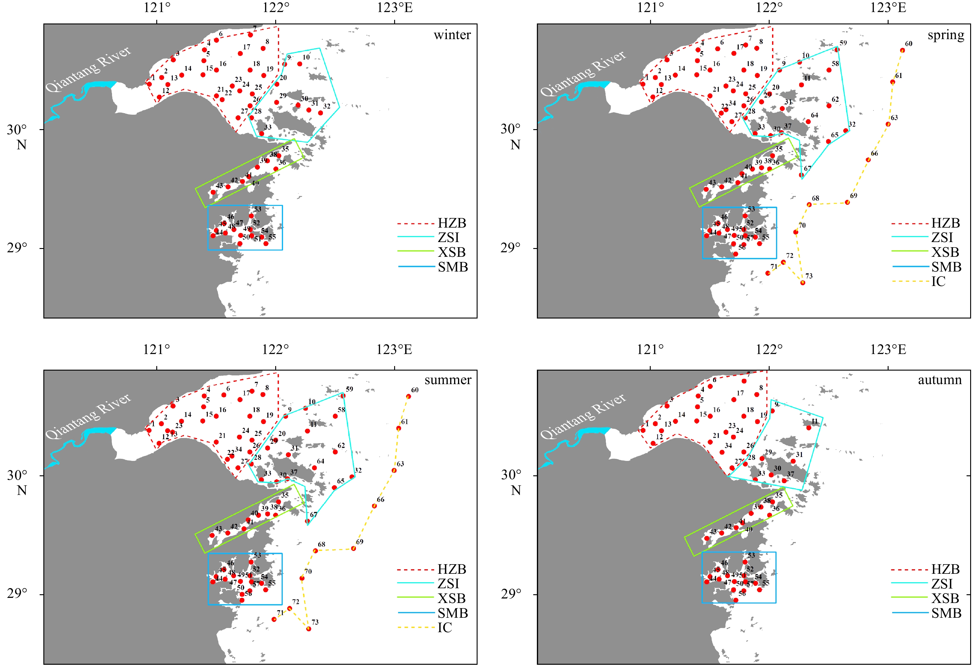
Sampling programs were carried out in February, May, August and October 2015, representing for winter, spring, summer and autumn, respectively. Due to the adjusted sampling strategy, monitoring networks in winter and autumn (52 sites) differed from that in spring and summer (73 sites) despite majority of the coastal area of northern Zhejiang has been geographically covered including HZB, ZSI, east boundary of island chain (IC), XSB and SMB (Fig. 1).

Figure  1.  Sampling sites in the coastal waters of northern Zhejiang comprised of Hangzhou Bay (HZB), Zhoushan Islands (ZSI), island chain (IC), Xiangshan Bay (XSB) and Sanmen Bay (SMB) over four seasons.

DownLoad: Full-Size Img PowerPoint

2.2 Sample collections and analyses

Water collectors attached to a CTD system (Seabird 19 Plus, USA) were employed for seawater samples collection at different layers (surface 0.5 m, 10 m, 25 m, 50 m, 100 m and bottom) according to the water depth of each station (Inspection and Quarantine of the People’s Republic of China and Standardization Administration, 2008b). Salinity (Sal), pH, water temperature (WT), suspended particulate matter (SPM), dissolved oxygen (DO), chemical oxygen demand (COD), nitrate (${{\rm {NO}}_3^-} $), nitrite (${{\rm {NO}}_2^-} $), ammonium (${{\rm {NH}}_4^+} $), phosphate (${{\rm {PO}}_4^{3-}} $), silicate (${{\rm {SiO}}_3^{2-}} $), total phosphorus (TP), total nitrogen (TN), total organic carbon (TOC) were measured via the standard methods (Inspection and Quarantine of the People’s Republic of China and Standardization Administration, 2008b). The value of each physicochemical parameter at each site was presented as the mean value of all the layers.

Phytoplankton samples were collected from bottom to surface using plankton net with a 77-μm mesh size and preserved with 5% formalin. After at least 24 h of sedimentation, samples were concentrated to 100−150 mL and then, 0.5 mL sample was uniformly siphoned onto the counting plate for counting and identification using light microscopy (Olympus bx41, Japan). Phytoplankton taxa were identified to species level at which an accurate identification could be confirmed. All the processes were conducted following the standard methods (Inspection and Quarantine of the People’s Republic of China and Standardization Administration, 2008c).

2.3 Data analysis

Prior to statistical analyses, normality tests of all the environmental parameters were conducted by Shapiro-Wilk test. Once the non-normal distributions were detected, the nonparametric Kruskal-Wallis tests were therefore applied to examine the significant variations at both spatial and seasonal scales. Mantel tests were used to examine correlations between seasonal environmental variations (Euclidean distance) and geographic distance.

Species data were lg (x+1) transformed to reduce heterogeneity. Principal coordinate analysis (PCoA) was applied to visualize spatial and seasonal dissimilarities in phytoplankton community composition based on Bray-Curtis dissimilarity matrices. Analysis of similarity (ANOSIM) was used to assess the significant dissimilarities among the four seasons and five subzones with 9999 permutations. To determine the effects of significant environmental variables (Euclidean distance) on phytoplankton community (Bray-Cutis distance), Distance-based Multivariate Linear Model (DISTLM) (Anderson, 2003) was employed. DISTLM with 999 permutations was performed to explore the relationship between significant environmental parameters and phytoplankton community structure. “Marginal tests” was used to evaluate the pure variance explained by each environmental factor and “sequential tests” to display the cumulative contribution of significant variables using forward selection procedure. In addition, Spearman’s rank correlation analysis was utilized to exhibit the dominant species (dominance Y≥0.02) (Shannon and Weaver, 1949) in relation to environmental factors via heat map.

Simple Mantel test (9999 permutations) was used to examine the correlations between phytoplankton community and geographic distance. Moreover, partial Mantel test (9999 permutations) was also used to further test it with environmental factors controlled. Distance-decay pattern was fitted with seasonal phytoplankton’s Bray-Curtis similarities against geographic distances. To examine the relative contributions of environmental factors and spatial factors in shaping phytoplankton community structure, variation partitioning analysis (VPA) (Borcard et al., 1992; Peres-Neto et al., 2006) was employed. Spatial factors, including principal coordinates of neighbour matrices (PCNM) variables and linear trend variables, were calculated by PCNM (Borcard and Legendre, 2002; Borcard et al., 2004; Dray et al., 2006). Forward selection was used to capture significant environmental, PCNM and linear trend variables through DISTLM program according to the method proposed by Blanchet et al. (2008). VPA was conducted via partial constrained analysis of principal coordinates (pCAP) with adjusted R² to quantify the total variance decomposed into four parts, the pure environmental effect, pure spatial effect, shared fraction of environmental and spatial factors, and residuals that could not be explained by the present variables.

Sampling maps and contour maps (ordinary Kriging method) of phytoplankton taxa were generated in ArcGIS 10.2. All the statistical analyses were carried out in the R environment (http://www.r-project.org).

3. Results

3.1 Tempo-spatial variations of environmental conditions

Almost all the environmental factors exhibited strong significant seasonal differences except for ${{\rm {NO}}_2^-} $, ${{\rm {NO}}_3^-} $ and TN (Table S1). WT was significantly higher in summer than other seasons (highest in summer, 31.1℃, and lowest in winter, 7.9℃) which followed predictable seasonal distribution. Sal showed weak seasonal fluctuation among spring (22.8±7.0 on average), summer (20.5±9.0 on average), and winter (20.7±6.2 on average), but higher than that in autumn (17.6±6.7 on average). DO, SPM, and COD were markedly higher in winter than in other seasons. Meanwhile, nutrients and organic maters (${{\rm {PO}}_4^{3-}} $, ${{\rm {SiO}}_3^{2-}} $, ${{\rm {NH}}_4^+} $, TP, and TOC) were substantially higher in summer compared with other seasons (Table S2).

Overall, significant spatial differences were recorded within the five subzones for all the environmental parameters except WT (Table S1, Fig. S1A). Both Sal (1.66−33.21) (Fig. S1B) and pH (7.64−8.26) (Fig. S1C) complied to the geographical-based spatial distributions with the former decreased sharply from HZB to other regions and the latter increased gradually from HZB to the offshore waters. Weak spatial differences were observed in DO with concentrations in HZB exhibiting relatively higher than other zones (Fig. S1D). COD (0.33−3.18 mg/L) (Fig. S1F), ${{\rm {NH}}_4^+} $ (0.002−0.16 mg/L) (Fig. S1K) and TOC (0.63−5.9 mg/L) (Fig. S1N) in XSB, ZSI, SMB, and IC, respectively, had no obvious spatial differences but remarkably lower than that in HZB. Moreover, the concentrations of nutrient-related factors, including SPM (9.7−5880 mg/L) (Fig. S1E), ${{\rm {PO}}_4^{3-}} $ (0.0016−0.0874 mg/L) (Fig. S1G), ${{\rm {SiO}}_3^{2-}} $ (0.285−2.999 mg/L) (Fig. S1H), ${{\rm {NO}}_3^-} $ (0.19−4.058 mg/L) (Fig. S1J), TN (0.469−4.358 mg/L) (Fig. S1L) and TP (0.0293−0.5579 mg/L) (Fig. S1M) all peaked in HZB compared with other subzones. In addition, almost all the environmental variables of the four seasons were significantly correlated with geographical distance (Table S3), suggesting that environmental gradients were spatially structured across coastal area of northern Zhejiang.

3.2 Phytoplankton community compositions

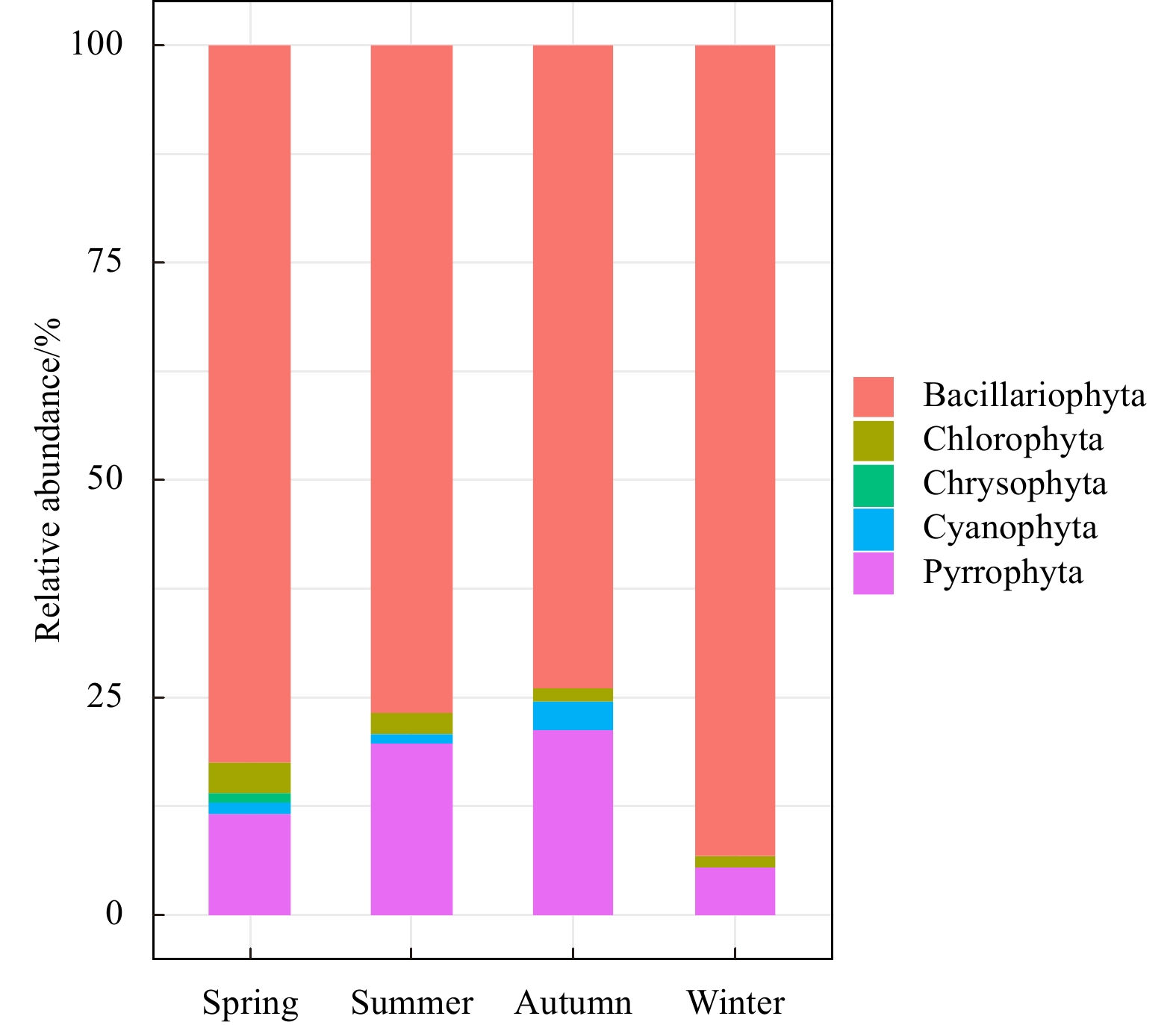
In general, a total of 136 detected species belonging to 5 phyla (Bacillariophyta, Pyrrophyta, Chlorophyta, Chrysophyta and Cyanophyta) were recorded in the four cruises. Meanwhile, regarding the seasonal dynamics, 71 species of 3 phyla, 85 species of 5 phyla, 86 species of 4 phyla and 61 species of 4 phyla were identified in winter, spring, summer and autumn, respectively. Diatoms were conceptualized as the most abundant group in terms of species composition, accounting for 82.4%, 76.7%, 73.8%, and 93% in spring, summer, autumn, and winter, respectively; followed by dinoflagellates and other groups (Fig. 2). Coscinodiscus oculs-iridis, Coscinodiscus jonesianus, and Skeletonema costatum were the major dominant species existing in all seasons.

Figure  2.  Seasonal phytoplankton community composition dynamics across sampling area.

DownLoad: Full-Size Img PowerPoint

3.3 Phytoplankton abundance

Phytoplankton abundance was markedly higher in summer ((1137087.9±3812234.7) cells/mL on average) than that in other seasons (Table S2). In spring, the most abundant area of the phytoplankton abundance covered all the zones except the central ZSI and its adjacent area around the mouth of HZB (Fig. S2A). During the autumn period, the spatial distribution resembled that in spring despite its low-value area was smaller, and the southern waters, rather than northern part, was more abundant (Fig. S2C). Meanwhile, in contrast, phytoplankton abundance peaked in HZB and decreased gradually towards the east and south in winter (Fig. S2D). Patched pattern was presented in summertime with hot spots in the extended area of eastern ZSI and the southeastern waters (Fig. S2B). The tempospatial distributions of C. oculs-iridis and C. jonesianus have almost followed the total phytoplankton abundance (Fig. S2E−L) whereas S. costatum exhibited patched distribution pattern (Figs S2M−P).

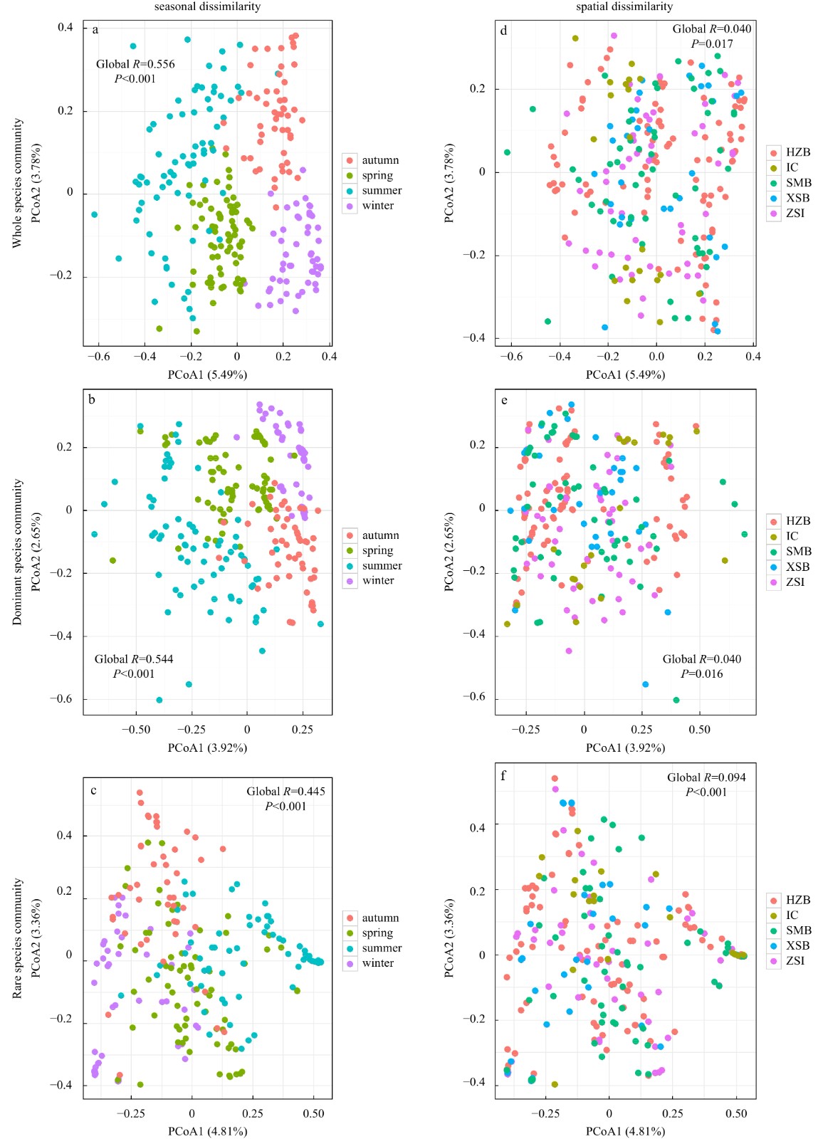
3.4 Patterns of temporal and spatial dissimilarities of the whole, the dominant and the rare communities

The PCoA plots indicated that strong seasonal differences were detected in the whole (Fig. 3a), the dominant (Fig. 3b) and the rare community (Fig. 3c), among which significant inter-seasonal differences were simultaneously observed within each of them (Tables S4 and S5). Moreover, we also found remarkable seasonal differences in each subzone (Figs S3A−E), suggesting season-to-season separation was distinguishable. Conversely, no obvious spatial differences of the three communities (Figs 3d-f) were displayed and little inter-regional differences (Tables S4 and S5) were detected in all the seasons. Similarly, relatively weak spatial differences were identified within each season (Figs S4A−D). These results emphasized that seasonal dissimilarities, rather than spatial dissimilarities, prevailed in the study area.

Figure  3.  Principal coordinate analysis (PCoA) plots of the whole community (a, d), the dominant community (b, e) and rare community (c, f) with one-way analysis of similarity (ANOSIM) visualize both seasonal (a−c) and spatial (d−f) dissimilarities. HZB: Hangzhou Bay; IC: island chain; SMB: Sanmen Bay; XSB: Xiangshan Bay; ZSI: Zhoushan Islands.

DownLoad: Full-Size Img PowerPoint

3.5 Environmental factors driving the whole community

DISTLM demonstrated that WT, DO, ${{\rm {PO}}_4^{3+}} $, and salinity were the most primary environmental factors associating with the whole phytoplankton community (Table 1, sequential tests). However, slight variations occurred in seasonal dynamics which differed among all the seasons. WT and nitrogen-related nutrients dominated in each season (Table S6−S9, sequential tests), whereas pH and nitrogen-related nutrients were the driving factors in spring and autumn (Tables S6 and S8, sequential tests), respectively.

Table  1.  Distance-based multivariate linear model against seawater chemical variables of the whole community in all the seasons

Marginal tests
Variable	Pseudo-F	P	Percent variation explained
WT	44.458	0.001	15.24
DO concentration	18.932	0.001	7.09
pH	12.062	0.001	4.64
SPM concentration	11.142	0.001	4.30
$\bf {PO_4^{3-}} $ concentration	6.077	0.001	2.39
COD	5.836	0.001	2.30
TP concentration	3.809	0.001	1.51
Sal	3.728	0.003	1.48
$\bf SiO_3^{2-} $ concentration	3.461	0.003	1.38
TN concentration	3.211	0.002	1.28
$\bf NO^-_3 $ concentration	3.048	0.005	1.21
$\bf NH_4^+ $ concentration	2.930	0.005	1.17
TOC concentration	1.715	0.069	0.69
$\bf NO_2^- $ concentration	1.481	0.136	0.59
Sequential tests
Variable	Pseudo-F	P	Cumulative variation explained
WT	44.586	0.001	15.24
DO concentration	24.823	0.001	22.98
$\bf {PO_4^{3-}} $ concentration	6.138	0.001	24.85
Sal	3.544	0.001	25.93
$\bf SiO_3^{2-} $ concentration	2.735	0.002	26.75
$\bf NO^-_3 $ concentration	2.565	0.003	27.51
TN concentration	3.077	0.001	28.42
$\bf NH_4^+ $ concentration	2.529	0.007	29.16
pH	2.389	0.009	29.86
TOC concentration	2.258	0.015	30.52
COD	2.075	0.022	31.12
TP concentration	1.805	0.055	31.64
SPM concentration	1.330	0.197	32.02
$\bf NO_2^- $ concentration	0.006	0.762	32.21
Note: Variables in bold referred to statistically significant (P<0.05). WT: water temperature; SPM: suspended particulate matter; COD: chemical oxygen demand; Sal: salinity; TOC: total organic carbon; TN: total nitrogen; TP: total phosphorus; Pseudo-F: Pseudo-F Statistics test value.

 | Show Table

DownLoad: CSV

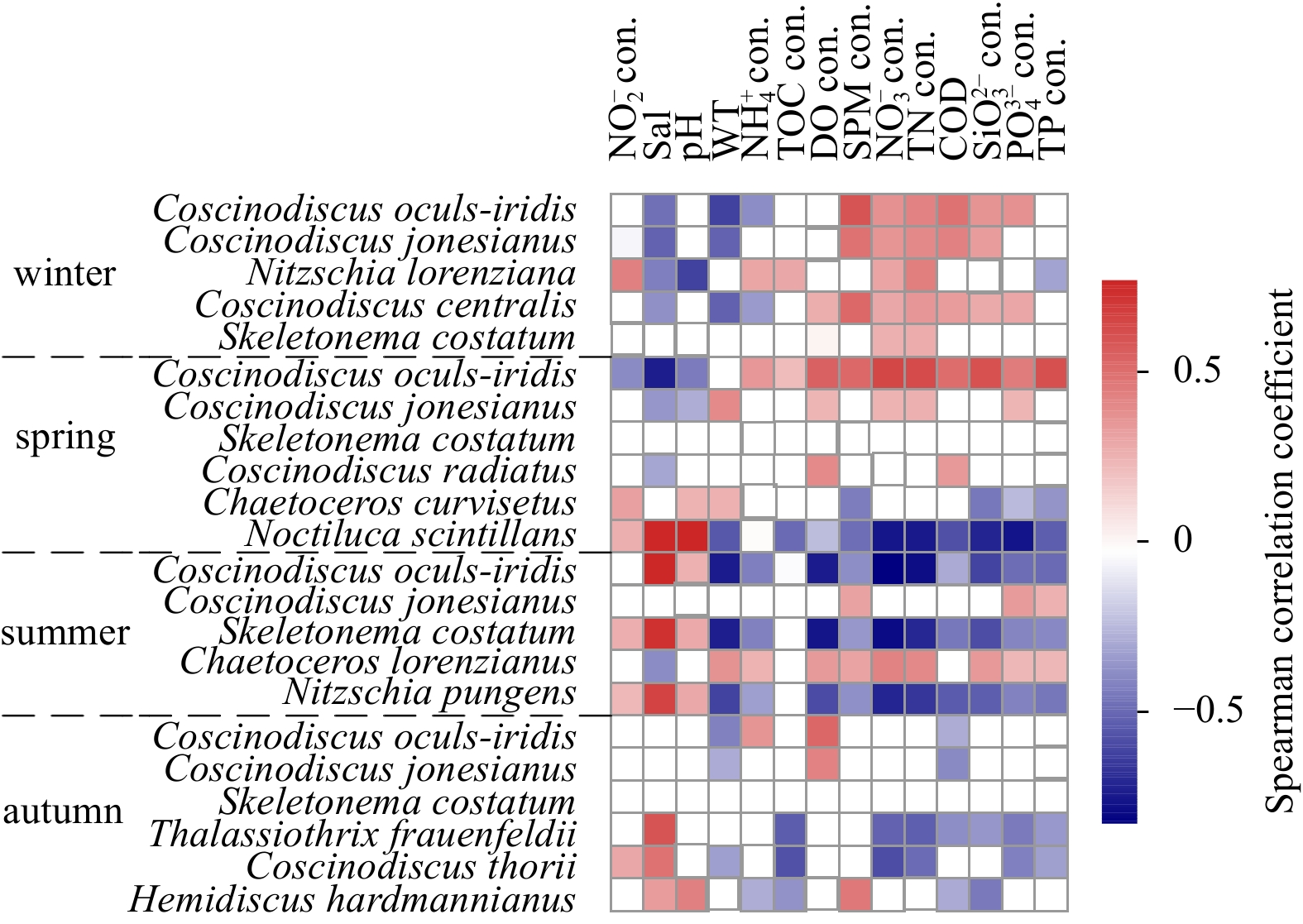
Relationships between dominant species and environmental variables in spring and winter revealed similar patterns, that was, nutrient-related factors and organic pollutants (COD, TOC) became the determinants of the whole community, especially for the three main abundant species (C. oculs-iridis, C. jonesianus and S. costatum). Meanwhile, the summertime pattern differed from that in spring and winter, with C. jonesianus only correlating positively with phosphorus-related factors, and linking C. oculs-iridis and S. costatum negatively with all nutrient-related parameters but positively with salinity and pH. In addition, random pattern was observed in autumn (Fig. 4).

Figure  4.  Heat maps illustrated Spearman’s rank correlations between seasonal dominant species and environmental parameters. WT: water temperature; Sal: salinity; TOC: total organic carbon; SPM: suspended particulate matter; TN: total nitrogen; COD: chemical oxygen demand; TP: total phosphorus; con. is the abbrevation of concentration.

DownLoad: Full-Size Img PowerPoint

3.6 Geographical distance control on the whole community

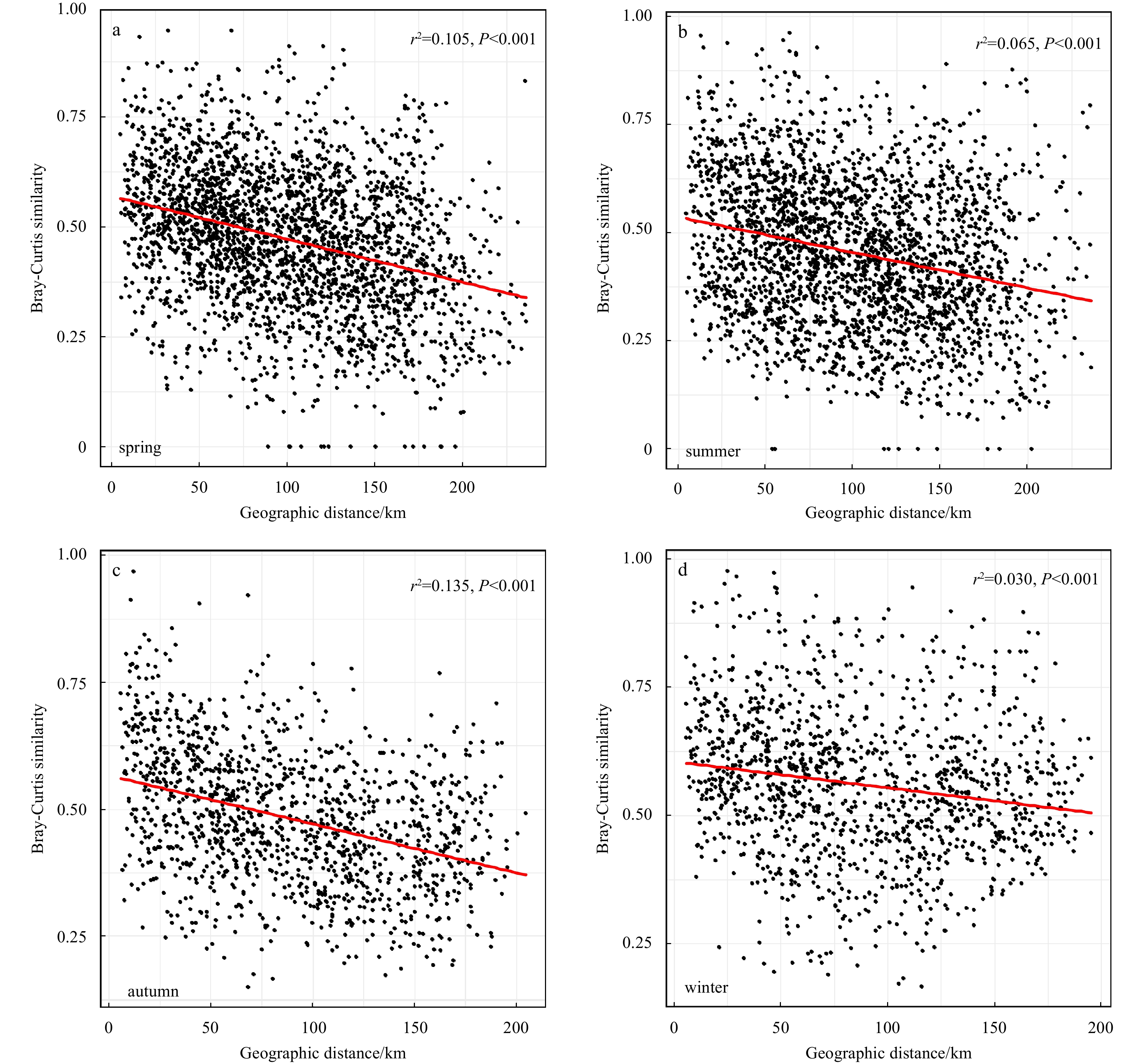
Mantel and partial Mantel tests all confirmed the significant correlations between phytoplankton community and geographical distance, irrespective of environmental variations within each season (Table 2). The whole phytoplankton community showed obvious season-to-season distance-decay patterns, with autumn (Fig. 5c, r²=0.135, P<0.001) and spring (Fig. 5a, r²=0.105, P<0.001) being relatively stronger, followed by summer (Fig. 5b, r²=0.065, P<0.001) and winter (Fig. 5d, r²=0.030, P<0.001).

Table  2.  Mantel tests showed Spearman’s rank correlations of the whole community in relation to geographic distance within the four seasons

Season	Variation source	Simple Mantel test		Controlled by	Partial Mantel test
		$\rho $	P		$\rho $	P
Spring	Geo	0.326	<0.001	Env	0.331	<0.001
Summer	Geo	0.252	<0.001	Env	0.253	<0.001
Autumn	Geo	0.370	<0.001	Env	0.373	<0.001
Winter	Geo	0.206	<0.001	Env	0.231	<0.001
Note: Geo: geographic distance; Env: environmental factors as a whole; $\rho $: correlation coefficients between pairwise distance of the whole community distance and geographic distance derived from Mantel test with 9 999 permutations.

 | Show Table

DownLoad: CSV

Figure  5.  Correlation between the whole community similarity (Bray-Curtis distance) and geographic distance between sampling sites within the four seasons. Red lines represent linear fits.

DownLoad: Full-Size Img PowerPoint

3.7 Variation partitioning of the whole community, the dominant community and the rare community

VPA revealed that environmental and spatial factors together could explained 41.7%, 36.77%, 44.07% and 13.86% of the variations of the whole species community in spring, summer, autumn, and winter, respectively (Fig. 6). Variations explained by remarkable pure environmental factors ranged from 6.83% in spring to 8.07% in autumn while the percentages of significant pure spatial effects varied from 6.33% in winter to 21.39% in autumn. The shared fractions explained by environmental and spatial effects outnumbered any pure environmental or spatial effects except that in autumn, ranging from 6.82% in winter to 20.55% in spring. Besides, over half the variations left unexplained within each season.

Figure  6.  Variation partitioning analysis of the whole species community within each season performed on environmental factors (Env) and spatial factors including linear trend variables (Trend) and principal coordinates of neighbour matrices (PCNM) variables. Values less than 0 were not shown.

DownLoad: Full-Size Img PowerPoint

Regarding the dominant and rare species communities, the joint effects of environmental and spatial factors overrode any other factors in all seasons in terms of the dominant species community (Fig. S5). Meanwhile, the rare species community was largely explained by spatial factors except that in autumn (Fig. S6).

4. Discussion

4.1 Effects of environmental conditions on phytoplankton communities and dominant species

In this study, WT, DO, ${{\rm {PO}}_4^{3-}} $, pH and Sal were identified as the key annual factors affecting phytoplankton community. Indeed, responses of phytoplankton communities to environmental variations in estuarine, coastal waters and open seas have been widely reported in previous studies (Rothenberger et al., 2009; Cloern and Dufford, 2005; Jiang et al., 2015; Mousing et al., 2016; Carstensen et al., 2015). WT is one of the most crucial physical factors influencing phytoplankton growth in marine environment (Fragoso et al., 2016). Moreover, it can also regulate seasonal dynamics of phytoplankton community succession (Dupuis and Hann, 2009). Phosphorus, especially the dissolved inorganic phosphorus, is commonly acknowledged as an essential facet for the growth of phytoplankton (Reed et al., 2016). Meanwhile, Harrison et al. (1990) has reported that the primary production in the waters off the Changjiang River Estuary (CRE) and its adjacent area were largely limited by ${{\rm {PO}}_4^{3-}} $, indicating the positive association between ${{\rm {PO}}_4^{3-}} $ and phytoplankton community. Accordingly, the photosynthesis process of phytoplankton during its fast growing period could release large amount of dissolved oxygen, leading to the high contents of DO. The significant tempospatial dynamics of pH gradient across the whole study area (Table S1, Fig. S1C) may also contribute to the variations of phytoplankton communities as Hinga (2002) reported in coastal environments at the global scale. It is no doubt that salinity is a driving parameter in shaping the seasonality of phytoplankton community (McQuoid, 2005) since they are characterized with broad salinity tolerance in the euryhaline coastal environment (Fig. S1B).

We found C. oculs-iridis, C. jonesianus and S. costatum were the main abundant species irrespective of environmental predictors varying seasonally. Strong positive correlations between species and nutrient-related parameters were observed in both spring and winter (Fig. 4). During dry and pre-wet periods, the concentrations of nutrients have been saturated due to the relatively low biological activities as well as the turbulent and eutrophic conditions. This, to large extent, facilitated diatoms to be clustered in the near-shore environments (Cloern and Dufford, 2005). Moreover, large diatoms like S. costatum and Coscinodiscus are characterized with strong capacity for nutrient absorption and assimilation to maintain a high growth rate (Philippart et al., 2000), hence accelerating nutrients consumption. However, things changed in the wet season as species associated positively with salinity and negatively with nutrient-related variables (Fig. 4). Gasiūnaitė et al. (2005) demonstrated that the massive freshwater runoff in summertime could largely decrease the abundance of diatoms. Here, in our study, abundance-rich area of the total phytoplankton assemblage as well as C. oculs-iridis (Fig. S2F) and S. costatum (Fig. S2N) were coincidently found in the open waters of eastern ZSI, indicating that hydrodynamic conditions could partly affect the spatial pattern of diatom communities. Similar findings were also reported by Zhang et al. (2018a) on microbial organisms in the same region.

4.2 Spatially structured environmental conditions shaped phytoplankton communities

Environmental conditions in this region exhibited strong spatially autocorrelated patterns within all the seasons (Table S2), implying that the seasonal dynamics of environmental gradients were spatially structured. This was also supported by the results of VPA (Fig. 6) that the variations explained by spatially structured environmental conditions outperformed any pure environmental or spatial effects (except that in autumn). Our study corresponded well with Martiny et al. (2006) who demonstrated that microbial communities were controlled by the combination of niche-based and dispersal-based processes at intermediate scales (i.e., 100−3 000 km). Consequently, it was clear that seasonal spatial heterogeneities contributed largely to the environmental variations and they sequentially shaped the biogeography of phytoplankton community composition in coastal area of northern Zhejiang. These findings were also recorded in freshwater ecosystems (Vilmi et al., 2016; Zhang et al., 2018a; Keck et al., 2018) and marine environment (Moritz et al., 2013). Furthermore, our results were especially in line with Wang et al. (2015) and Zhang et al. (2018b) whose studies claimed that bacterioplankton biogeography was also highly shaped by the joint effects of environmental- and spatial-controlled factors in the same region. Additionally, a decreasing trend of spatially structured environmental variation (from 20.55% in spring to 6.82% in winter) was detected. One possible explanation was that the seasonal differences of environmental variations and phytoplankton community have been changed (Zhang et al., 2018a). In the present study, the correlations between environmental distance and geographic distance of the five driving spatially structured environmental variables declined from spring to winter (except WT, Table S2), indicating that the seasonal environmental variations have gradually been weaker in relation to spatial variability. Moreover, given the distinct seasonal dissimilarity of phytoplankton community (Fig. 3), the spatial dissimilarities of the five subzones differed seasonally, increasing from spring to winter (Global R of ANOSIM, Fig. S3A−D). Obviously, it could be inferred that the seasonal dissimilarities of phytoplankton communities varied sharply in the study area. These results all indicated that the spatially structured environmental conditions related closely to the inherent dynamics of species living environments and the seasonal differences between communities.

4.3 Influences of spatial factors on phytoplankton communities

Previous studies have already demonstrated spatial processes as key factors in determining phytoplankton biogeography in different aquatic ecosystems (Mousing et al., 2016; Yang et al., 2018a; Ribeiro et al., 2018). In the present study, the significance of spatial factors in shaping phytoplankton communities was evidenced by Mantel tests (Tables S6−S9), and the large amounts of variation explained by pure spatial variables in VPA further confirmed it (Fig. 6). The pure spatial influences usually incorporate dispersal-related processes and unobserved abiotic factors (Liebhold et al., 2004; Liebhold and Gurevitch, 2002). Here, given the distinguishable distance-decay patterns (Fig. 5), we inferred that dispersal limitation may occur in the study area. However, some earlier researches addressed that dispersal limitation would increase with increasing spatial extent and geographic distances (Maloney and Munguia, 2011; Soininen, 2012) and dominate community structuring at continental scales (Martiny et al., 2006). Indeed, the spatial extent of our study (10−240 km) may not accordingly support the occurrence mechanism of dispersal limitation, but one thing should be noted, large microbes (e.g., diatoms and dinoflagellates) characterized with weak dispersal abilities may considerably affect by dispersal limitation. Similar findings was also reported by Astorga et al. (2012) who concluded that macroorganisms were significantly related to geographic distance compared with microorganisms. Consequently, dispersal limitation could be an ineluctable facet in structuring phytoplankton community in the study area.

Apart from the dispersal limitation, some unobserved abiotic factors may also contribute to the variations of pure spatial effects. For instance, light condition as a primary physical factor controlling phytoplankton succession has been repeatedly reported (Macintyre et al., 2002; Brunet et al., 2013; Brewin et al., 2015) in various marine environments. Moreover, it may be a crucial predictor in determining phytoplankton community, especially in the turbid and turbulent HZB where light condition became a limiting factor for phytoplankton growth (Shi et al., 2000). Nevertheless, we should also take the role of mass effects into consideration when focusing on phytoplankton biogeography. A review of Heino et al. (2015) established that because of the strong environmental gradients, mass effects were more likely to prevail in coastal zones. Generally, mass effects may involve the impacts originating from wind dispersal (Horváth et al., 2016) and the direction of water flow (Roelke et al., 2010). As we all know, intensive wind will trigger high mixing effects in water columns and hence disperse the direction of water flow, which eventually leading to high dispersal rate. Taking into account the high physical connectivity in coastal area of northern Zhejiang, of which several water masses coexists (Jiang et al., 2015), we believe that mass effects would be a potential factor attributing to phytoplankton biogeography.

Generally, a large proportion of residuals could not be explained by all the present variables. The low explanatory power may ascribe to biological gazing (Yang et al., 2018b), climate change (Harding et al., 2016; Conde et al., 2018), water circulation conditions (Jiang et al., 2015; Fragoso et al., 2016; Polikarpov et al., 2016), interspecific interactions (Yang et al., 2018b), and stochastic events (Chase and Myers, 2011) that closely related to phytoplankton community though they may weaken the direct effects from pure spatial influences. Unfortunately, these factors were not considered into, or, in other words, capable to study in this article. Given the high unexplained variations within the four seasons, it is of great importance and necessity to unravel the above-mentioned facets that potentially contribute to the unknown variations in the future researches.

5. Conclusions

This article provided a systematic research on phytoplankton biogeography in the coastal area of northern Zhejiang that integrating temporal dynamics with spatial variations. Our results demonstrated that phytoplankton community patterns were significantly subjected to seasonal dissimilarity compared with spatial dissimilarity. Phytoplankton biogeography was determined by spatially structured environmental condition with spatial process, however, also being a crucial factor. In addition, future investigations should be concentrated more on the effects of biological gazing, climate change, hydrodynamic conditions, and interspecific interactions that resulting from the large amounts of unexplained variations. Furthermore, long-term dataset is still expected to be utilized to continuously improve our work despite the current study have temporally covered an annual scale.