A dedicated GPS buoy is designed for calibration and validation (Cal/Val) of satellite altimeters since 2014. In order to evaluate the accuracy of the sea surface height (SSH) measured by the GPS buoy, twelve campaigns have been done within China sea area between 2014 and 2021. In six of these campaigns, two static Global Navigation Satellite System stations were installed at distances of <1 km and 19 km from the buoy to assess how the baseline length influenced the derived SSH from the buoy solutions. The GPS buoy data was processed using the GAMIT/GLOBK software+TRACK module and CSRS-PPP tool to achieve the SSH. The SSH was compared with conventionally tide gauge (TG) data to evaluate the accuracy of the buoy with the standard deviation of the height element. The results showed that the difference in the standard deviation of the SSH from the buoy and the TG was less than 16 mm. The SSHs processed with different ephemeris (Ultra-Rapid, Rapid, Final) were not significantly different. When the baseline length was 19 km, the SSH solution of the GPS buoy performed well, with standard bias of less than 26 mm between the heights measured by the buoy and TG, meaning that the buoy could be used for Cal/Val of altimeters. The bias between the Canadian Spatial Reference System-precise point positioning tool and the TRACK varied a lot, and some of them were over 130 mm. This deemed too high to be useful for Cal/Val of satellite altimeters. Moreover, the GPS buoy solutions processed by GAMIT/GLOBK software+TRACK module were used for in-orbit Cal/Val of HY-2B/C satellites in ten campaigns. The SSH and significant wave height of the altimeters showed good agreements with the GPS buoy solutions.
The Bjerknes feedback is a positive feedback loop including the response of the equatorial zonal wind to the sea surface temperature (SST), the response of the thermocline to equatorial zonal winds and the response of the SST to variations in the thermocline (Bjerknes, 1969). Although the Bjerknes feedback was first used to explain air-sea interactions in the Pacific Ocean (Neelin et al., 1998; Zelle et al., 2004; Xiang et al., 2012; Zhu et al., 2015, 2021; Dong and McPhaden, 2018; Yuan et al., 2020), it has also been shown to be a key mechanism in the formation and development of the two major interannual ocean-atmosphere coupled modes in the Indian Ocean (Saji et al., 1999; Xie et al., 2010): the Indian Ocean Dipole (IOD) (Saji et al., 1999) and the Indian Ocean Basin (IOB) (Cadet, 1985) modes. Among the three components of the Bjerknes feedback, the response of the SST to variations in the thermocline, which is referred to as the thermocline-SST feedback, contributes the most to the intensity of the Bjerknes feedback (Jin et al., 2006). It is also a key process in the Bjerknes feedback influencing IOD and El Niño Southern Ocean events (Cai et al., 2013; Ren and Jin, 2013; Ng et al., 2014, 2018; Kim et al., 2017; Zhu et al., 2021).
The strength of the thermocline-SST feedback depends on the mean state of the tropical Indian Ocean. The vertical velocity and the depth of the thermocline are the two most important factors. The subsurface temperature anomaly, which is induced by fluctuations in the thermocline depth, is transported upward by upwelling until it reaches the surface (Zelle et al., 2004). When upwelling is weak and there is a deep thermocline, the weak vertical advection cannot efficiently transfer the subsurface temperature anomaly to the surface. In addition, the response of the SST anomaly to variations in the depth of the thermocline is delayed as a result of the greater distance between the thermocline and the sea surface. The thermocline-SST feedback is therefore weakened (Zelle et al., 2004; Zhu et al., 2015). By contrast, a shallower thermocline and a greater mean vertical upwelling velocity favor a strong thermocline-SST feedback (Liu et al., 2011).
The strength of the thermocline-SST feedback has changed significantly in recent decades in response to changes in the mean state of the oceans. For example, the climatological thermocline in the southeastern Indian Ocean has shallowed under global warming and therefore the response of the SST to the thermocline has increased. This has contributed to the increase in the frequency of the IOD in the second half of the twentieth century (Cai et al., 2013) and the emergence of an unseasonable IOD in the last 30 a (Du et al., 2013). The thermocline-SST feedback in the southwestern Indian Ocean is a key factor in the development of the IOB. The IOB and the resultant Indian Ocean capacitor effect have intensified since 1970 and will continue to intensify under global warming as the thermocline-SST feedback strengthens as a result of shallowing of the local thermocline (Xie et al., 2010; Zheng et al., 2010).
The global SST underwent rapid warming in the second half of the twentieth century. The rate of global warming then slowed and there was a hiatus in global warming in the early twenty-first century (Easterling and Wehner, 2009; Kerr, 2009; Stan et al., 2017). The trend of the depth of the thermocline in this period of hiatus is distinct from that in the period of rapid warming, when notable subsurface cooling was accompanied by a shallowing thermocline (Han et al., 2006; Trenary and Han, 2008). By contrast, abrupt subsurface warming and a deepening thermocline were detected when the surface warming of the tropical Indian Ocean stalled in the hiatus period (Lee et al., 2015; Nieves et al., 2015). Because the depth of the thermocline can greatly affect the thermocline-SST feedback, it is reasonable to hypothesize that a reversed trend in the depth of the thermocline could induce significant changes in thermocline-SST feedback in the Indian Ocean. However, the variation in the thermocline-SST feedback in this time period is not clear at the present time. We therefore analyzed the variation in the thermocline-SST feedback over the last 40 a and discuss the underlying mechanisms.
2.
Data
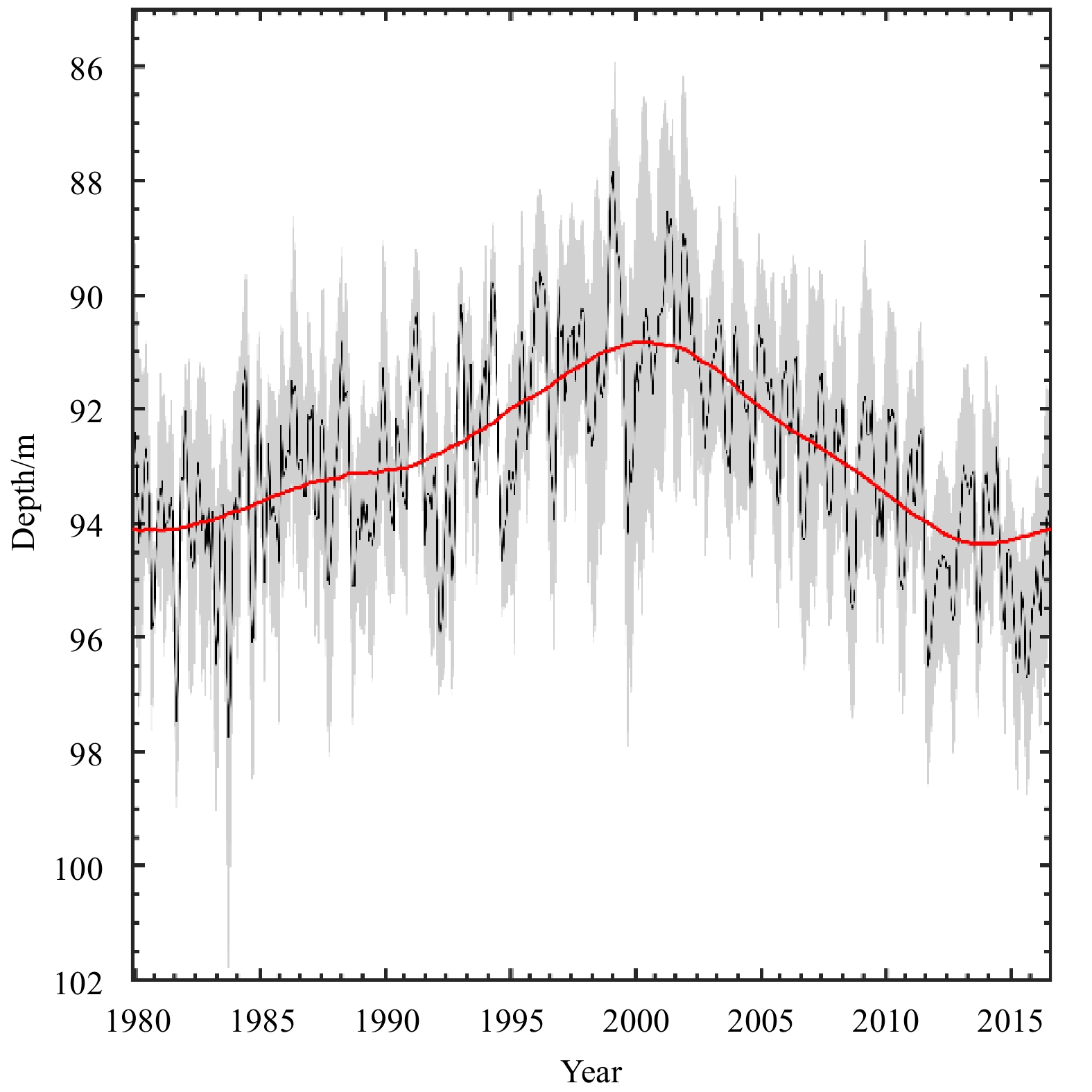
To ensure the robustness of the results, four sea temperature datasets are used for the SST and thermocline depth calculations. The depth of the 20°C isotherm is used as a proxy for the depth of the thermocline. The four datasets are: the UK Meteorological Office Hadley Center EN 4.2.1 quality-controlled ocean temperature dataset (Good et al., 2013) from 1900 to the present day; the Simple Ocean Data Assimilation version 3.4.2 (SODA 3.4.2) reanalysis dataset from 1980 to 2019 (Carton and Giese, 2008); the Operational Ocean Reanalysis System 4 (ORAS4) reanalysis dataset from 1958 to 2016 (Balmaseda et al., 2013); and the National Centers for Environmental Prediction Global Ocean Data Assimilation System (GODAS) dataset from 1980 to 2019 (Behringer and Xue, 2004). These datasets successfully capture the reversed trend in the depth of the thermocline between the rapid warming period and hiatus period (Fig. 1). In addition, surface wind field of NCEP/NCAR Reanalysis Monthly Means dataset from 1948 to 2019 (Kalnay et al., 1996) was used to analyze the zonal wind and wind stress curl. Considering the time range of these datasets and the purpose of this study, we select the last 40 a (1980–2019; 1980–2016 for the ORAS4 dataset) to study the decadal variations in the thermocline-SST feedback.
Figure
1.
Decadal variation in the depth of the thermocline in the tropical Indian Ocean (15°S–15°N, 40°–120°E). The solid black line and the gray shading are the mean and standard deviation, respectively, of the thermocline depth calculated using the GODAS, SODA 3.4.2, ORAS4 and EN 4.2.1 datasets. The solid red line is the nine-year running mean of the average thermocline depth.
The correlation and regression coefficient between the SST and thermocline depth are calculated based on their monthly anomalies. The thermocline depth anomalies and SST anomalies for each month are computed by subtracting the corresponding monthly climatology. The decadal variations in the correlation and regression coefficients are calculated using the four datasets and the result is consistent among all four datasets. The 20°C-isothermal depth (D20 hereafter) is used as a proxy for thermocline depth.
3.
Decadal variations in the thermocline-SST feedback
We first analyzed the seasonal variation in the correlation coefficient between the D20 anomaly and SST anomaly in the tropical Indian Ocean. Spring, summer, autumn and winter are represented by the four typical months of April, July, October and November, respectively. Figure 2 shows that the regions with the strongest positive correlation between the D20 anomaly and SST anomaly are mainly located in the southeastern and the southwestern Indian Ocean. The positive correlation in the southeastern Indian Ocean is most significant in summer and autumn, whereas that in the southwestern Indian Ocean is strongest in winter and spring. These results are consistent with previous studies (Annamalai et al., 2003). These two regions are crucial in the development of air-sea coupled phenomena in the Indian Ocean. The thermocline-SST feedback in the southwestern Indian Ocean plays a key part in the formation of the IOB and can modulate the decadal variation of the IOB and the subsequent Indian Ocean capacitor effect (Xie et al., 2010). The southeastern Indian Ocean is the region with the strongest anomalies in both the ocean and atmosphere. The thermocline-SST feedback in this region is crucial in the development and change in decadal frequency of the IOD (Cai et al., 2013). We therefore selected the southeastern Indian Ocean (0°–10°S, 90°–110°E) and the southwestern Indian Ocean (8°–14°S, 65°–80°E) for specific analysis on the interdecadal changes in the thermocline-SST feedback.
Figure
2.
Seasonal variation in the correlation coefficient between the D20 anomaly and SST anomaly in the Indian Ocean in January (a), April (b), July (c) and October (d) based on the SODA 3.4.2 dataset. Values exceeding the 95% significance level are shaded. The black rectangles denote the location of the southwestern Indian Ocean and the southeastern Indian Ocean.
The correlation coefficient between the D20 anomaly and the SST anomaly reflects the synchronicity of their interannual variations. It is an important indicator used to measure the significance of the thermocline-SST feedback. Figures 3a and b show the 19-year sliding correlation coefficient between the D20 anomaly and the SST anomaly in the southeastern and southwestern Indian Ocean. The years in Fig. 3 denote the centers of the sliding windows (e.g., 2000 represents the correlation in the 19-year sliding window of 1991–2009). The results in Fig. 3a show that there is a significant positive correlation from July to December in the southeastern Indian Ocean that peaks in the autumn. The correlation coefficient between the D20 anomaly and the SST anomaly shows pronounced decadal variations in these months. The correlation coefficient shows a rapid increase before about 2002 from about 0.6 to >0.8 and then decreases. The positive correlation persists through winter and spring in the southwestern Indian Ocean and the decadal variation is the most significant in these two seasons (Fig. 3b). Similar to the southeastern Indian Ocean, the decadal trend of the southwestern Indian Ocean reversed at the start of this century and the correlation coefficient was greater than 0.8. We compared the decadal trends of the correlation in their peak months based on different datasets in Figs 3c and d. As different datasets use different models and methods in data assimilation, the results of them are slightly different. Argo data has been added to all the four data sets since 2000, which improved the data quality considerably. The four datasets all captured the basic characteristics of the decadal variations in the correlation coefficient in the two regions. It is also evident that our results showed better consistency after 2000 (Figs 3c and d).
Figure
3.
Decadal variation in the correlation coefficient between the D20 anomaly and SST anomaly in the southeastern (a) and the southwestern (b) Indian Ocean based on the SODA 3.4.2 dataset (values exceeding the 95% significance level are shaded); and the decadal variations of the correlation coefficient between the D20 anomaly and SST anomaly in the southeastern Indian Ocean during October (c) and the southwestern Indian Ocean during April (d) based on multiple datasets.
In addition to the correlation coefficient, the regression coefficient between the SST anomaly and the D20 anomaly is also an important indicator used to measure the significance of the thermocline-SST feedback. The value of the regression coefficient represents the intensity of the response of the SST anomaly to the D20. A larger regression coefficient implies a greater SST response to a unit of change in the D20.
To further analyze the decadal variation in the thermocline-SST feedback, we compared the regression coefficients and correlation coefficients of the SST anomaly and the D20 anomaly during the study period. We selected the months with the strongest correlation between D20 anomaly and SST anomaly in the tropical Indian Ocean—that is, July–November in the tropical southeastern Indian Ocean and April–June in the tropical southwestern Indian Ocean. Figure 4 shows that the decadal variations in the correlation and regression coefficients are highly consistent with each other. They both first strengthened and then weakened during the study period. The thermocline-SST feedback was therefore strongest at the beginning of the twenty-first century from both the perspective of the synchronicity and the intensity of the response between changes of D20 anomaly and SST anomaly.
Figure
4.
Correlation coefficient (blue line) and regression coefficient (orange line) of the D20 anomaly and SST anomaly in October in the southeastern Indian Ocean (a) and in April in the southwestern Indian Ocean (b) based on the SODA 3.4.2 dataset.
4.
Mechanisms of the decadal variations in the thermocline-SST feedback
Previous studies have shown that D20 and vertical velocity are the two most important factors in the variation of the thermocline-SST feedback. This section explores their changes during the study period and examines their contribution to the decadal variation in the thermocline-SST feedback.
The decadal variations of D20 and the correlation between D20 anomaly and SST anomaly are in good agreement in the seasons with a significant thermocline-SST feedback. The thermocline rises before 2002 and deepens in the following years (Fig. 5). When the thermocline rises, it is closer to the sea surface and therefore variations could influence the SST more directly and quickly, which favors an increase in the thermocline-SST feedback. The D20 in the southeastern Indian Ocean is shallowest in about 2002 (Fig. 5a), which coincides with the time when the thermocline-SST feedback is strongest in the study period (Fig. 3a). The thermocline in the southwestern Indian Ocean rises before 2003 and deepens in the following years (Fig. 5b), which is also consistent with the variation in the correlation between D20 anomaly and SST anomaly in this region (Fig. 3b). For the same reason as Figs 3c and d, the results of the four data sets are slightly different in Figs 5c and d. The four datasets all captured the basic characteristics of the decadal variations of D20 in the two regions. The results also showed better consistency after 2000. These results confirm the importance of D20 in the decadal variation of the thermocline-SST feedback. Besides, decadal variations in D20 are also important for the equatorial zonal wind-thermocline feedback, which is another component of Bjerkens feedback (Bjerknes, 1969). This feedback also strengthens when D20 gets shallower. Because the zonal wind could force the thermocline more directly when thermocline is closer to the sea surface.
Figure
5.
Decadal variation in the thermocline depth in the southeastern (a) and the southwestern (b) Indian Ocean based on the SODA 3.4.2 dataset (the values of correlation coefficients between D20 anomaly and SST anomaly exceeding the 95% significance level are shaded as in Figs 3a and b); and decadal variations in the D20 anomaly in the southeastern Indian Ocean during October (c) and the southwestern Indian Ocean during April (d) based on multiple datasets. D20 anomaly less than 0 represents a shallower thermocline.
Although the decadal variations of D20 and the intensity of the thermocline-SST feedback are generally consistent, there are some differences in certain months. For example, the correlation coefficient between D20 anomaly and SST anomaly in the southwestern Indian Ocean shows significant decadal changes in February and March and peaks in about 2003 (Fig. 3b). However, the variation of D20 is weak in these months (Fig. 5b). This implies that thermocline is not the only contributor to variations in the thermocline-SST feedback.
To find the cause of this phenomenon, we analyzed the decadal changes in upwelling in the region. Because upwelling is strongest at about 40–60 m (Figs 6a and b), we plot the decadal variation in upwelling within this depth range (Figs 6c and d). The decadal variation of D20 in the southeastern Indian Ocean does not agree completely with the variation in the thermocline-SST feedback. Upwelling has experienced a weakening-strengthening-weakening trend in summer in recent decades (Fig. 6a). The thermocline-SST feedback increased before 1995 (Fig. 3a), but local upwelling weakened (Figs 6a and c). During this period, the feedback intensity was mainly controlled by the variation of the D20. The climatology upwelling of the background field is in summer, thus the temperature anomalies caused by thermocline fluctuations can be still effectively transported to the surface layer even if the intensity of upwelling changes slightly. After 1995, the variation of upwelling was consistent with that of the feedback intensity.
Figure
6.
Decadal variation in the vertical velocity in the southeastern Indian Ocean from June to November (a) and the southwestern Indian Ocean from January to May (b) based on the GODAS dataset; and decadal variations in the vertical velocity at 40–60 m in the southeastern (c) and the southwestern (d) Indian Ocean based on the GODAS dataset. The values of correlation coefficients between D20 anomaly and SST anomaly exceeding the 95% significance level are shaded (as in Figs 3a and b).
In the southwestern Indian Ocean, the decadal variation in the vertical velocity is greatest in February–March (Fig. 6d) and leads the variation in the thermocline depth for two months. The decadal variation in the thermocline-SST feedback in these months is therefore induced by variations in upwelling rather than D20. Enhanced upwelling helps to bring the subsurface sea temperature anomalies to the surface and strengthens the correlation between D20 anomaly and SST anomaly. The situation is reversed for weakened upwelling. The strength of upwelling in April–June is stable on a decadal timescale. Consequently, the decadal variation in thermocline-SST feedback is influenced by variations of D20 in these months. This is because the D20 does not change synchronously with the vertical velocity in the southwestern Indian Ocean, but responds to the gradient in vertical velocity with respect to time, which lags the vertical velocity by about two months (Hermes and Reason, 2008).
From the above analysis, we conclude that the intensity of upwelling and D20 are the key factors that affect the decadal variation in the thermocline-SST feedback. What are the causes for the decadal variation in upwelling and D20? To answer this question, we analyzed the relationship between the D20 and surface wind on decadal time scale. We select September and May, when the D20 variation is most robust, for the southeastern and southwestern Indian Ocean, respectively (Figs 5a and b). Results show that the D20 in southeastern Indian Ocean is significantly correlated with the equatorial zonal wind (Fig. 7a). Meanwhile, the D20 of southwestern Indian Ocean is mainly associated with the wind stress curl variation in the southeastern Indian Ocean (8°–16°S, 85°–105°E) (Fig. 7b).
Figure
7.
Correlation coefficient between decadal variations in D20 anomaly of southeastern Indian Ocean in September and zonal wind in August (a), between decadal variations in D20 anomaly of southwestern Indian Ocean in May and the wind stress curl in February (b); and lead-lag correlation coefficient between equatorial zonal wind in August and the D20 anomaly (upwelling anomaly) in the southeastern Indian Ocean (c), between wind stress curl in the southeastern Indian Ocean in February and the D20 anomaly (upwelling anomaly) in the southwestern Indian Ocean (d). In a and b, the black box denotes the location of the equatorial zonal wind (5°N–8°S, 55°–90°E) and the critical areas of wind stress curl (8°–16°S, 85°–105°E), respectively. Values exceeding the 95% significance level are shaded. In c and d, lag>0 denotes the variation of D20 and upwelling lags behind the equatorial zonal wind and wind stress curl. Among them, temperature data, vertical velocity data and wind field data are based on EN4.2.1, GODAS and NCEP, respectively.
We further examine the relationship between the D20 and surface based on lead-lag correlations (Figs 7c and d). The D20 and upwelling in southeastern Indian Ocean are best correlated with the equatorial zonal wind at the same month, with correlation coefficients of about 0.8 (Fig. 7c). The equatorial zonal wind anomaly can lead to the anomalous horizonal advection, which directly induce opposite changes in the vertical velocity of the eastern and western equatorial Indian Ocean and modulate the D20. However, the variations of upwelling and D20 of southwestern Indian Ocean lag that of the wind stress curl for 2 months and 4 months, respectively (Fig. 7d). Wind stress curl in the southeastern Indian Ocean could influence the local Ekman pumping, and the D20 varies accordingly. The signal is transmitted to southwestern Indian Ocean via Rossby waves. As suggested by Xie et al. (2002), this process takes about 2 months. The D20 needs another 2 months to adjust to the upwelling change as discussed above, thus there is a notable delay between thermocline variation and that of wind stress curl.
5.
Summary
We analyzed the decadal variation in the thermocline-SST feedback in the tropical Indian Ocean during the rapid warming period and the global warming hiatus period and discussed its underlying mechanisms. The results for the last 40 a show that the thermocline-SST feedback first strengthened and then weakened and its intensity peaked at the beginning of the twenty-first century.
The thermocline-SST feedback was strongest in the southeastern and southwestern Indian Ocean, where there was significant feedback in summer-autumn and winter-spring, respectively. In these regions, the thermocline depth and upwelling both contributed to the variations in the thermocline-SST feedback, but their relative importance varies with season. The variation of D20 in the southeastern Indian Ocean is highly consistent with the strength of thermocline-SST feedback on a decadal scale. The feedback strengthens when the thermocline rises and weakens when it deepens. By contrast, the decadal variation of the thermocline-SST feedback in the southwestern Indian Ocean is mainly forced by the intensity of upwelling in February–March and controlled by variations in the D20 in April–June. The D20 and upwelling of southeastern Indian Ocean are mainly affected by the equatorial zonal wind. Whereas the wind stress curl over the southeastern Indian Ocean is the main factor affecting D20 and upwelling in southwestern Indian Ocean. Thermocline and upwelling in southeastern Indian Ocean respond quickly to zonal wind without significant delay, while the thermocline and upwelling in southwestern Indian Ocean lag the wind stress curl by 4 and 2 months, respectively.
The thermocline-SST feedback has experienced pronounced decadal variation in recent decades. These changes will inevitably affect the overall strength of the Bjerknes feedback and therefore influence the air-sea coupling modes of the Indian Ocean. The results of this study will help us to understand the ocean surface-subsurface interactions in the Indian Ocean and improve the accuracy of regional climate prediction.
Ardalan A A, Jazireeyan I, Abdi N, et al. 2018. Evaluation of SARAL/AltiKa performance using GNSS/IMU equipped buoy in Sajafi, Imam Hassan and Kangan Ports. Advances in Space Research, 61(6): 1537–1545. doi: 10.1016/j.asr.2018.01.001
Babu K N, Shukla A K, Suchandra A B, et al. 2015. Absolute calibration of SARAL/AltiKa in Kavaratti during its initial calibration-validation phase. Marine Geodesy, 38(S1): 156–170. doi: 10.1080/01490419.2015.1045639
Bonnefond P, Exertier P, Laurain O, et al. 2013. GPS-based sea level measurements to help the characterization of land contamination in coastal areas. Advances in Space Research, 51(8): 1383–1399. doi: 10.1016/j.asr.2012.07.007
Cancet M, Bijac S, Chimot J, et al. 2013. Regional in situ validation of satellite altimeters: calibration and cross-calibration results at the Corsican sites. Advances in Space Research, 51(8): 1400–1417. doi: 10.1016/j.asr.2012.06.017
Chen Xiaoming, Allison T, Cao Wei, et al. 2011. Trimble RTX, an innovative new approach for network RTK. In: Proceedings of the 24th International Technical Meeting of the Satellite Division of the Institute of Navigation. Portland, OR: Oregon Convention center: 2214–2219
Chen Chuntao, Zhai Wanlin, Yan Longhao, et al. 2014. Assessment of the GPS buoy accuracy for altimeter sea surface height calibration. In: Proceedings of the 2014 IEEE Geoscience and Remote Sensing Symposium. Quebec City, Canada: IEEE, 3101–3104. doi: 10.1109/IGARSS.2014.6947133
Chen Chuntao, Zhu Jianhua, Ma Chaofei, et al. 2021. Preliminary calibration results of the HY-2B altimeter’s SSH at China’s Wanshan calibration site. Acta Oceanologica Sinica, 40(5): 129–140. doi: 10.1007/s13131-021-1745-y
Chen Chuntao, Zhu Jianhua, Zhai Wanlin, et al. 2019. Absolute calibration of HY-2A and Jason-2 altimeters for sea surface height using GPS buoy in Qinglan, China. Journal of Oceanology and Limnology, 37(5): 1533–1541. doi: 10.1007/s00343-019-8216-8
Crétaux J F, Bergé-Nguyen M, Calmant S, et al. 2018. Absolute calibration or validation of the altimeters on the Sentinel-3A and the Jason-3 over Lake Issykkul (Kyrgyzstan). Remote Sensing, 10(11): 1679. doi: 10.3390/rs10111679
Dawidowicz K, Krzan G. 2014. Coordinate estimation accuracy of static precise point positioning using on-line PPP service, a case study. Acta Geodaetica et Geophysica, 49(1): 37–55. doi: 10.1007/s40328-013-0038-0
Dong Xiaojun, Woodworth P, Moore P, et al. 2002. Absolute calibration of the TOPEX/POSEIDON altimeters using UK tide gauges, GPS, and precise, local geoid-differences. Marine Geodesy, 25(3): 189–204. doi: 10.1080/01490410290051527
Estey L H, Meertens C M. 1999. TEQC: The multi-purpose toolkit for GPS/GLONASS data. GPS Solutions, 3(1): 42–49. doi: 10.1007/pl00012778
Fu L L, Christensen E J, Yamarone C A Jr, et al. 1994. TOPEX/POSEIDON mission overview. Journal of Geophysical Research, 99(C12): 24369–24381. doi: 10.1029/94JC01761
Geng Jianghui, Chen Xingyu, Pan Yuanxin, et al. 2019. PRIDE PPP-AR: an open-source software for GPS PPP ambiguity resolution. GPS solutions, 23(4): 91
Herring T A. 2012. TRACK GPS Kinematic Positioning Program, Version 1.07. Cambridge, MA: Massachusetts Institute of Technology
Herring T A, King R W, Folyd M A, et al. 2018. Introduction to GAMIT/GLOBK Release 10.7. Massachusetts Institute of Technology. http://www-gpsg.mit.edu/gg/docs/Intro_GG.pdf[2018-06-07/2018-06-20]
Jia Zhige, Chen Zhengsong, Wang Dijin, et al. 2014. The quality test of TOPCON NET-G3A GNSS receiver. Applied Mechanics and Materials, 511–512: 290–293, doi: 10.4028/www.scientific.net/AMM.511-512.290
Jiang Xingwei, Jia Yongjun, Zhang Youguang. 2019. Measurement analyses and evaluations of sea-level heights using the HY-2A satellite’s radar altimeter. Acta Oceanologica Sinica, 38(11): 134–139. doi: 10.1007/s13131-019-1503-6
Jin Honglin, Gao Yuan, Su Xiaoning, et al. 2019. Contemporary crustal tectonic movement in the southern Sichuan-Yunnan block based on dense GPS observation data. Earth and Planetary Physics, 3(1): 53–61. doi: 10.26464/epp2019006
Kato T, Terada Y, Nagai T, et al. 2010. Tsunami monitoring system using GPS buoy—Present status and outlook. In: 2010 IEEE International Geoscience and Remote Sensing Symposium. Honolulu, HI, USA: IEEE, 3043–3046. doi: 10.1109/IGARSS.2010.5654449
Li Fei, Zhang Qingchuan, Zhang Shengkai, et al. 2020. Evaluation of spatio-temporal characteristics of different zenith tropospheric delay models in Antarctica. Radio Science, 55(5): e2019RS006909. doi: 10.1029/2019RS006909
Lin Yen-Pin, Huang Ching-Jer, Chen Sheng-Hsueh, et al. 2017. Development of a GNSS buoy for monitoring water surface elevations in estuaries and coastal areas. Sensors, 17(1): 172. doi: 10.3390/s17010172
Liu Yalong, Tang Junwu, Zhu Jianhua, et al. 2014. An improved method of absolute calibration to satellite altimeter: A case study in the Yellow Sea, China. Acta Oceanologica Sinica, 33(5): 103–112. doi: 10.1007/s13131-014-0476-8
Martinez-Benjamin J J, Martinez-Garcia M, Lopez S G, et al. 2004. Ibiza absolute calibration experiment: survey and preliminary results. Marine Geodesy, 27(3–4): 657–681, doi: 10.1080/01490410490883342
Ménard Y, Jeansou E, Vincent P. 1994. Calibration of the TOPEX/POSEIDON altimeters at Lampedusa: additional results at harvest. Journal of Geophysical Research: Oceans, 99(C12): 24487–24504. doi: 10.1029/94JC01300
Salleh A M, Daud M E. 2015. Development of a GPS buoy for ocean surface monitoring: initial results. World Academy of Science, Engineering and Technology, 9(6): 769–772,
Stewart R H. 2008. Introduction to Physical Oceanography. Texas: Texas A&M University
Tang Yuxiang, Sun Hongliang, Hu Xiaomin, et al. 2008. GB/T 12763.2-2007. Specifications for oceanographic survey-Part 2: Marine hydrographic observation (in Chinese). Beijing: Standards Press of China
Wang Nazi, Xu Tianhe, Gao Fan, et al. 2018. Sea level estimation based on GNSS dual-frequency carrier phase linear combinations and SNR. Remote Sensing, 10: 470,
Watson C S. 2005. Satellite altimeter calibration and validation using GPS buoy technology [dissertation]. Hobart: University of Tasmania
Watson C, Coleman R, Handsworth R. 2008. Coastal tide gauge calibration: A case study at Macquarie Island using GPS buoy techniques. Journal of Coastal Research, 2008(244): 1071–1079. doi: 10.2112/07-0844.1
Xu Xiyu, Xu Ke, Shen Hua, et al. 2016. Sea surface height and significant wave height calibration methodology by a GNSS buoy campaign for HY-2A altimeter. IEEE Journal of Selected Topics in Applied Earth Observations and Remote Sensing, 9(11): 5252–5261. doi: 10.1109/JSTARS.2016.2584626
Zhai Wanlin, Zhu Jianhua, Chen Chuntao, et al. 2019. Calibration of HY-2A satellite altimeter based on GPS bouy. In: Proceedings of the 2019 IEEE International Geoscience and Remote Sensing Symposium. Yokohama, Tokyo: IEEE, 8300–8303. doi: 10.1109/IGARSS.2019.8900272
Zhai Wanlin, Zhu Jianhua, Fan Xiaohui, et al. 2021. Preliminary calibration results for Jason-3 and Sentinel-3 altimeters in the Wanshan Islands. Journal of Oceanology and Limnology, 39(2): 458–471. doi: 10.1007/s00343-020-9251-1
Zhai Wanlin, Zhu Jianhua, Lin Mingsen, et al. 2022. GNSS data processing and validation of the altimeter zenith wet delay around the Wanshan Calibration Site. Remote Sensing, 14, 6235,
Zhou Boye, Watson C, Legresy B, et al. 2020. GNSS/INS-equipped buoys for altimetry validation: Lessons learnt and new directions from the Bass Strait validation facility. Remote Sensing, 12(18): 3001. doi: 10.3390/rs12183001
Zumberge J F, Heflin M B, Jefferson D C, et al. 1997. Precise point positioning for the efficient and robust analysis of GPS data from large networks. Journal of Geophysical Research: Solid Earth, 102(B3): 5005–5017. doi: 10.1029/96JB03860
Zuo Xianqing, Bu Jinwei, Li Xiangxin, et al. 2019. The quality analysis of GNSS satellite positioning data. Cluster Computing, 22(3): 6693–6708. doi: 10.1007/s10586-018-2524-1
Figure 1. GPS buoy deployment in the ZW2 campaign. The buoy was moored near the wharf of Zhiwan Island. The TG and the static GPS station were placed on the island.
Figure 2. Twelve campaigns conducted from 2014 to 2021. Campaigns 2, 4–7, 10–12 in Table 1 are shown in the top-left figure. In Campaigns 1–3 and 8–9, only one static GPS station was placed with a distance of <1 km between them. In Campaigns 4–7, 10 and 12, two static GPS stations were placed on Wailingding and Zhiwan islands, with a distance of about 19 km between them. In Campaign 11 (DG2), only one static GPS station was placed with a distance of about 19 km between them.
Figure 3. Diagram of the static GPS station (a), tide gauge (TG) (b) and GPS buoy. The TG was fixed onto a stainless-steel tube that attached to the wharf to ensure its perpendicular. The GPS buoy was moored near the wharf and was less than 0.5 km from the TG.
Figure 4. Comparison of the buoy data and the tide gauge data. The blue lines are the standard bias of the comparison, which is also shown on the top of the violin (unit: mm).
Figure 5. Comparison of the ZW1 (a) and SY (b) buoy solution and the tide gauge (TG). The blue dots are the sea surface height (SSH) derived from the raw GPS buoy solutions. The red lines are the SSH filtered by the raw solutions, and the green lines are the TG data. The filled lightsalmon area represents the error or blank data of the measurements.
Figure 6. Comparison of the GPS buoy results. The sky-blue violins represent the comparisons with the GPS buoy solution of <1 km baseline; the orange violins represent the comparisons with the tide gauges (TGs). The red dots are the bias, and the blue lines are the standard bias. There is comparison between the GPS buoy solution with a baseline length of 19 km and TG on DG2 campaign.
Figure 7. Data of the ZW1 (a) and WLD2 (b) campaigns. Comparison of the buoy data and the tide gauge (TG) data. The blue dots are the sea surface height (SSH) derived from the raw GPS buoy solutions. The red lines are the SSH filtered by the raw solutions, and the green lines are the TG data. The filled lightsalmon area represents the irregular data of the measurements.
Figure 8. Differences between precise point positioning (PPP) and TRACK results. The standard deviations were sometimes larger for the PPP results than for the TRACK results, as for the ZW2 campaigns. There was a deviation of more than 100 mm for the DG1, DJ and ZW3 campaign, but the results were closer for the ZW1, SY and YGH campaign. Units of the x-axis are mm.
Figure 9. GPS buoy placement in the Cal/Val of HY-2B/C altimeters. The red triangulars represent the location of the GPS buoy displacement. There are two or three GPS buoy displacements for altimeter calibrations in each point. The red dots represent the permanent GNSS stations in Wanshan calibration site. The distance of the GPS buoy was less than 0.5 km from the footprint of altimeters.
Figure 10. Sea surface height calibration of the HY-2B/C altimeters using the dedicated GPS buoy.
Figure 11. An example of HY-2C calibration using the dedicated GPS buoy. The blue line represents the GPS buoy data processed using the GAMIT/GLOBK+TRACK; the green line represents the smoothed GPS buoy solution data; the lime line represents the time of HY-2C overflight.
Figure 12. Significant wave height (SWH) comparison between the altimeters, wave-rider and GPS buoy. The bias of the GPS buoy minus wave-rider was (−4.75±16.13) cm in the ten campaigns.


 DownLoad:


 DownLoad:


