Optical remote sensing image characteristics of large amplitude convex mode-2 internal solitary waves: an experimental study

1. Introduction

Internal solitary waves (ISWs) are a common phenomenon in the stably stratified ocean (Lamb and Farmer, 2011), their propagation is accompanied by huge energy transmission in the ocean which has an important impact on activities such as ocean current measurement, offshore engineering and ocean navigation (Osborne and Burch, 1980). As a common form of ISWs in the ocean, first baroclinic mode (mode-1) waves have been widely and comprehensively studied by means of theory, numerical modelling, field measurement, and remote sensing observation (Helfrich and Melville, 2006; Apel et al., 2007; Jackson, 2007; Matthews et al., 2011; Li et al., 2013; Sun et al., 2019; Raju et al., 2019; Shen et al., 2020). Most of the second baroclinic mode (mode-2) ISWs in the ocean are convex waves, where isopycnals bulge out at the pycnocline. Compared with mode-1 ISWs, mode-2 ISWs are difficult to observe using field measurements or satellite remote sensing due to their smaller spatial scales, less frequent occurrence, and shorter life cycles. Therefore, there are relatively few studies of mode-2 ISWs (Carr et al., 2015; Qian et al., 2016).

The observational studies of the mode-2 ISWs include: Farmer and Smith (1980) in Knight Inlet; Konyaev et al. (1995) reported a mode-2 ISW at the Mascarene Ridge in the western Indian Ocean; Yang et al. (2004, 2009) used the mooring device for the first time to observe the mode-2 ISWs in the northern shelf region of the South China Sea with amplitudes as large as 56 m; Ramp et al. (2012) in the north of Hengchun Seamount south of Taiwan Island; Chen et al. (2020) moored observations of mode-2 ISWs in the north of the South China Sea. Liu et al. (2013) verified the existence of the mode-2 ISWs by using the measured data from Dongsha Islands and combined with synthetic aperture radar (SAR) images. Mei et al. (2017) observed the imaging characteristics of mode-2 ISWs to the north of Dongsha Islands in the South China Sea using optical remote sensing images and analyzed the similarities and differences between their characteristic parameters and mode-1 ISWs.

So far as laboratory investigations are concerned, convex waves excited in thin pycnocline are mostly used for research. Davis and Acrivos (1967) carried out the first experiment of mode-2 ISWs and verified the theoretical model with the experimentally determined waveforms and propagation speed. Brandt and Shipley (2014) provide the first quantitative measurements of the extent of mass transport by mode-2 ISWs propagating on a thin pycnocline, it was found that the interface thickness was the main factor affecting the mass transport of ISW, moreover, the range of very large internal solitary wave (VLISW) is determined (a/h > 4, where a is the wave amplitude and h is the thickness of the interface); Carr et al. (2015) studied the structure and stability of the mode-2 ISWs by controlling the migration of the pycnocline, i.e., the upper and lower layers are not equal in thickness, and proved that the structure of the ISWs would become unstable with the increase of the migration.

The above research provides a scientific basis for the study of mode-2 ISWs. However, the relationship between characteristic parameters of optical remote sensing images and wave parameters is not yet fully explored. Owing to the difficulty in obtaining field measurements and corresponding optical remote sensing images synchronously, it is difficult to analyze correlations between the wave parameters of ISW and optical remote sensing characteristic parameters. Therefore, in this study, we explore the imaging characteristics of large amplitude convex mode-2 ISWs under smooth surfaces using a laboratory-based optical remote sensing simulation platform. In this way, we can get the optical remote sensing characteristic parameters and the corresponding wave parameters synchronously to analyze the relationships between them, and hence solve the problem that optical remote sensing images and measured data in the ocean are difficult to match in time and space. This study lays an experimental foundation for parameter inversion of mode-2 ISWs using optical remote sensing images.

This paper is organized as follows: Section 2 presents the experimental techniques and methods; Section 3 presents the experimental results including the characteristics of large amplitude ISW and the relationships between optical remote sensing characteristic parameters and wave parameters; Section 4 presents the conclusions.

2. Experimental description

2.1 Experimental configuration

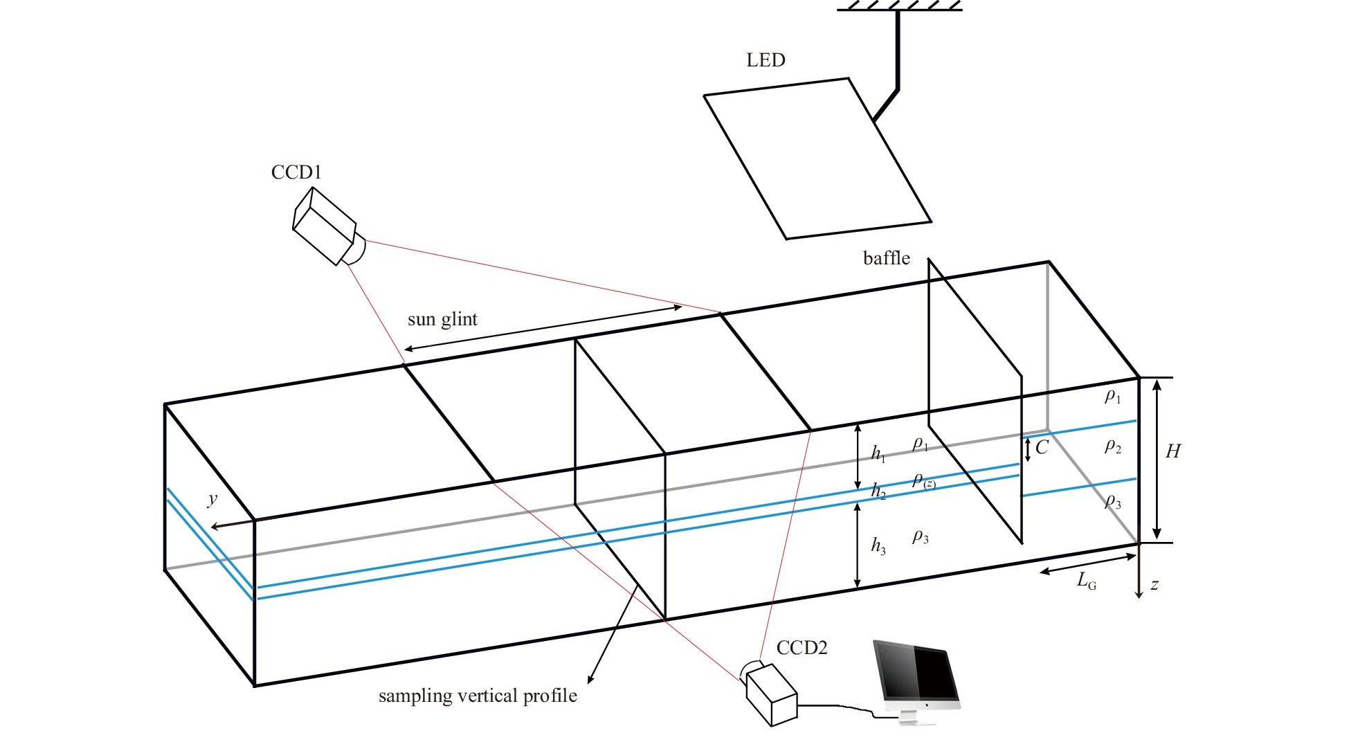
The experiment was carried out in an internal wave tank with a length of 5.0 m, a width of 0.35 m, and a height of 0.8 m (Fig. 1), with a total fluid depth of H. Within the established experimental Cartesian coordinate system (x, y, z), the y and z directions denote, respectively, the horizontal direction of wave propagation and the vertical direction parallel to the gravitational acceleration vector g = (0, 0, −g), the origin coinciding with the water surface.

Figure  1.  A schematic diagram of the laboratory experiment designed to generate mode-2 internal solitary waves (ISWs) and detect them using optical remote sensing. See the text for an explanation of all parameters. CCD: charge-coupled device; LED: Light Emitting Diode.

DownLoad: Full-Size Img PowerPoint

The stratification in the tank consisted of two layers of miscible homogeneous fluid with densities of ρ₁ and ρ₃, respectively. Before the experiment began, the prepared solution of the brine of density ρ₃ (typically 1 080 kg/m³) was filled into the tank as the lower layer with thickness h₃, and brine with density ρ₁ (typically 1 000 kg/m³) was slowly added into the tank as the upper layer with thickness h₁. Filling was achieved using a floating sponge. During the adding of the upper layer, a pycnocline with an initial thickness of h₂ and density of ρ_(z) linearly varying with depth was formed at the interface between the upper and lower layers, and h = h₂/2 as the characteristic thickness of the interface, is used to normalize the measured length scales (Salloum et al., 2012; Maxworthy, 1980). After each experiment, the characteristic thickness of the interface will change. Therefore, before each experiment, it needs to be pre-photographed by the charge-coupled device (CCD) camera and measured by the pixel extraction method. In all experiments, h was controlled within a narrow range (0.015≤h/H≤0.039).

An ISW was generated by the gravitational collapse of a layered fluid (Honji et al., 1995; Wu, 1969; Carr et al., 2019). A baffle was inserted at a distance L_G (Fig. 1) away from the end wall on the right side of the water tank until the bottom of the baffle was below the pycnocline but ensuring some space between the baffle and the bottom of the water tank.

The density of the upper layer and the lower layer in the collapse area were ρ₁ and ρ₃, respectively. The density of the middle layer was ρ₂= (ρ₁+ρ₃)/2. The initial step depth C was defined as the height difference between the upper interface of the middle layer in the collapse area and the upper interface of the pycnocline in the experimental area. The baffle was pulled out quickly and smoothly, and the mixed fluid intruded along the interface, forming a mode-2 ISW propagating to the left at the interface. The initial water surface was smooth and level. In total, 26 experiments were implemented by changing the height of the stratification and the initial step depth. Table 1 shows the parameter settings for each experiment.

Table  1.  Experimental parameters for the 26 individual experiments performed in the study

No.	H/cm	h1/H	h/H	C/h
1	40	0.475	0.028	5.33
2	40	0.475	0.031	6.43
3	40	0.375	0.014	8.85
4	40	0.375	0.024	5.24
5	40	0.375	0.031	5.69
6	40	0.338	0.015	8.20
7	40	0.338	0.037	3.39
8	40	0.338	0.041	4.26
9	40	0.313	0.021	8.33
10	40	0.313	0.039	3.19
11	40	0.288	0.025	6.97
12	40	0.288	0.029	4.29
13	40	0.288	0.039	3.22
14	40	0.263	0.026	6.73
15	40	0.238	0.026	6.73
16	40	0.238	0.039	3.19
17	40	0.213	0.024	7.33
18	40	0.213	0.028	4.48
19	46	0.417	0.017	9.21
20	46	0.417	0.038	5.75
21	46	0.370	0.021	7.18
22	46	0.370	0.038	5.71
23	46	0.315	0.024	4.57
24	46	0.315	0.034	4.52
25	46	0.261	0.018	5.92
26	46	0.261	0.029	5.17
Note: H: total fluid depth; h1: upper layer thickness; h: characteristic thickness of the interface; C: initial step depth.

 | Show Table

DownLoad: CSV

2.2 Data collection

As shown in Fig. 1, a Lighting Emitting Diode surface light source with uniform radiation was placed on the right side of the tank, and the quasi-parallel beam emitted was used to represent sunlight incident to the sea surface. Camera CCD1 was placed above the left side of the water tank to simulate an optical remote sensing sensor and to obtain optical remote sensing images of the experimental ISWs. Camera CCD2 faced the side of the water tank and was level with the height of the pycnocline to obtain the waveform of the generated ISW. To achieve synchronous acquisition of optical remote sensing images and the waveform of the generated ISW, we calibrated the fields of view of the two CCD cameras to ensure that their field of view and sampling location were consistent, the red dotted line in Fig. 1 represents the field of view of the two CCD cameras. The two CCD cameras are unified and controlled by a computer to acquire images simultaneously at a sampling rate of 35 frames per second.

A suitable sampling vertical profile was selected in the sun glint of the camera CCD1 (Fig. 1). Camera CCD1 sampled along the horizontal top edge of this section. Camera CCD2 sampled along the vertical edge of this section. Time series processing was carried out on the images obtained. Changes in pixel values of a given column with time can be obtained from the images recorded by the CCD cameras, so that the waveform of the generated ISW could be obtained from camera CCD2 (Fig. 2a), and the optical remote sensing image (Fig. 2b) obtained from camera CCD1. By making a line perpendicular to the wavefront and in the opposite direction to the wave propagation in the optical remote sensing image, the corresponding profile curve of gray value can be obtained (Fig. 2c), the y-axis is the absolute gray value, which is defined as the difference between the profile curve of gray value and the initial background. The bright-dark order of the stripes can be clearly analyzed from the curve.

Figure  2.  An example time series diagram from Experiment 1. a. Waveforms of the internal solitary wave (ISW) from camera CCD2; b. optical remote sensing image of the ISW from camera CCD1 (y-axis is horizontal sampling width); c. y-axis is absolute gray value.

DownLoad: Full-Size Img PowerPoint

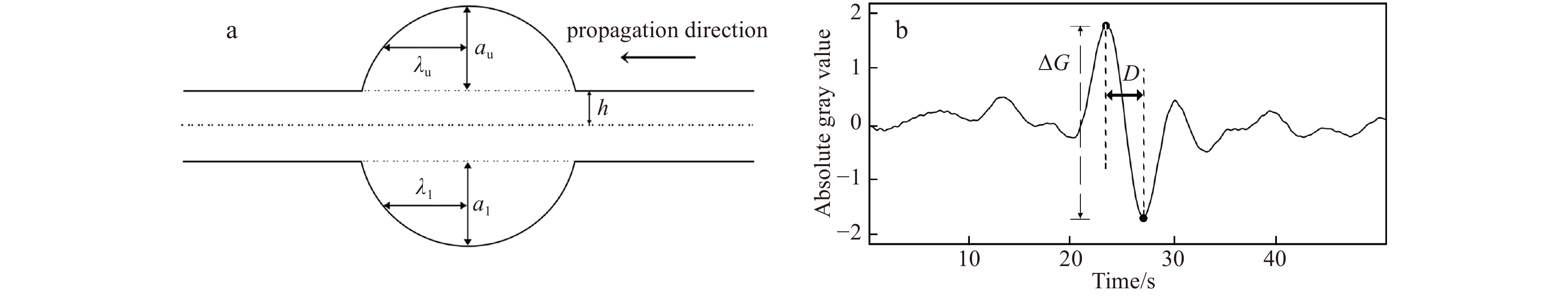
The amplitude a and wavelength $\text{λ} $ of the ISW were extracted from the waveform diagram. As illustrated by Fig. 3a, the amplitude was defined as the maximum displacement of the upper and lower isopycnals of the pycnocline, and the wavelength refers to the horizontal distance from the location where half of the amplitude was located to the peak/trough. The amplitude and wavelength of the upper and lower interfaces were a_u and a_l, $ {\text{λ} }_{{\rm{u}}} $ and $ {\text{λ}}_{{\rm{l}}} $, respectively. However, in the laboratory, the back part of a large amplitude wave often tends to lead to mixing enhancement with density stratification, therefore, the first half of the wave was used to measure the wavelength (Carr et al., 2015; Stamp and Jacka, 1995). The optical remote sensing characteristic parameters of the ISWs were extracted from the profile curve of gray value (Fig. 3b), the difference in gray value between the two peak points was defined as the gray difference ΔG, and the distance between the brightest and darkest regions of the stripe was defined as the bright-dark spacing D.

Figure  3.  Details of parameter definitions describing a mode-2 internal solitary wave (ISW). a. Wave parameters of the mode-2 ISW; b. optical remote sensing characteristic parameters of the mode-2 ISW.

DownLoad: Full-Size Img PowerPoint

3. Results and discussion

3.1 Correspondence between laboratory and in situ optical remote sensing imagery

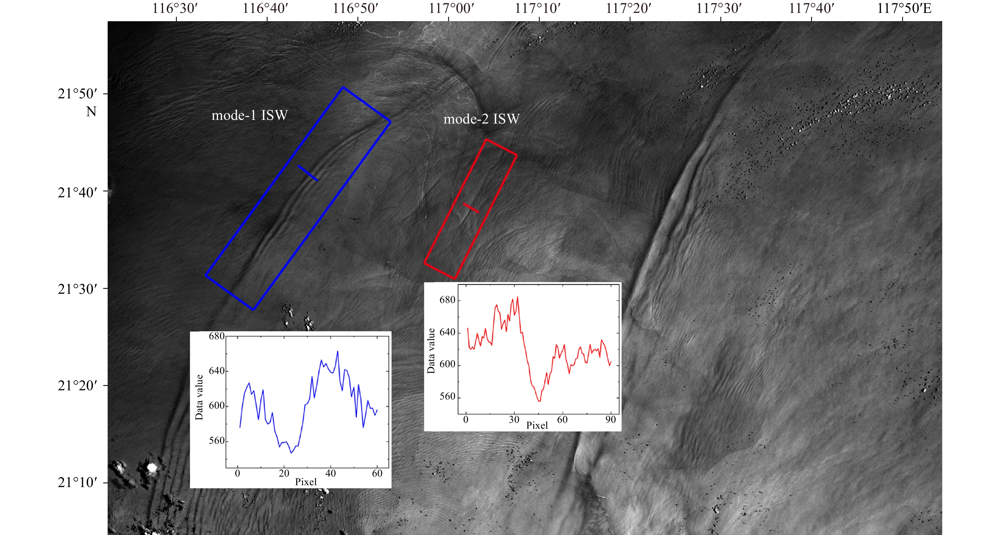
Within the sun glint of optical remote sensing images, the stripes of mode-1 ISWs are exactly opposite to those of convex mode-2 ISWs when the upper layer in the ocean is thinner than the lower layer (Hennings et al., 1994; Melsheimer and Kwoh, 2001; Yang et al., 2010; Huang et al., 2012), and the imaging features are reversed when outside the sun glint (Jackson and Alpers, 2010). Figure 4 shows a Gaofen-1 optical remote sensing image obtained north of Dongsha Islands taken on July 9, 2014. The figure clearly shows that the ISWs propagate from southeast to northwest within the sun glint. From the profile curve of gray value perpendicular to the wave front and opposite to the direction of wave propagation given in Fig. 4, the stripes of the mode-1 ISWs in the blue box show the dark-bright order, and in the red box are just the opposite. The temperature and salinity data provided by World Ocean Atlas 2018 (WOA18) were used to determine the water depth and stratification at the location of the red box, which is consistent with the hydrological conditions for the presence of convex mode-2 ISWs, and based on the observations of Yang et al. (2009) in the northern South China Sea, 90% of mode-2 ISWs follow the propagation of mode-1 ISWs in summer. Therefore, it can be judged that the red box highlights the convex mode-2 ISWs.

Figure  4.  Gaofen-1 image taken north of Dongsha Islands on July 9, 2014. The blue box highlights a mode-1 internal solitary wave (ISW), and the red box highlights a mode-2 ISW. Profile data for the two ISWs are given in the insert figures. The mode-1 ISW shows dark-bright stripes, while the mode-2 ISW is the opposite.

DownLoad: Full-Size Img PowerPoint

From Fig. 2, we have seen that an ISW in the experimental tank presents stripes in bright-dark order in the optical remote sensing image. The optical remote sensing images of the mode-2 ISWs obtained in our laboratory experiments have similar characteristics as those detected by ocean optical remote sensing, confirming that the experimental platform can effectively simulate optical remote sensing imaging of mode-2 ISWs in the ocean.

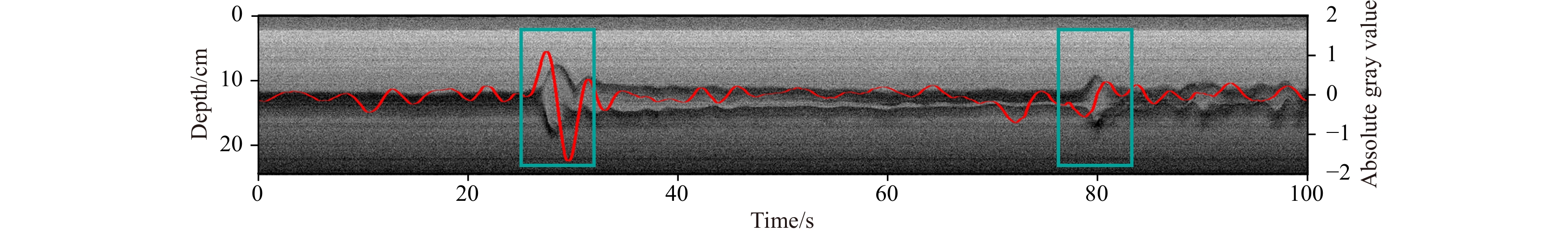
To verify the corresponding relationship between the imaging location and time of the optical remote sensing image and the waveform in the experiment, the profile curve of gray value was superimposed with the generated waveform for comparison. An example is presented in Fig. 5. Here, 3500 images taken during Experiment 12 are used for time series processing. In the figure, the wave sampled 25 s to 35 s after the start of the experiment was the initial wave propagating from right to left in the tank, past the sampling line. The wave sampled about 80 s had elapsed was the wave that had propagated to the end face of the water tank and had been reflected to the sampling line. The extreme values of the profile curve of gray value represent the brightest/darkest locations in the stripes of the optical remote sensing image.

Figure  5.  Example diagram showing the matching of internal solitary wave (ISW) properties and profile curve of gray value of the associated remote sensing image. This time series was obtained from Experiment 12 (i.e., h₁/H=0.288, C/H=4.29; the definitions of h₁, H, C refer to Fig. 1). The left vertical axis represents the vertical sampling range in the tank, the right vertical axis represents the absolute gray value, and the horizontal axis represents the charge-coupled device camera shooting time. The blue boxes at the sampling time of about 30 s and 80 s represent the initial wave and reflected wave at the sampling location, respectively. The red curve is the profile curve of gray value recorded at the sampling location.

DownLoad: Full-Size Img PowerPoint

Comparing the locations of the extreme values in the profile curve with the waveform, it can be seen that the extreme points are in good agreement with the upper and lower interfaces of the ISWs: i.e., the extreme value points appear near the half-waist of the mode-2 ISWs. This conforms to the modulation theory of ISWs in the ocean (Alpers, 1985; Zheng et al., 2001). The coincidence of the wave features with the variation of the gray values confirms that the spatiotemporal positioning of the images obtained by the two CCD cameras is aligned.

In conclusion, the optical remote sensing simulation experiment in this paper can effectively simulate in situ optical remote sensing imaging of ISWs in the actual ocean. The laboratory setup solves the problem of space-time matching between the image and the field-measured data in the process of parameter inversion of ISWs based on optical remote sensing imagery. At the same time, it allows us to study the correlation between optical remote sensing characteristic parameters and wave parameters.

3.2 Characteristics of mode-2 ISWs with large amplitudes

Understanding the characteristics of ISWs is helpful for us when studying the relationship between wave parameters and lays a foundation for later analysis (Stamp and Jacka, 1995). The characteristics of large amplitude mode-2 ISWs were studied using 26 sets of experiments covering different initial step depths and hydrological conditions, and the amplitude of the ISWs was in the range of 2.1<a/h<7.3.

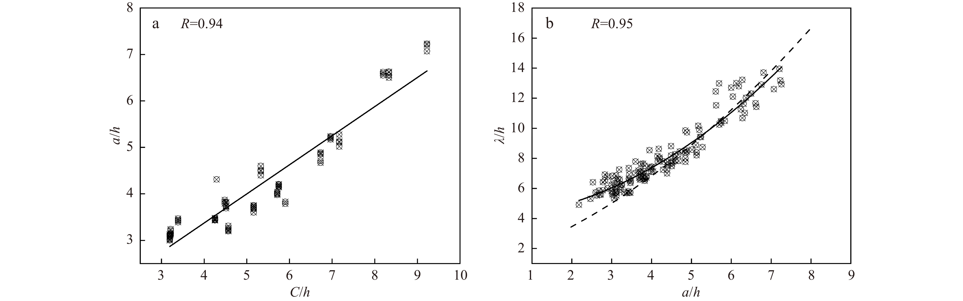
Figure 6a describes the influence of initial step depth on the average amplitude of an ISW (i.e., a=(a_u+a_l)/2) and shows that the average amplitude increased linearly with initial step depth. The solid line shows the results of a least-squares linear fit, and the linear correlation coefficient was R=0.94, indicating that the amplitude can be kept roughly constant at the same initial step depth. This lays the foundation for subsequent data analysis.

Figure  6.  Wave parameter relationship diagrams for mode-2 internal solitary waves (ISWs). a. Relationship between average amplitude and initial step depth; b. relationship between average amplitude and average wavelength. The data points are the experimental data in this paper, and the solid black lines are the fitting of the experimental data. The black dotted lines are the experimental results of Brandt and Shipley (2014).

DownLoad: Full-Size Img PowerPoint

The ISW wavelength as a function of wave amplitude is shown in Fig. 6b, fitted by least squares with a correlation coefficient of R=0.95, and the experimental results of Brandt and Shipley (2014) are also included. From the fitting line, it can be found that when a/h<4, the data extracted by Brandt and Shipley (2014) are small. The data extraction method may be the main reason for this phenomenon, we extract the amplitude by calculating the maximum displacement of the isopycnals, while Brandt and Shipley (2014) used a dye to extract the amplitude and wavelength based on the bulge characteristics inside streamlines. The internal bulge of the small amplitude wave itself has a more compact nature, so the extracted data will be smaller. As the amplitude continues to increase, our experimental data agree better with the results of Brandt and Shipley (2014) with an increase in wavelength for large amplitude ISW. At a/h≈4, the linear form was obviously broken, and the nonlinear relationship became stronger with increasing amplitude, which also suggests that the dependence of the wavelength on the higher-order terms of amplitude is more obvious for large amplitudes. Brandt and Shipley (2014) also mentioned in their research that the convex characteristics of ISWs will make their shape narrow and long with increasing amplitude. This further confirms the nonlinear relationship between amplitude and wavelength under large amplitude.

3.3 Correlation between bright-dark spacing and wavelength

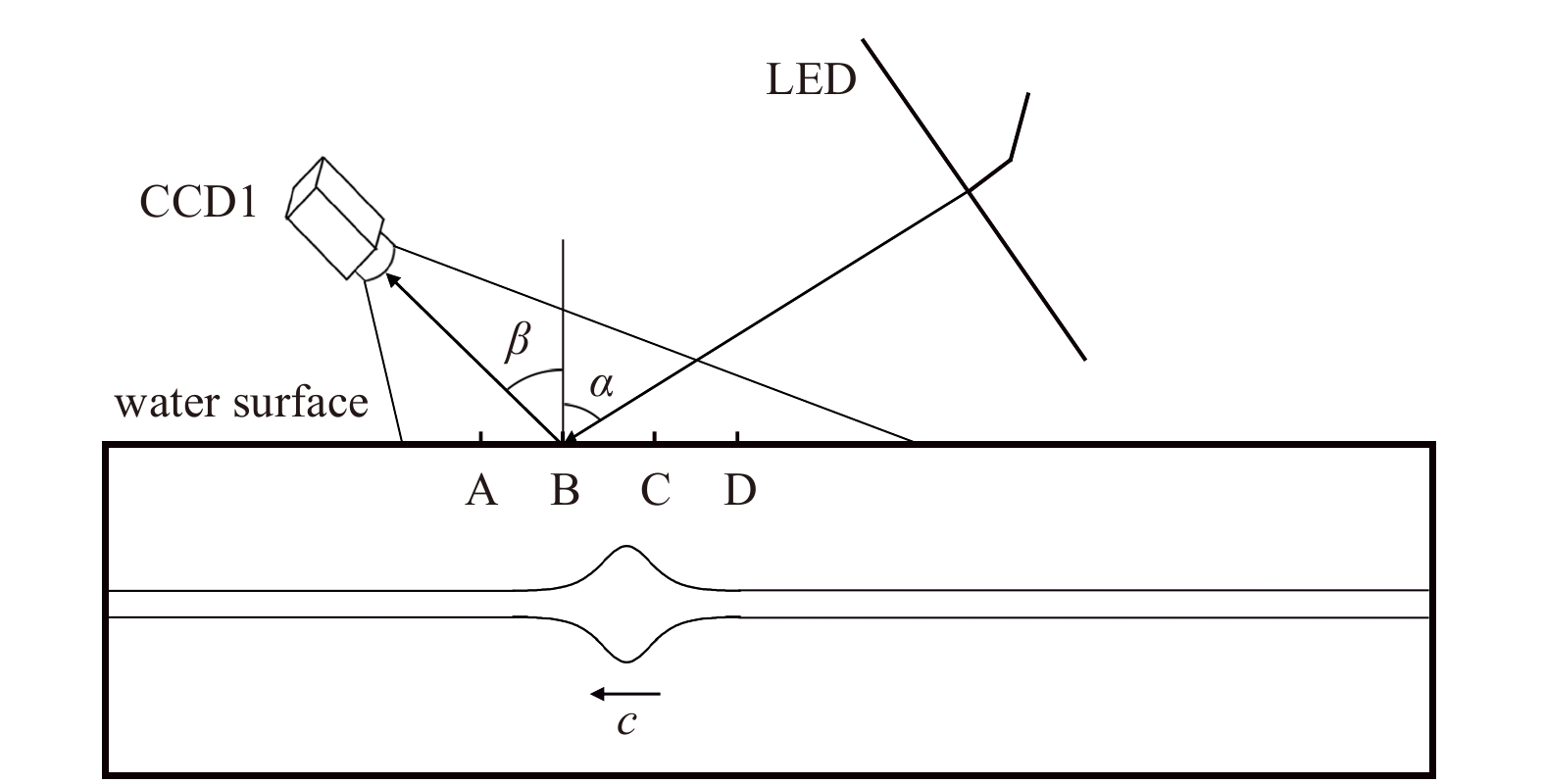
As a characteristic parameter in optical remote sensing imagery, bright-dark spacing plays an important role in the parameter inversion of mode-1 ISWs (Wang et al., 2021). Zheng et al. (2001) proposed a peak-to-peak method based on SAR images, which uses the bright-dark spacing to invert the characteristic half width of mode-1 ISWs and thus calculate the amplitudes. Similarly, in the current experimental study of mode-2 ISWs, we need to explore whether there is a correlation between the bright-dark spacing and the wavelength and hope to get a quantitative relationship between them. Therefore, we selected four different imaging locations in the sun glint (Fig. 7, A to D), and by time series processing of the sampled profiles at these four locations, we were able to extract the bright-dark spacing and wavelength of the initial incident waves in the experiment. The zenith angle is the angle between the zenith line (pointing straight up) and the direction of the sun (sensor).

Figure  7.  Schematic diagram of sampling location and imaging angle. A−D are all in the sun glint. Initial incident wave propagation from right to left. $ \mathrm{\alpha } $ is the solar zenith angle, and $ \ {\beta } $ is the sensor zenith angle. LED: Light Emitting Diode; CCD: charge-coupled device.

DownLoad: Full-Size Img PowerPoint

To exclude the interference of other factors, we first investigated the relationship between the bright-dark spacing and wavelength at the same imaging location. Figure 8 shows our least-squares linear fit of the data at location A for several sets of eligible experiments. It is obvious that the bright-dark spacing of mode-2 ISW shows a positive correlation with wavelength similar to that of mode-1 ISW, and the relationship between wavelength and bright-dark spacing at the lower interface is better than that at the upper interface, and the correlation between the average wavelength and bright-dark spacing is the best, with the corresponding correlation coefficients are R_u=0.88, R_l=0.91, and R_a=0.95, respectively.

Figure  8.  Bright-dark spacing versus wavelength in internal solitary wave optical remote sensing images. a. The relationship between the bright-dark spacing and the wavelength of the upper interface; b. the relationship between the bright-dark spacing and the wavelength of the lower interface; c. the relationship between the bright-dark spacing and the average wavelength.

DownLoad: Full-Size Img PowerPoint

Using the same method, we extracted and analyzed the data and correlation coefficients of the other three locations, as shown in Table 2, the correlation between the wavelengths of the lower interface and the bright-dark spacing of these locations is almost all better than that of the upper interface, and the correlation between the average wavelength and the bright-dark spacing is the best. The reason for this phenomenon has not been determined and it may be caused by the K-H type instability of large amplitude mode-2 ISWs or by the asymmetry of the upper and lower interfaces due to the offset pycnocline, but it is worth being sure that the imaging of mode-2 ISWs in optical remote sensing images is produced by the overall modulation effect of ISWs on the water surface.

Table  2.  Correlation coefficients between bright-dark spacing and wavelength at a series of locations along the tank

Location	Solar zenith angle	Sensor zenith angle	Ru	Rl	Ra
A	55.8°	51.3°	0.88	0.91	0.95
B	55.2°	53.3°	0.88	0.89	0.92
C	54.4°	55.5°	0.92	0.88	0.92
D	53.7°	57.5°	0.81	0.86	0.87

 | Show Table

DownLoad: CSV

From Table 2, we can see that with the sampling location from A to D, the change of the sensor zenith angle was greater than that of the solar zenith angle. Comparing the fitting results of wavelength and bright-dark spacing at four locations, as shown in Fig. 9, the slope of the best fitting line decreased with the decrease of the solar zenith angle and the increase of the sensor zenith angle, and the overall change is not significant, indicating that the extraction of the bright-dark spacing in the experiment is little affected by the imaging angle, so we can analyze the data from several sampling locations in a comprehensive manner, and the black solid line in Fig. 9 is the result of fitting with all the data from the four sampling locations of A−D. The linear correlation coefficient R=0.91 and the non-dimensional relationship between bright-dark spacing and wavelength can be described as

which indicates that there is a strong correlation between the wavelength of mode-2 ISW and its bright-dark spacing in optical remote sensing images, and lays the foundation for the parameter inversion of mode-2 ISW based on optical remote sensing images.

Figure  9.  Relationship between bright-dark spacing and wavelength at different angles. The least-square fitting results of four sampling locations A (blue dotted line), B (red dotted line), C (orange dotted line), and D (green dotted line), and the fitting results of all data (black solid line) are presented.

DownLoad: Full-Size Img PowerPoint

3.4 Correlation between bright-dark spacing and amplitude

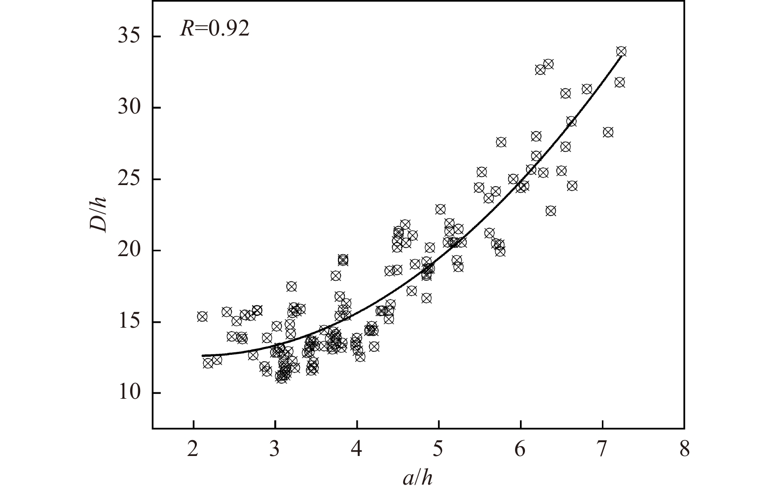
The bright-dark spacing and the average amplitude of ISWs under all experimental conditions in Table 1 were fitted to obtain the curves shown in Fig. 10, and the nonlinear relationship was described as

The fitting correlation coefficient between bright-dark spacing and the average amplitude is 0.92, which indicates a good correlation. When 2.1<a/h<4, the bright-dark spacing changes slowly with the increase of amplitude. When 4<a/h<7.3, the bright-dark spacing increases significantly with increasing amplitude, showing a nonlinear relationship over the entire range. According to the experimental study of Brandt and Shipley (2014), VLISW has a more eccentric shape, and its strong internal recirculation may be the reason for the unusually large growth rate of wavelength, the nonlinearity of the scaling of the wavelength with amplitude became apparent and more obvious dependence on the second order term, which subsequently leads to a nonlinear relationship between the bright-dark spacing and amplitude. For this reason, the relationship between bright-dark spacing and wavelength and amplitude given in this paper is only applicable to the amplitude range used in this experiment.

Figure  10.  Fitting curve of bright-dark spacing with amplitude.

DownLoad: Full-Size Img PowerPoint

Through the preliminary study of the bright-dark spacing seen in optical remote sensing images and the wave parameters of mode-2 ISWs, it can be concluded that there are correlations between amplitude, wavelength, and bright-dark spacing, which provides the possibility of inverting amplitude by using the bright-dark spacing of mode-2 ISWs in optical remote sensing images and lays the foundation for further research.

4. Conclusions

The inversion of the wave parameters of mode-2 ISW based on optical remote sensing images is a pressing issue. In this paper, the relationship between optical remote sensing imaging characteristics and wave parameters of a large amplitude convex mode-2 ISW is investigated using a laboratory-based optical remote sensing simulation platform, which provides an experimental basis for parameter inversion of mode-2 ISW based on optical remote sensing images. In the experiment, a series of convex mode-2 ISWs are generated by setting different water stratification structures and initial step depths, and the optical remote sensing images and waveforms of the ISWs are obtained synchronously by two CCD cameras. The bright-dark stripes of mode-2 ISWs in the experiment are consistent with those seen in the ocean, which confirms that the optical remote sensing simulation experiment designed in this paper can effectively simulate the optical remote sensing imaging of ISWs in the actual ocean, thus helping to solve the problem of space-time matching between images and field-measured data.

The characteristics of ISWs with 2.1<a/h<7.3 are analyzed. The results show that the wavelength of large amplitude ISWs increases with increasing amplitude, and the linear form is broken at a/h≈4. When a/h>4, the nonlinear effect of wavelength with amplitude increases, suggesting a second-order dependence of wavelength on amplitude in the case of large amplitudes.

In addition, the following relationships between optical remote sensing characteristic parameters and the wave parameters of ISW were observed:

(1) By comparing the correlation between the bright-dark spacing and the wavelength of different interfaces, it was seen that the optical remote sensing images are produced by the overall modulation effect of the ISWs on the water surface. A non-dimensional correlation between the bright-dark spacing and the wavelength was obtained by using the least-square method, and the influence of the imaging angle on the correlation between the two was explored. This lays a foundation for the parameter inversion of mode-2 ISWs based on optical remote sensing imagery.

(2) The correlation between bright-dark spacing and wave amplitude was studied using experimental data. The results show that there is a nonlinear relationship between the two, especially at very large amplitudes. Compared with ISW with a smaller amplitude, VLISW has a more eccentric shape, and its strong internal recirculation may be the reason for the apparent nonlinearity of the bright-dark spacing in the variation with amplitude. The nonlinear relationship between the two also offers the possibility to invert the amplitude of mode-2 ISW directly using the bright-dark spacing in optical remote sensing images in the future.

Different from the general mode-1 ISWs, mode-2 ISWs have strong regions of internal recirculation, which affects the mixing process of the upper ocean and is worth further studying. The more refined hydrological conditions are of great importance in the subsequent work for further extension to the ocean.