A case study of continental shelf waves in the northwestern South China Sea induced by winter storms in 2021

1. Introduction

Continental shelf waves (CSWs) are typical sub-inertial motions resulting from the conservation of potential vorticity on the continental shelf. On an f-plane, the displacement of water columns across bottom topography creates positive and negative relative vorticity (Weber and Drivdal, 2012). The waves result from the conservation of vorticity are trapped over the continental shelf, propagating along the shelf with the coast on their right in the northern (southern) hemisphere (Pedlosky, 1987). The phase speed of CSWs depends on the bottom topography, ranging from one to tens meters per second (Schulz et al., 2012). And the period of CSW reported in previous research ranges from 2 d to 30 d (Chen and Su, 1987; Li, 1993; Wang et al., 2021). This kind of waves combined with deep eddy signals could explain approximately 60% of the kinetic energy of the currents (Shu et al., 2022). The propagation of CSW could dynamically modulate coastal current through the sea level-related barotropic pressure gradient, leading to an important influence on coastal circulation and ecosystem (Ding et al., 2012; Lin and Yang, 2011; Lin et al., 2011).

The northern South China Sea (SCS) is characterized by a broad continental shelf with a width of ~200 km from the coast to the area with a depth >200 m as shown in Fig. 1, which provides a favorable condition for the generation and propagation of CSWs. Moreover, typhoons and winter storms are the major atmospheric processes for the generation of CSW in the northern SCS (NSCS). Previous studies of ocean response to typhoon and winter storm have focused on the generation and propagation of CSWs along the northern coast of the SCS (Chen and Su, 1987; Ding et al., 2012; Li et al., 2015; Li, 1993; Shen et al., 2017, 2021; Shu et al., 2016; Zhao et al., 2017; Zheng et al., 2015). The signals with periods ranging from 2 d to 10 d occur in the tidal gauge data (Li, 1993). The phase speed of CSW is about 5–18 m/s varying with the depth of shelf profile (Ding et al., 2012; Li et al., 2015; Shen et al., 2021). Zheng et al. (2015) investigated a resonant effect on CSW generation induced by a moving storm over the continental shelf. The typhoons produce episodic forcing on the sea water and provide enough power supplies for the growth and evolution of CSW (Li et al., 2021). Ding et al. (2012) found that mode 2 CSWs are induced by typhoon in a stratified ocean in summer using a three-dimensional numerical model. In winter, the signals of sea level oscillation are closely associated with northeasterly wind burst (Huang et al., 2016).

Figure  1.  Study area and locations of observation stations. Blue dots are locations of tidal gauge stations of Hong Kong (HK), Zhapo (ZP) and Qinglan (QL). Red square is the location of mooring station MO. Red dots represent cruise observation section SE. Black lines represent sea surface wind observation sections W1, W2, W3 and W4. Coordinate system x-o-y is set as x-axis perpendicular to the coastline seaward positive and y-axis parallel to the coastline leftward positive. θ (= 35°) is the y-axis direction referring to true north. Contours display water depth.

DownLoad: Full-Size Img PowerPoint

In addition to the Coriolis effect and bottom topography, remote forcing is also important for CSW generation (Li et al., 2015). Jacobs et al. (1998) found that the Kelvin mode of CSW transmits the sea surface height signals and the potential energy anomaly southward from the East China Sea (ECS). Yin et al. (2014) also found that the sea level variation mainly results from the Kelvin mode of CSW in the ECS. Ding et al. (2012) concluded that the remote forcing dominates the positive wave signals in the model results, whereas the local wind forcing dominates the negative signals over the SCS shelf.

The northwestern SCS adjoins the wide continental shelf in the east and connects the Beibu Gulf through the Qiongzhou Strait in the west. On the south side, there is a SCS deep basin with a maximum depth reaching 5000 m. On the northeast side, the Zhujiang River (Pearl River), the third largest river in China, inputs fresh water onto the shelf as high as 3.492 × 10¹¹ m³ per year, which is partially transported to the study area by the westward Guangdong Coastal Current during the northeasterly (winter) monsoon. In winter, the atmospheric circulation is featured by prevailing northeasterly winds, and winter storms pass over the area every 3–10 d (Chen and Su, 1987). The sea level over the continental shelf presents as a kind of arrested topographic wave influenced by the prevailing wind forcing (Lin et al., 2022).

Chen and Su (1987) found that the phase speed of CSW between Hong Kong (HK) and Zhapo (ZP) reaches 17 m/s, which is much higher than 6–8 m/s in the northern SCS in winter. Li (1993) suggested that the fast waves near station HK should be standing waves. The mechanism is attributed to distinct stratification conditions, i.e., the water is strong stratified on the west side of the shelf, but well mixed near the Pearl River Estuary on the east side of the shelf. This scenario, however, needs to be confirmed by further observations.

At this point the nature and the characteristics of the CSWs in the NSCS in winter remain to be determined. The analysis of current structure of CSW in the northern SCS from observations has not been carried out before. In this study, cruise and mooring observations and tidal gauge data in winter 2020–2021 are analyzed to examine the characteristics and controlling factors of CSWs on the continental shelf of the northwestern SCS. The rest of the paper is organized as follows: Section 2 describes the observed dataset and the analysis methods. Section 3 presents the characteristics of the CSW derived from the observed sea level fluctuations. Section 4 analyzes the relationship between CSW and the signals in along-shelf wind, and the baroclinic oceanic response. Section 5 gives a summary and conclusions.

2. Data and methods

2.1 De-tided sea level anomaly (DSLA)

Tidal gauge data at stations HK, ZP and Qinglan (QL) as shown in Fig. 1 are obtained from the Sea Level Station Monitoring Facility. The data cover a period ranging from January 1 to February 28, 2021 with a temporal resolution of 1 min. After resampling the data and removing a mean sea level, the temporal resolution of the tidal gauge data is reduced to 1 h. De-tided sea level anomaly (DSLA, as shown in Fig. 2) is obtained from the tidal gauge data by using a de-tiding software (Pawlowicz et al., 2002). The missing data occur in the tidal gauge data from ZP and QL. The linear interpolation has been applied to the missing data.

Figure  2.  Time series DSLA data at tidal gauge stations: a. HK, b. ZP, c. MO and d. QL.

DownLoad: Full-Size Img PowerPoint

2.2 Mooring data and cruise data

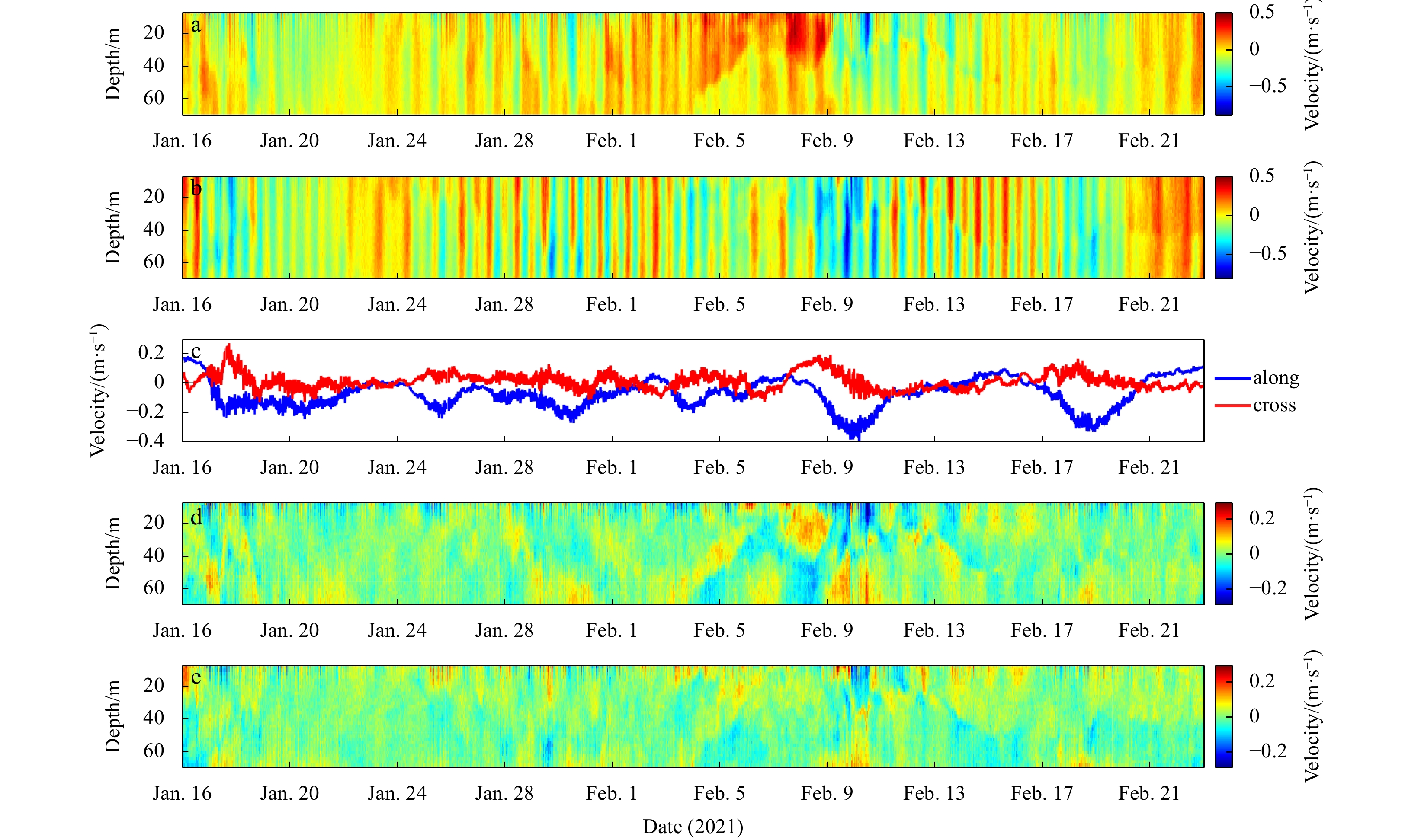
An upward-looking 300-kHz Acoustic Doppler Current Profiler (ADCP) was deployed in the northwestern SCS at the bottom depth of 70 m (shown as MO in Fig. 1) to collect the current velocity data in the upper 70 m. The sampling interval and vertical bin size were set to 10 min and 2 m, respectively. The data cover a period from January 16 to February 22, 2021.

The north and east current components are processed to along-shelf and cross-shelf components by Eq. (1).

where the subscript indicates the velocity component. Coordinate system x-o-y is set as in Fig. 1, i.e., x-axis perpendicular to the coastline seaward positive and y-axis parallel to the coastline leftward positive. θ (= 35°) is the y-axis direction referring to true north.

The barotropic and baroclinic current components (as shown in Fig. 3) are calculated from along-shelf and cross-shelf velocity components by Eq. (2).

Figure  3.  Velocity components derived from mooring observed data. a. Cross-shelf current component, b. along-shelf current component, c. barotropic current component, d. baroclinic cross-shelf current component and e. baroclinic along-shelf current component.

DownLoad: Full-Size Img PowerPoint

where U_b and U_c are the barotropic and baroclinic velocity, respectively.

The barotropic and baroclinic velocity components are calculated as

where m is bin number in vertical direction of the data.

The signal amplitudes in DSLA at stations HK, ZP and QL are larger than 0.1 m, thus, we use the DSLA derived from the pressure sensor deployed on ADCP (shown in Fig. 2c) as an auxiliary data for the analysis of sea level signals.

Cruise section measurements (red dots as shown in Fig. 1) were carried out on January 15, 2021. The temperature, salinity profiles were collected using a Sea-Bird 911plus conductivity-temperature-depth (CTD) system. The buoyancy frequency $ N=\sqrt{\dfrac{g}{\rho_{\mathrm{w}} }\dfrac{\partial \rho_{\mathrm{w}} }{\partial z}} $ is calculated from temperature and salinity data as shown in Fig. 4, ρ_w is sea water density, g is the gravitational acceleration.

Figure  4.  Cruise observed salinity (a), temperature (b) and squared buoyancy frequency (c) along Section SE. Red dots in a indicates stations.

DownLoad: Full-Size Img PowerPoint

2.3 Sea surface wind

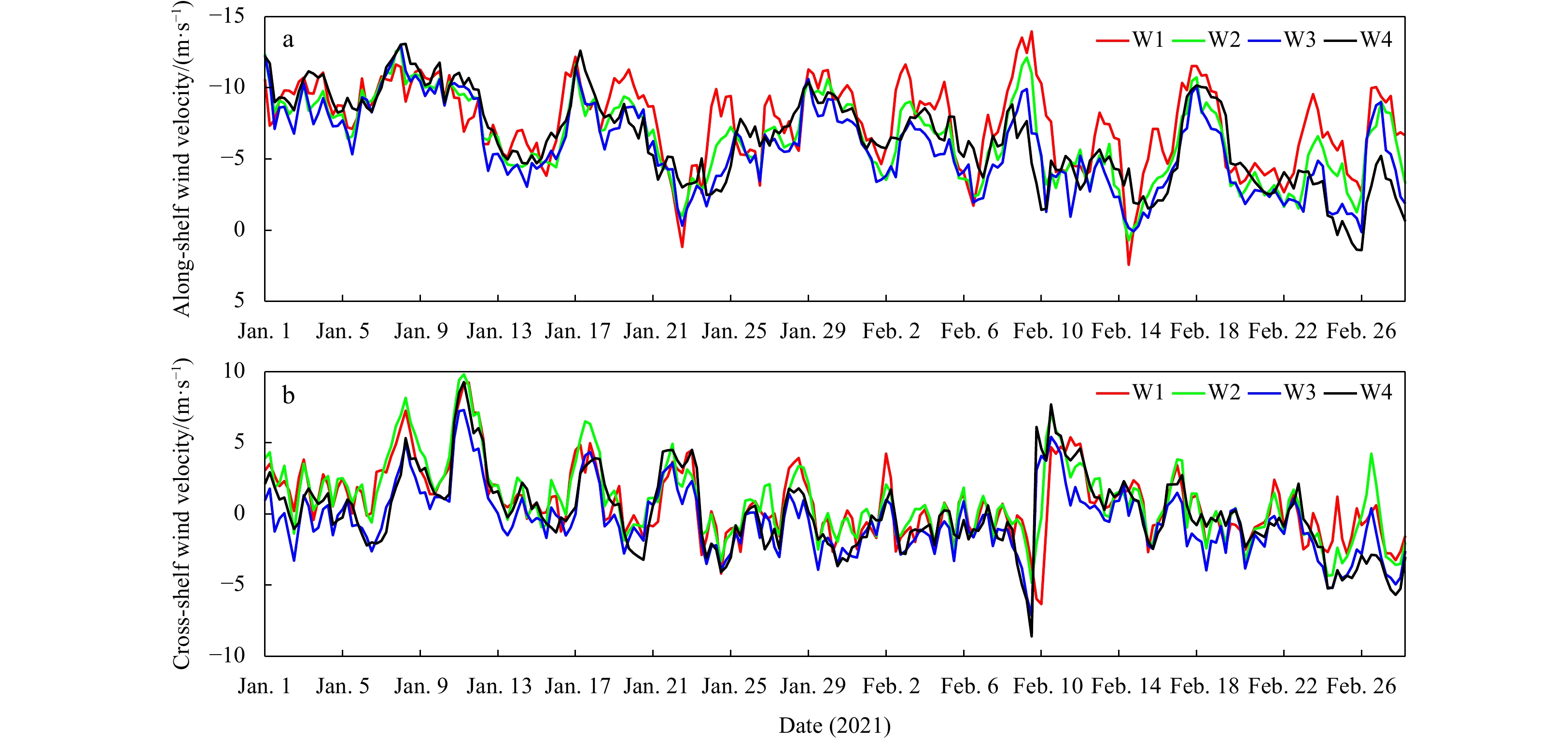
Sea surface wind data are obtained from the Copernicus Marine Environment Monitoring Service (CMEMS). The product is derived from scatterometers on board ASCAT-A and ASCAT-B. The data are calculated from Level-2b products in combination with European Centre for Medium-Range Weather Forecasts (ECMWF) operational wind analyses from January 2016. Temporal resolution of the dataset is 6 h, and spatial resolution is 0.25° × 0.25°. The data are performed for each synoptic time (00:00, 06:00, 12:00, 18:00 UTC), and cover a period from January 1 to February 28, 2021.

Sea surface wind collected on sections W1, W2, W3 and W4 (as shown in Fig. 1) are used for this study. The wind vectors are decomposed into the cross-shelf and along-shelf wind components on the continental shelf area using Eq. (1). Time series of averaged along-shelf and cross-shelf wind components on wind sections are shown in Fig. 5.

Figure  5.  Time series of sea surface wind component derived from CMEMS wind product. a. Along-shelf wind; b. cross-shelf wind at sections W1 (red curve), W2 (green curve), W3 (blue curve) and W4 (black curve).

DownLoad: Full-Size Img PowerPoint

The along-shelf wind stress is calculated by Hellerman and Rosenstein (1983) as

where ρ_a, C_D and U are the air density, drag coefficient and along-shelf wind velocity, respectively.

The drag coefficient is calculated according to the formulation recommended by Garratt (1977) as follows:

2.4 Wavelet analysis

The wavelet transform is used to analyze time series containing nonstationary power with different frequencies (Torrence and Compo, 1998). The wavelet transform of a variable x_n is defined as the convolution of x_n with the scaled and normalized wavelet:

where s is wavelet scale, $\text{δ} $t is time spacing, $\psi $ is wavelet.

Cross wavelet transform (XWT) is used to analyze the covariance of two time series X and Y (Grinsted et al., 2004). The distribution of XWT is defined as

where $ {{{\boldsymbol Z}}}_{\nu } \left(p\right) $ is the confidence level associated with the significance p. Asterisk indicates conjugation.

The phase difference between the periodic components of X and Y in XWT can be expressed as phase angle:

In this study, we used a wavelet transform toolbox developed by Grinsted et al. (2004) to analyze the power spectra and phase difference between current, DSLA, and sea surface wind data.

3. Results

3.1 Spectral characteristics of DSLA

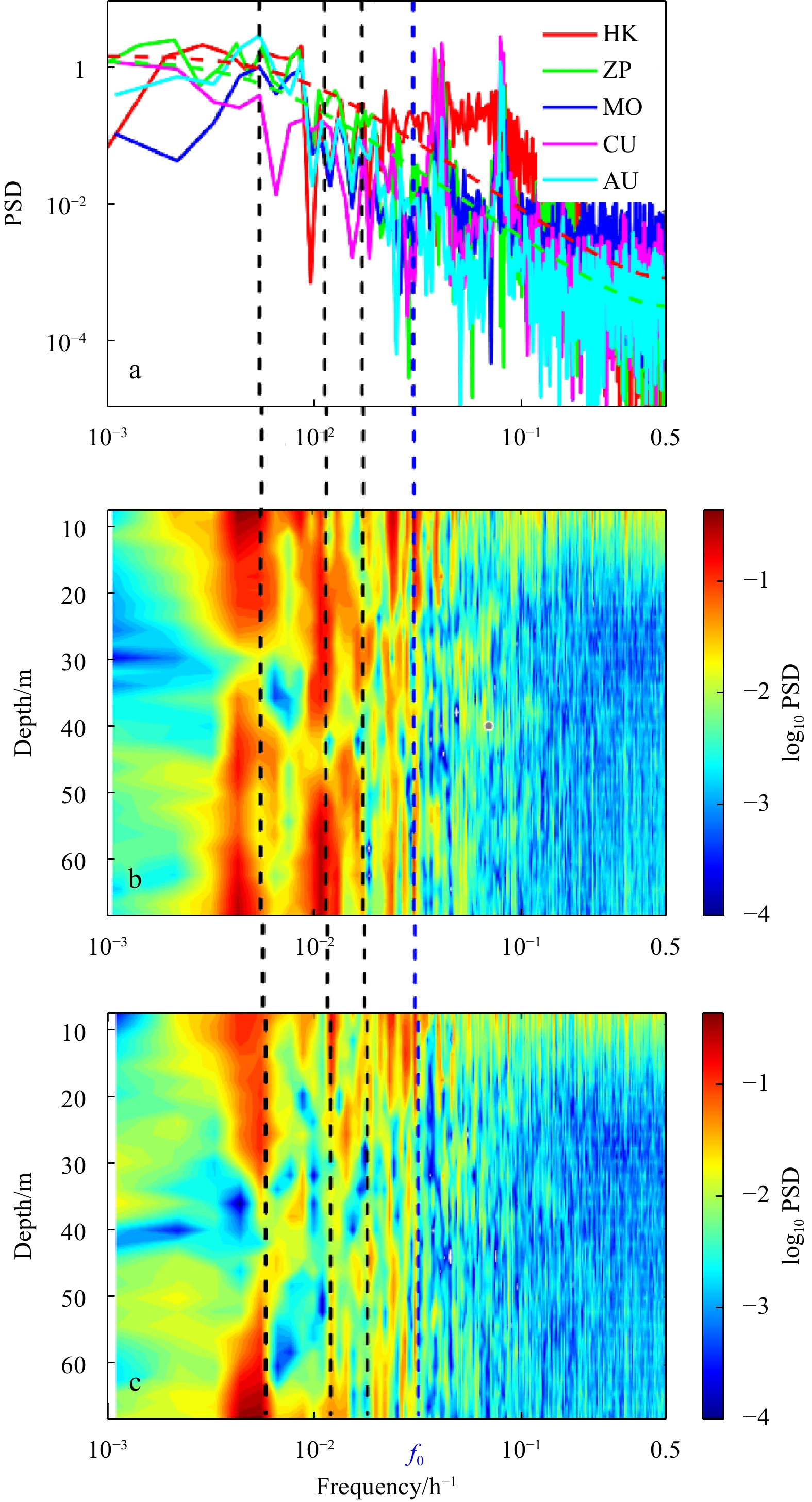
Figure 6a shows power spectral density (PSD) of DSLA at stations HK, ZP and MO. One can see that the spectra of DSLA for 3 stations are all triple peaked at frequencies of 0.0177 h⁻¹, 0.0106 h⁻¹ and 0.0056 h⁻¹ (periods of 56 h, 94 h and 180 h) in the sub-inertial band of ω < f₀ (= 0.0295 h⁻¹). The three frequency bands are also shown in the PSD of barotropic along-shelf and cross-shelf currents as well as baroclinic current.

Figure  6.  Power spectral density (PSD) of observation data. a. PSD of DSLA at stations HK (red), ZP (green), MO (blue), and that of barotropic current of cross-shelf component (CU, magenta) and along-shelf component (AU, cyan). Green and red dashed lines in a are the 5% significance level against red noise for DSLA at HK and ZP, respectively. PSD of de-tided baroclinic current of cross-shelf (b) and along-shelf components (c). Black dashed lines represent three frequency bands 0.0177 h⁻¹, 0.0106 h⁻¹ and 0.0056 h⁻¹; blue dashed line indicates the inertial frequency band (f₀).

DownLoad: Full-Size Img PowerPoint

In the vertical distribution of the PSD of baroclinic current, disconnection occurs at the depth of about 30–40 m, especially for the frequency band of 0.0056 h⁻¹. As can be seen from Fig. 4, two layers exist over the shelf. One is the mixed layer above 30 m, and the other is below the mixed layer with the depth deeper than 40 m. Therefore, the disconnection of PSD shows the stratification of the sea water (Zhang et al., 2014; Zhou et al., 2005). The result indicates that the high-order modes of the signals exist over the shelf. Meanwhile, the PSD of the cross-shelf baroclinic current component is much larger than that of along-shelf baroclinic current component. Thus, it is reasonable to conclude that the three frequency bands are dominant energy-containing bands of the sub-inertial signals in the study area.

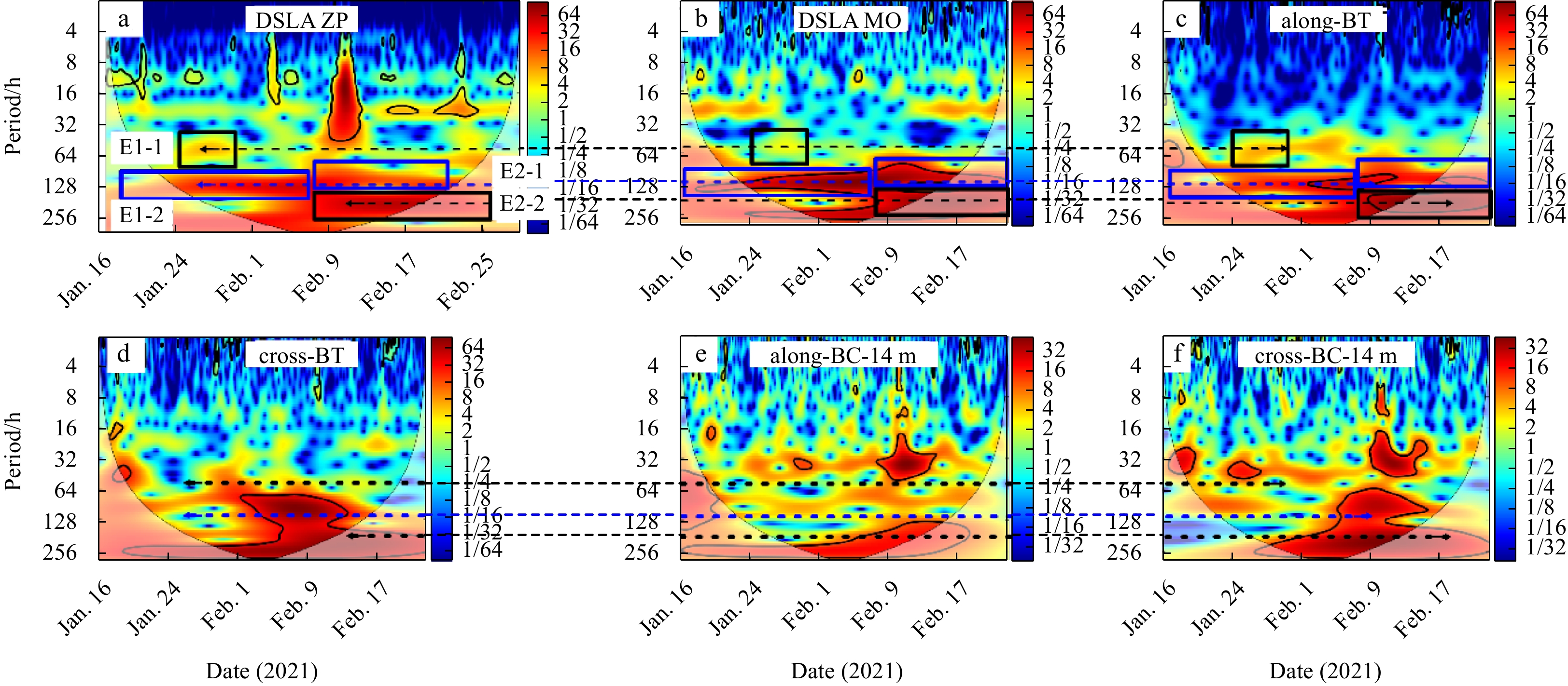
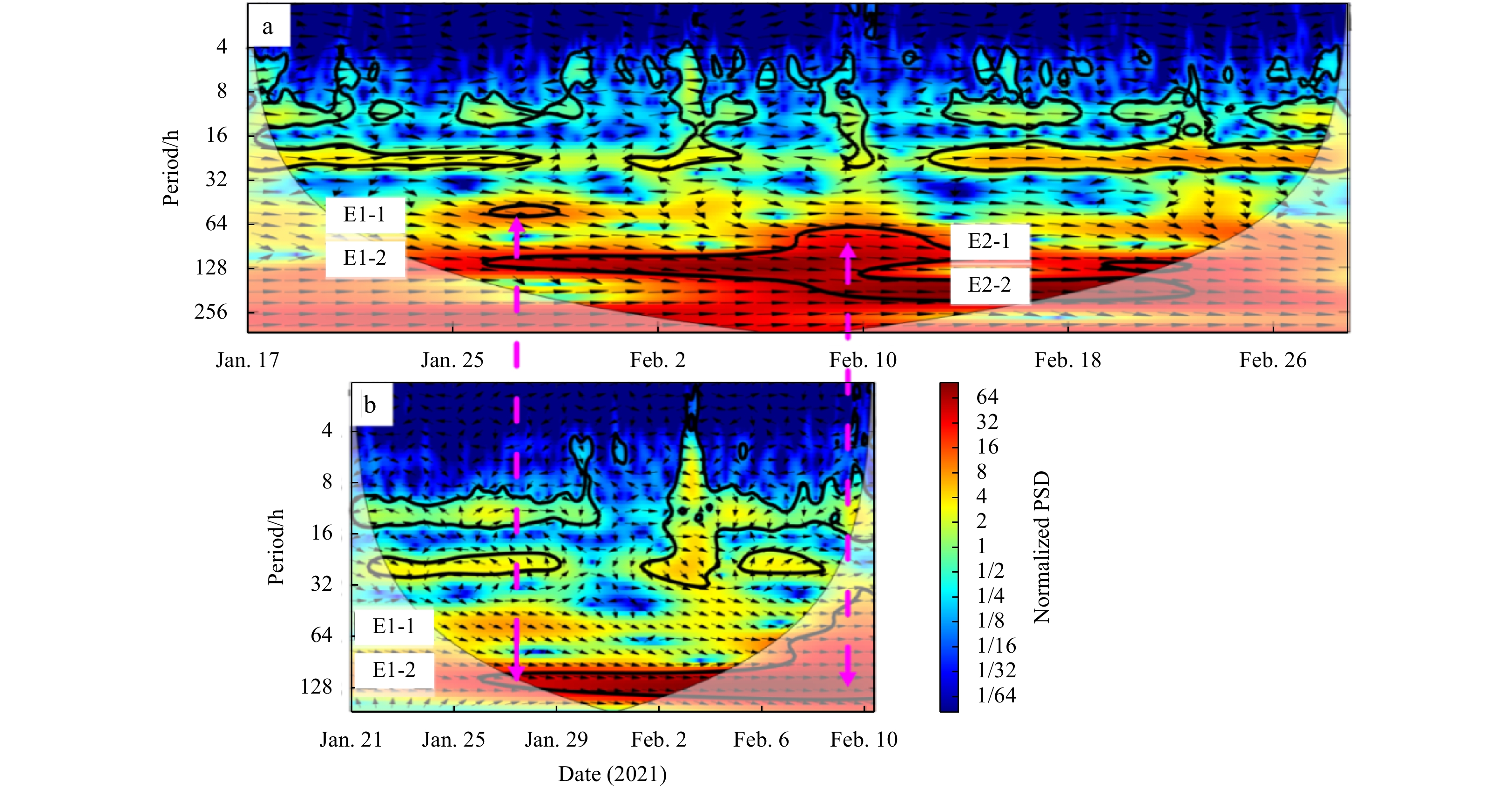
Figures 7a and b show the wavelet transforms of the DSLA at stations ZP and MO. One can see that two prominent sub-inertial events E1 and E2 occurred from January 19 to February 7, and February 8 to 28, respectively. For E1, the power is concentrated at period bands 56 h (E1-1) and 94 h (E1-2). High frequency band E1-1 occurred from January 23 to 30, which maintained for a time interval much shorter than that of E1-2. For E2, the power is peaked at period bands 80 h (E2-1) and 180 h (E2-2). Between February 8 and 10, the power of E2-1 and E2-2 is coincident, indicating that high energy was injected into the ocean. The period of E2-1 increased with time and to 94 h after February 17 (Figs 7a–c).

Figure  7.  Wavelet transforms of DSLA at stations. a. ZP and b. MO, c. along-shelf and d. cross-shelf components of barotropic (BT) current, e. along-shelf and f. cross-shelf components of baroclinic (BC) current at the depth of 14 m. The black and blue dashed lines with arrows and squares point out events and spectral bands. The thick black lines are the 5% significance level against red noise. The power spectrum is normalized, and the unit is 1. The color code represents normalized PSD.

DownLoad: Full-Size Img PowerPoint

The same period bands occur in the wavelet transform of DSLA at HK (not shown here), ZP, MO and barotropic along-shelf current (Figs 7a–c). In the wavelet transforms of barotropic cross-shelf current and baroclinic current (Figs 7d–f), the frequency of high-power spectra peak is inconsistent with that in Figs 7a–c. One can see that the frequencies of E1 and E2 in barotropic cross-shelf current and baroclinic currents are a little lower than that in Figs 7a–c.

Figure 8 shows the bandpass DSLA with periods of 56 h, 94 h and 180 h by a 4-order Butterworth filter. One can see that E1-1 with the amplitude of about 0.07 m occurred from January 17 to February 7. The amplitude of E1-2 is about 0.05 m as shown in Fig. 8b. In this period band, there was a sudden increase close to 0.1 m on February 8, indicating that high energy was injected into the ocean. The amplitude of DSLA in the period band of 180 h also increased from 0.04 m in E1 to 0.9 m in E2.

Figure  8.  Time series of bandpass DSLA at stations HK, ZP, MO and QL with periods of 56 h (a), 94 h (b) and 180 h (c) derived from 4-order Butterworth filter. Dashed lines with shadow point out E1 and E2. Dashed black curves and arrow indicate the propagation of signals in DSLA. A 4-order Butterworth bandpass filter with frequency cutoffs (−3 dB) at 0.34 d⁻¹ and 0.60 d⁻¹ for 56 h period band, 0.20 d⁻¹ and 0.30 d⁻¹ for 94 h period band, 0.11 d⁻¹ and 0.16 d⁻¹ for 180 h period band.

DownLoad: Full-Size Img PowerPoint

Comparing the curves shown in Fig. 8, one can see that the signals in DSLA propagate form HK to QL, i.e., the earliest high peak of DLSA occurred at HK and reached ZP in 5–10 h later. Then, the signals appeared at MO and QL in sequence. Moreover, the signal amplitude is the highest at HK and the lowest at QL, suggesting that the wave energy is dissipated during propagation process.

3.2 Propagation process

Figure 9 shows the XWT of DSLA at station pairs. The periods and phase speeds of the signal derived from XWT are listed in Table 1. The propagation speed of sea level signal is calculated by the lag time of sea level propagation between neighboring stations. One can see that the period band and the occurrence time of the significant cross wavelet power are consistent with that in Figs 6 and 7. Moreover, southwestward propagation of signals from HK to QL shows variable behavior. The phase speed of E1-1 is (13.6 ± 1.6) m/s from HK to ZP and decreases to (8.2 ± 1.1) m/s from ZP to QL. For E1-2, the phase speed is (6.9 ± 4.9) m/s from HK to ZP and increases to (16.7 ± 8.7) m/s from ZP to QL. The phase speed of E1-2 is much slower than that of E1-1 between HK and ZP, while much faster than that of E1-1 between ZP and QL. The wave signal propagates from station HK to ZP at a speed of (18.9 ± 5.1) m/s for E2-1, and (14.5 ± 5.0) m/s for E2-2. For E1-1 and E1-2, the wave signal propagation from ZP to QL is shown in Fig. 9b. One can see that phase speeds are (8.2 ± 1.1) m/s for E1-1, and (16.7 ± 8.7) m/s for E1-2.

Figure  9.  XWT of DSLA for station pairs: HK–ZP (a) and ZP–QL (b). The thick black lines are the 5% significance level against red noise. The thin black lines show the cone of influence (COI). The arrows show the relative phase relationship between two time series with in-phase (anti-phase, leading and lagging) pointing right (left, down and up). Color codes are normalized power spectra. The magenta dashed lines with arrows point out signal events. The power spectrum is normalized, and the unit is 1.

DownLoad: Full-Size Img PowerPoint

Table  1.  XWT of DSLA at different station pairs

Station	Distance/km	Event	Period/h	Time lag/h	Phase speed/(m∙s-1)
HK–ZP	225	E1-1	56	4.6 ± 0.5	13.6 ± 1.6
		E1-2	119	9.1 ± 3.8	6.9 ± 4.9
		E2-1	91	3.3 ± 0.7	18.9 ± 5.1
		E2-2	181	4.3 ± 1.1	14.5 ± 5.0
ZP–QL	174	E1-1	56	5.9 ± 0.7	8.2 ± 1.1
		E1-2	119	2.9 ± 1.0	16.7 ± 8.7

 | Show Table

DownLoad: CSV

The width of continental shelf (from coastline to shelf break of 200 m) between HK−ZP is almost uniform, ~200 km. While, that decreases from 200 km near station ZP to 100 km near station QL. Li et al. (2015) pointed out the width of continental shelf is important to sub-inertial signals over the continental shelf. It seems that the signals propagate faster between HK−ZP than ZP−QL (as shown in Table 1). Shen et al. (2021) pointed out that typhoon-induced sea level signals propagate as fast as (5.6 ± 0.7) m/s near the Taiwan Strait, where the shelf is narrower than that in this study area. Therefore, the wider continental shelf leads a faster signal.

4. Discussion

4.1 Characteristics of CSWs

Hsueh and Romea (1983) found coastal sea level fluctuations with the periods of 48 h, 72 h, and 120 h induced by wintertime wind propagate as barotropic Kelvin waves in the ECS. Chen and Su (1987) pointed out that the SLA signals propagate as CSWs with the phase speed of 16.8 m/s along the coast of the northwestern SCS in winter. The phase speed of sea level signal in this study is ranging from 6.9 m/s to 18.9 m/s, which is comparable with the previous studies. It is noticeable that the signals characterized by this phase speed range show the typical features of CSWs (Ding et al., 2012).

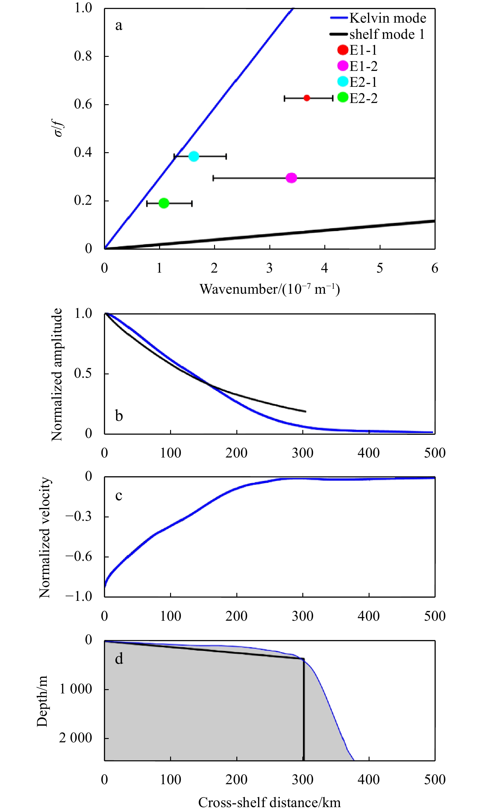
Here we use the toolbox by Brink and Chapman (1985) to calculate the dispersion relation of CSWs with the mean depth profile (as shown in Fig. 10d). The dispersion relation for CSWs in an idealized depth profile (Pedlosky, 1987) is

Figure  10.  Comparison of dispersion relation derived from this study with the Kelvin mode and the lowest mode of CSW (a); arbitrary amplitude of sea level in cross-shelf direction, the amplitude of sea level calculated from the toolbox (blue curve) and that of Kelvin mode (black curve) (b), arbitrary along-shelf velocity component in cross-shelf direction (c), and mean depth profile between ZP and MO (d). The data points in a are calculated from XWT of DSLA for station pairs. For a, theoretical dispersion relations are derived from the mean depth profile (blue curve) as shown in d. Black curve in d represents the idealized depth profile.

DownLoad: Full-Size Img PowerPoint

where $ {J}_{0} $ and $ {J}_{2} $ are the zero and second order of the first kind Bessel function, $ \mu =klf/\omega -F/{\text{γ}} $ and $ F={\left(fl\right)}^{2}/gD $. $ \omega $, $ k $ and ${\text{γ}}$ are wave frequency, wavenumber, ratio of the maximum shelf depth to the deep ocean depth, respectively. f is the Coriolis parameter, $ l $ = 300 km, is the continental shelf width and D is the deep ocean depth. The idealized depth profile for CSWs is the same as the profile by Li et al. (2016), and the parameters are shown in Fig. 10d.

Figure 10a shows comparison of the data derived from XWT of DSLA with the Kelvin mode and mode 1 of CSW. One can see that the data points derived from each station pair are distributed near the dispersion relation of Kelvin mode of the CSW, implying they are the barotropic CSWs. The reason of dispersion relation for E1-2 near the mode 2 may be attributed to the mode mixing and complex mechanism of the generation of CSW (Li, 1993).

The sea level of a Kelvin wave is

where x is distance from coast, c is the phase speed. Figure 10b shows the sea level of Kelvin wave in cross-shelf direction. One can see that the sea level calculated from mean depth profile is in good agreement with the sea level of Kelvin wave. Shen et al. (2021) figured out the cross-shelf structure of CSW using along-track data from satellite altimetry. Both the amplitude of Kelvin wave and CSW show a trapped characteristic of the sea level over the continental shelf. The along-shelf velocity, $ v=\dfrac{g}{f}\dfrac{\partial \zeta }{\partial x} $. As $ \dfrac{\partial \zeta }{\partial x} < 0 $ over the continental shelf, then, $ v < 0 $. Moreover, as the amplitude of the wave shows as an e-exponential curve in Fig. 10b, the along-shelf velocity component would also appear as an e-exponential curve over the continental shelf (shown in Fig. 10c). The maximum along-shelf velocity exists near the coastline, and the current is southward along the coast.

4.2 Signals in along-shelf wind

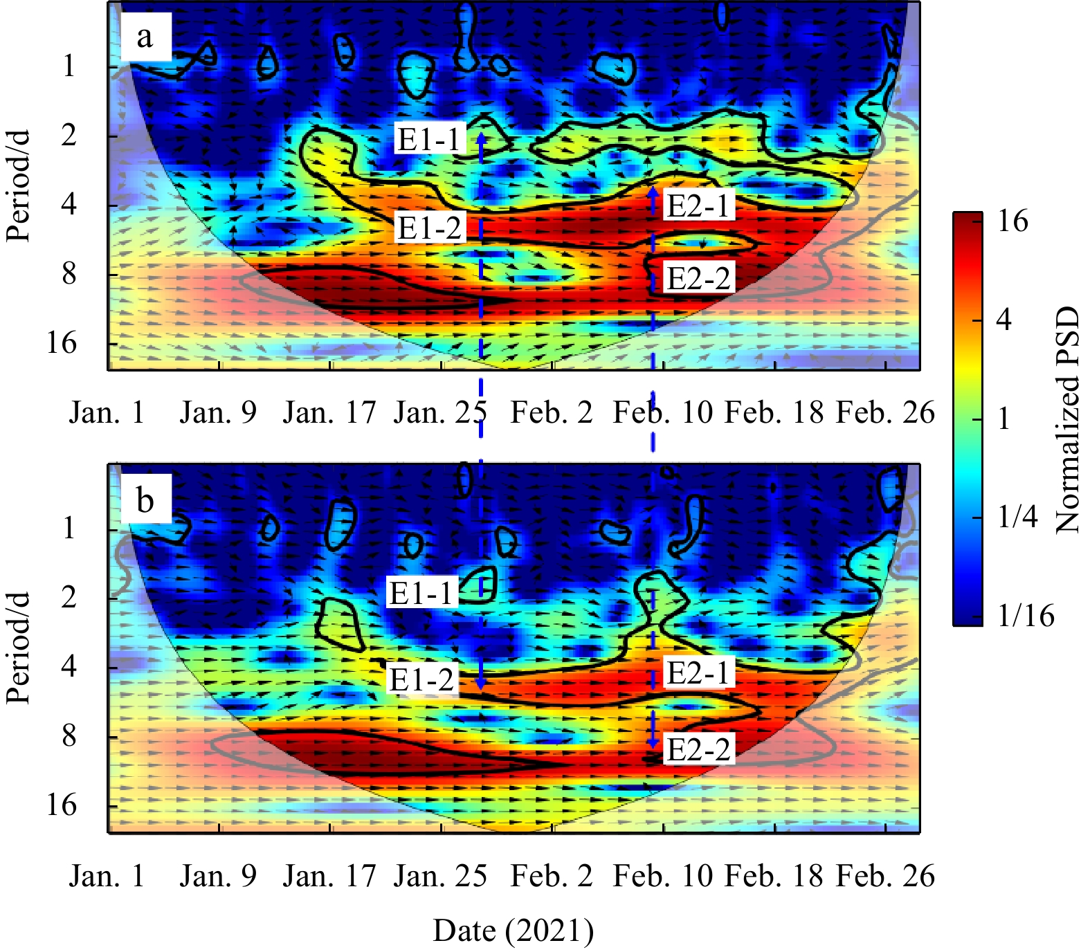
Figure 11 shows XWT of along-shelf sea surface wind at section pairs. The information extracted from XWT is listed in Table 2. One can see that the phase of the along-shelf wind is inconsistent with that of the sea level wave signals. On one hand, the phases of the along-shelf wind propagate along the coast at a mutable speed ranging from –101.4 m/s to 29.0 m/s, much higher than a range of 6.9–18.9 m/s of CSW events E1 and E2. The highest speed of 101.4 m/s implies that the winds between two sections are almost in phase as the time lag is shorter than 1 h. Yang et al. (2016) found that there is no obvious westward propagation signal of wind stress and wind stress curl over the shelf of the NSCS. It indicates that the weather system propagates very fast. That is the reason why such mutably speed was calculated from XWT of alongshore winds. On the other hand, the average wind speed in the study area is about 6 m/s. The maximum is about 15 m/s at W1 and decreases to 10 m/s at W3. The wind speed is a little lower than the phase speed of CSWs.

Figure  11.  XWT of along-shelf velocity component of sea surface wind for section pairs W1–W2 (a) and W2–W3 (b). The thick line is the 5% significance level against red noise. The thin line shows the cone of influence (COI). The arrows show the relative phase relationship between two time series with in-phase (anti-phase, leading and lagging) pointing right (left, down and up). Color codes are normalized power spectra. The blue lines with arrows point out CSW events. The power spectrum is normalized, and the unit is 1.

DownLoad: Full-Size Img PowerPoint

Table  2.  XWT of along-shelf wind at different station pairs

Station	Distance/km	Event	Period/h	Time lag/h	Phase speed/(m∙s−1)
W1–W2	225	E1-1	56	–2.3 ± 0.2	–27.2 ± 2.1
		E1-2	119	3.6 ± 1.2	17.4 ± 4.4
		E2-1	91	–3.9 ± 0.5	–16.0 ± 1.8
		E2-2	181	3.3 ± 0.1	18.9 ± 0.5
W2–W3	73	E1-1	56	–0.2 ± 0.4	–101.4 ± 67.6
		E1-2	119	3.0 ± 0.4	6.8 ± 0.8
		E2-1	91	0.7 ± 0.5	29.0 ± 12.1
		E2-2	181	3.1 ± 0.1	6.5 ± 0.2

 | Show Table

DownLoad: CSV

However, the wind burst in winter is an important generation mechanism for CSW in the coastal China seas (Hsueh et al., 1986). The mean wind speed in E1-2 and E2-2 is comparable to the phase speed of CSWs as shown in Tables 1 and 2. The phase speed of CSW could be forced by the phase speed of wind stress. The dispersion relation of E1-2 deviates theoretical dispersion relations of Kelvin mode obviously as shown in Fig. 10a. Therefore, the wave propagates along the coast with a hybrid form. Thus, the alongshore wind is important to the CSWs.

4.3 Ocean response to the wind

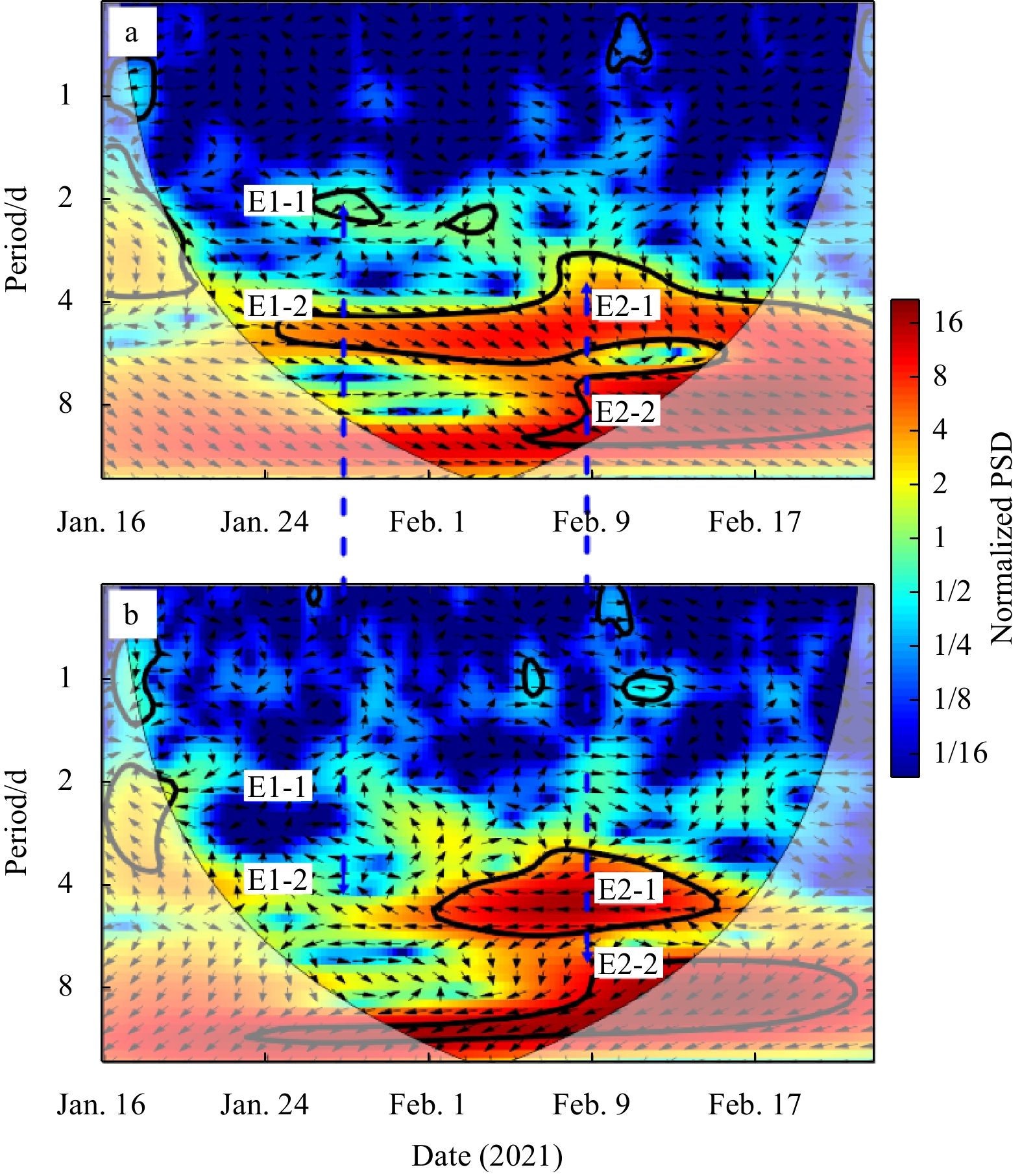
Figure 12 shows XWT of along-shelf wind component with cross-shelf and along-shelf velocity measured at mooring station MO. One can see that two prominent events E1 and E2 occurred in Fig. 12a. The period bands (~50 h, 90 h and 180 h) and occurrence time (from January 20 to February 7, and February 8 to 22) of the significant cross wavelet power are consistent with that in Figs 7–9. The phase lag is about π/4–π/2, which means that the cross-shelf ocean current velocity lags along-shelf wind 10–20 h. It can be speculated that the along-shelf wind drives an onshore Ekman transport in E1 and E2, which generates current convergence and sea level rise near the coast. Figure 12b shows a weak correlation between along-shelf wind and along-shelf current components, especially in E1.

Figure  12.  XWT of along-shelf wind component at section W3 with cross-shelf (a) and along-shelf (b) velocities measured by mooring station MO. The thick line is the 5% significance level against red noise. The thin line shows the cone of influence (COI). The arrows show the relative phase relationship between two time series with in-phase (anti-phase, leading and lagging) pointing right (left, down and up). Color codes are normalized power spectra. The blue dashed lines with arrows point out CSW events. The power spectrum is normalized, and the unit is 1. The color code represents normalized PSD.

DownLoad: Full-Size Img PowerPoint

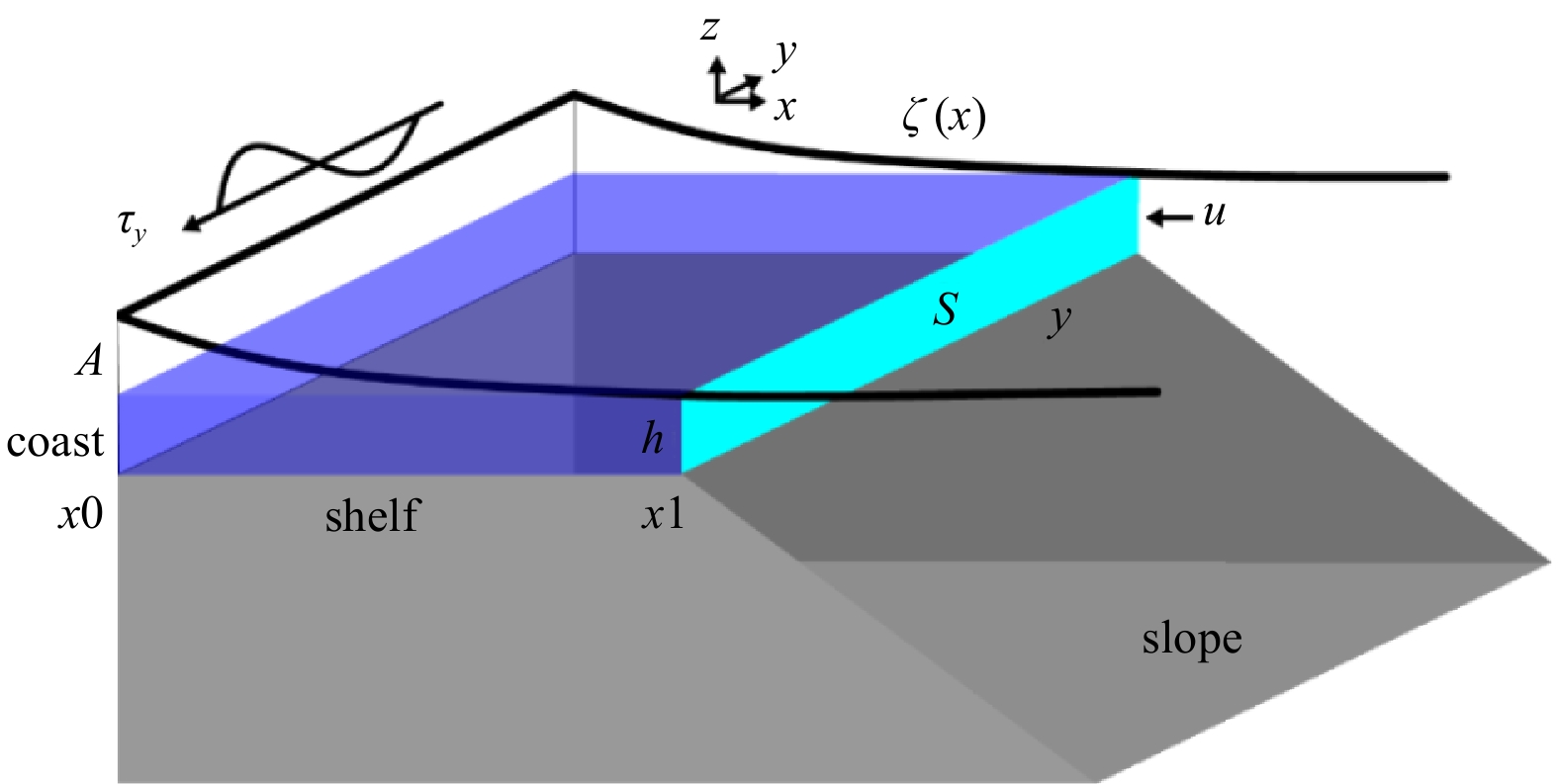
To further examine the ocean response to the wind forcing, we assume the sea surface fluctuation is balanced with the flux of Ekman transport induced by the along-shelf sea surface wind stress as shown in Fig. 13.

Figure  13.  Sketch of the wind-driven sea surface fluctuation and Ekman transport over the continental shelf.

DownLoad: Full-Size Img PowerPoint

where $ \zeta $ is sea surface fluctuation in the cross-shelf direction. u ($ =-{\tau }_{y}/\rho_{\mathrm{w}} fh) $ is the Ekman current velocity. $ {\tau }_{y} $ is along-shelf wind stress, h is water depth at the continental shelf edge, S (= hy) is the flux section at the continental shelf edge, x0 and x1 are the ranges of wind action on the sea surface in cross-shelf direction, t0 and t1 are the duration of wind action on the sea surface.

Suppose that horizontal distribution of the sea surface fluctuation induced by the along-shelf wind stress is in the form of an exponential function, i.e., $\zeta\left(x\right)=A\;\mathrm{e}\mathrm{x}\mathrm{p}\left(-fx/c\right)$, here c is the phase speed of CSW, and the along-shelf wind stress is independent of x over the continental shelf, i.e., $ {\tau }_{y}=-{\tau }_{0}\;\mathrm{sin}\left(k_{\mathrm{a}}y+\omega t\right) $, where $ {\tau }_{0} $ is the maximum wind stress, k_a is wavenumber in the along-shelf direction, and $ \omega $ is the wind stress frequency. $ {\tau }_{y} $ is negative in winter over the shelf of the NSCS, i.e., $ {\tau }_{y} < 0 $. Substituting $ \zeta \left(x\right) $ and $ {\tau }_{y} $ into Eq. (12), the sea surface fluctuation A is calculated as

where $ \phi =k_{\mathrm{a}} \cdot y+\omega \cdot t1 $, x1 is the width of continental shelf. Variable t1 is a time interval between breezeless ($ {\tau }_{y}=0 $) and the arbitrary ($ {\tau }_{y} $) of wind stress. In Eq. (13), the sea level fluctuation is expressed as the phase angle of wind stress, $ \phi $, which means that we could use the relationship of phase angle between wind stress and sea level to calculate the sea level. This method is convenient as the phase angle could be directly extracted from XWT of along-shelf wind stress and sea level (or the current component).

We apply the Eq. (13) to calculate the low-frequency sea level fluctuation at the coast area using the wind stress. In the study area, let y = 1, h = 330 m, x0 = 0 km, x1 = 300 km (Fig. 11d). t0 = 0 s, and t1 is the time lag between cross-shelf current and along-shelf wind stress, i.e., phase lag in Fig. 12a.

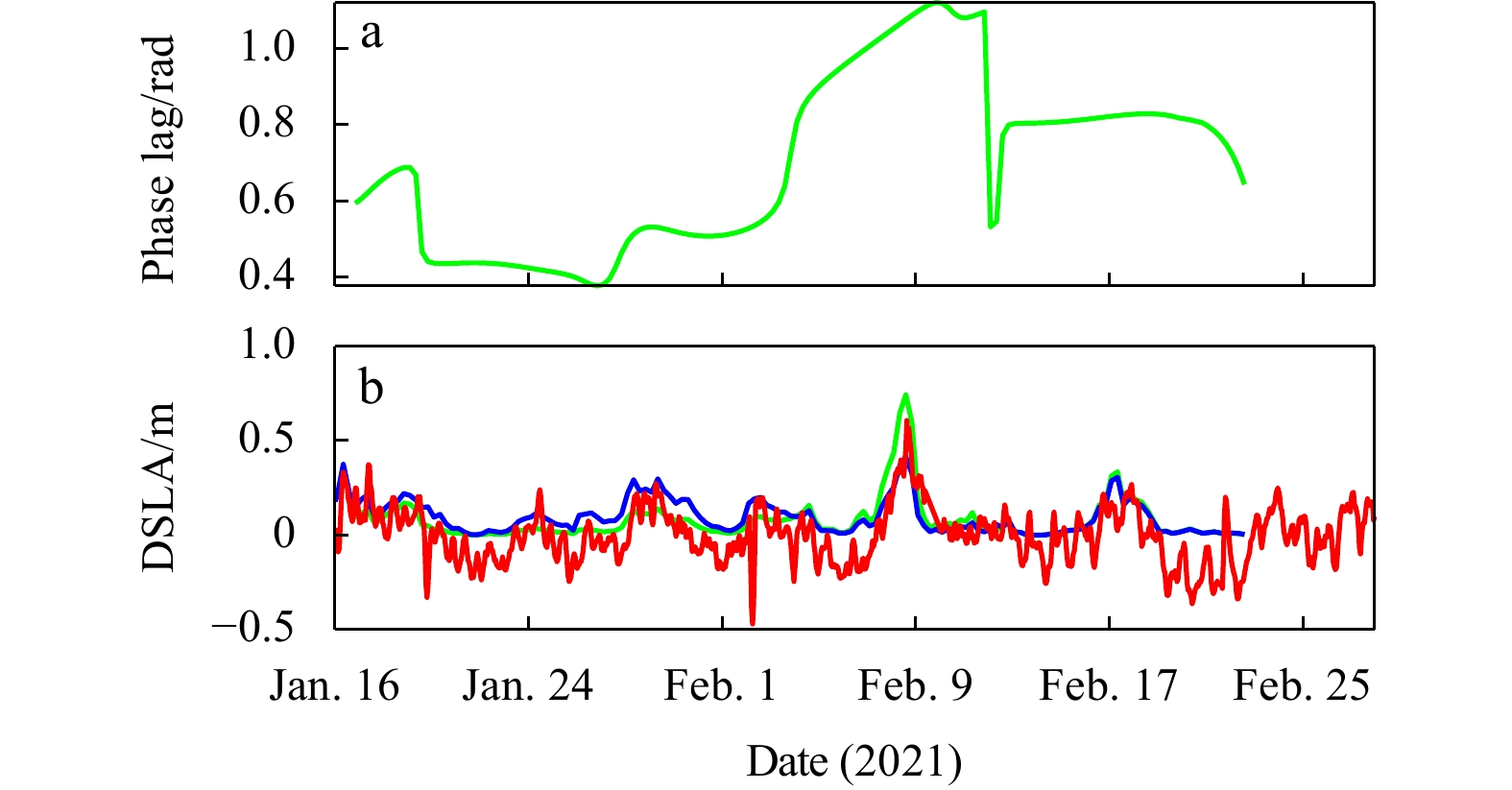
Figure 14 shows the comparison of the DSLA at station ZP and amplitude of sea surface fluctuation calculated using time series of along-shelf wind. When the major northerly wind pulses appear on February 8, the sea level calculated with the phase lag from Fig. 14a reached the peak of 0.7 m, and the DSLA at station ZP was 0.6 m, resulting in an overestimation of about 17%. It would underestimate the sea level if using a fixed phase of π/4. The results shown in Fig. 14 indicate that sea surface fluctuation agrees well with that calculated by the Kelvin mode. Therefore, the sea level fluctuations are mainly controlled by the Kelvin mode in this study.

Figure  14.  Phase lag between sea surface fluctuation and along-shelf wind from Fig. 12a (a); comparison of the DSLA at station ZP (red curve) with amplitude of sea surface fluctuation with the fixed phase of π/4 (blue curve), and amplitude of sea surface fluctuation (green curve) calculated with the phase lag in a (b).

DownLoad: Full-Size Img PowerPoint

4.4 Ocean baroclinic response

Based on a long-wave assumption of CSW, the scale of the along-shelf length of CSW ($ L=2\pi /k_{\mathrm{a}}\approx 2\times {10}^{3}\;\mathrm{k}\mathrm{m} $) is much larger than cross-shelf length ($ l=200\;\mathrm{k}\mathrm{m} $), i.e., $ l/L\ll 1 $. Thus, for the linearized shallow-water equations, we approximately take that $ \partial u/\partial t=0 $ (Li et al., 2016). The linearized, hydrodynamics with the long-wave assumption could be solved over an idealized bathymetry model (Schulz et al., 2012). However, PSD of de-tided cross-shelf baroclinic current is much larger than that of along-shelf component as shown in Figs 6b and c, implying that cross-shelf velocity is an essential component for the theoretical analysis of CSW.

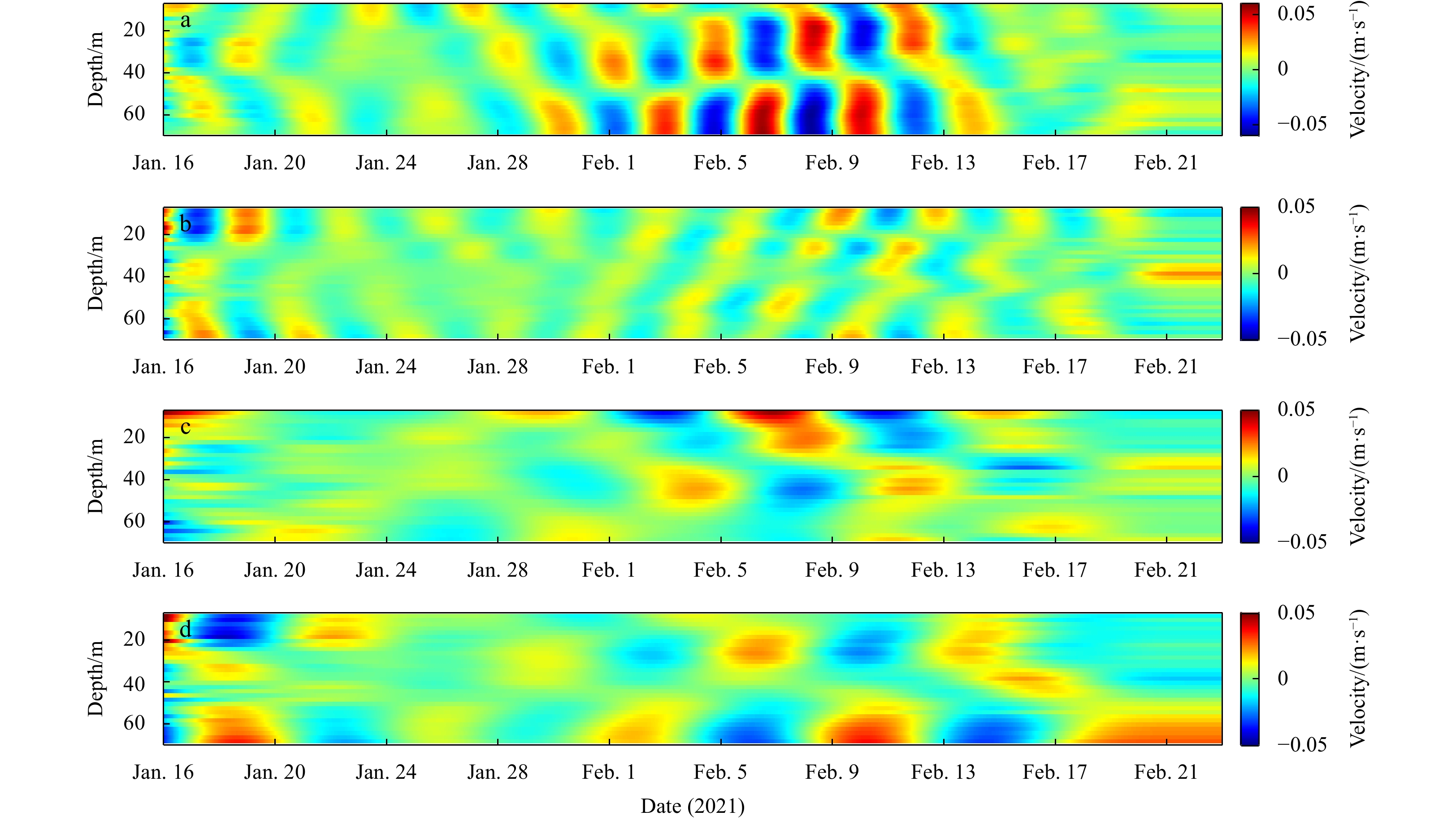
Figure 15 shows bandpass of cross-shelf and along-shelf velocity components with period of 90 h and 190 h derived from 4-order Butterworth filter. In E1, the along-shelf velocity signals with the period of 90 h and 190 h were as high as 0.05 m/s, which was much higher than that in cross-shelf velocity component. In E2, however, especially in February 9, the cross-shelf velocity component with the period of 90 h was as high as 0.07 m/s and the along-shelf velocity component was only about 0.03 m/s. The magnitudes of cross-shelf and along-shelf velocity are comparable with that for the period band of 190 h in E2. The high cross-shelf velocity in E2 would result from the variability of the alongshore wind as shown in Fig. 5b. The effect of violently changing in cross-shelf wind should be clarified in further study.

Figure  15.  Bandpass cross-shelf current (a), along-shelf current velocity (b) distribution with a central period of 90 h, and bandpass cross-shelf current (c) and along-shelf current velocity (d) distribution with a central period of 190 h.

DownLoad: Full-Size Img PowerPoint

In addition, the mode 2 CSW could be seen clearly from the cross-shelf velocity components in E1 and E2 as shown in Fig. 15. Previous studies presented that the progress of CSW is barotropic in the study area in winter (Ding et al., 2012; Li et al., 2016). However, the bandpass currents indicate that the baroclinic CSW is as important as the barotropic progress in the northwest SCS, although the baroclinic CSW is not embodied in the DSLA. From Fig. 4, one can see that there is a strong thermohaline front in the area with the depth of 60 m. The extremal peak of buoyancy frequency occurred in the depth of 20 m, and extended to the depth of 40 m near the front. The cold and light water caused strong baroclinic CSWs is distributed on the coastal side of the study area.

5. Summary and conclusions

In this study, cruise and mooring observations and tidal gauge data at stations HK, ZP and QL from January 1 to February 28, 2021 are used to investigate the characteristics of sub-inertial CSWs in the northwestern continental shelf of the SCS. The sea surface wind data are used to examine the relationship between along-shelf wind and sea level fluctuation. Driven by the along-shelf winds, two CSW events are detected from wavelet spectra of DSLA in the sub-inertial period band. The CSW signals are triply peaked at periods of 56 h, 94 h and 180 h (0.0177 h⁻¹, 0.0106 h⁻¹ and 0.0056 h⁻¹), propagating along the coast with phase speed ranging from 6.9 m/s to 18.9 m/s. The dispersion relation indicates that the signal property belongs to the Kelvin mode of CSW.

The cruise data analysis results show that the along-shelf wind drives an onshore Ekman transport, which drives ocean current convergence onto the coast. Meanwhile, the results show a weak correlation between along-shelf wind and along-shelf current. Thus, the amplitude of sea surface fluctuation may be estimated by the along-shelf wind. The results are comparable with the observation data. In addition, the mode 2 CSW could be seen from the cross-shelf current component measured from a single mooring station. Of course, a cross-shelf mooring array should be the best way to overcome limitations of single mooring for observing the cross-shelf structures of CSWs.