Jianbo Cui, Yunhua Wang, Yanmin Zhang, Huimin Li, Wenzheng Jiang, Yushi Zhang, Xin Li. A new model for Doppler shift of C-band echoes backscattered from sea surface[J]. Acta Oceanologica Sinica, 2023, 42(6): 100-111. doi: 10.1007/s13131-022-2144-8
Citation:
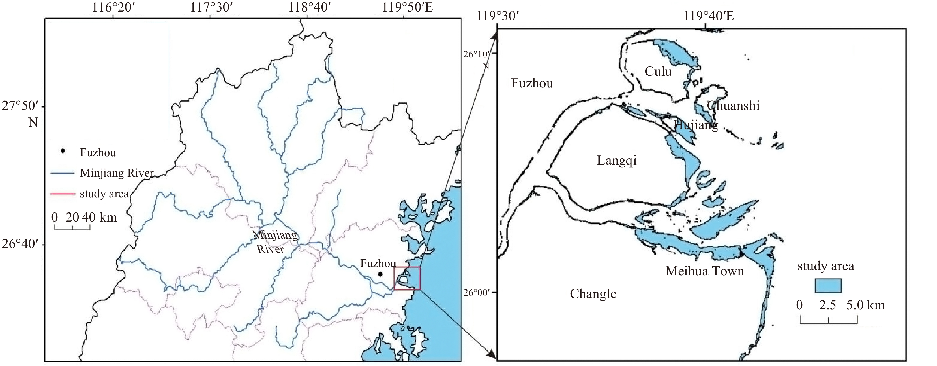
Xiaohe Lai, Chuqing Zeng, Yan Su, Shaoxiang Huang, Jianping Jia, Cheng Chen, Jun Jiang. Vulnerability assessment of coastal wetlands in Minjiang River Estuary based on cloud model under sea level rise[J]. Acta Oceanologica Sinica, 2023, 42(7): 160-174. doi: 10.1007/s13131-023-2169-7
Jianbo Cui, Yunhua Wang, Yanmin Zhang, Huimin Li, Wenzheng Jiang, Yushi Zhang, Xin Li. A new model for Doppler shift of C-band echoes backscattered from sea surface[J]. Acta Oceanologica Sinica, 2023, 42(6): 100-111. doi: 10.1007/s13131-022-2144-8
Citation:
Xiaohe Lai, Chuqing Zeng, Yan Su, Shaoxiang Huang, Jianping Jia, Cheng Chen, Jun Jiang. Vulnerability assessment of coastal wetlands in Minjiang River Estuary based on cloud model under sea level rise[J]. Acta Oceanologica Sinica, 2023, 42(7): 160-174. doi: 10.1007/s13131-023-2169-7
Department of Water Resources and Harbor Engineering, College of Civil Engineering, Fuzhou University, Fuzhou 350108, China
2.
Fujian Institute of Geological Survey, Fuzhou 350108, China
Funds:
The National Natural Science Foundation of China under contract No. U22A20585; the Education Research Project of Fujian Education Department under contract No. JAT200019.
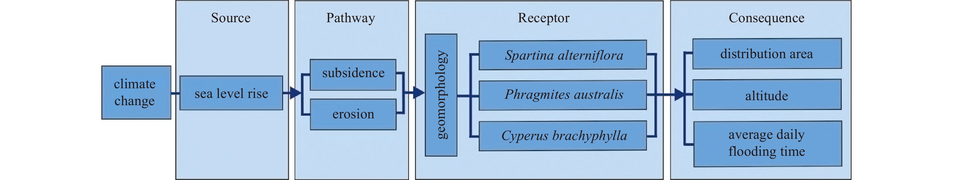
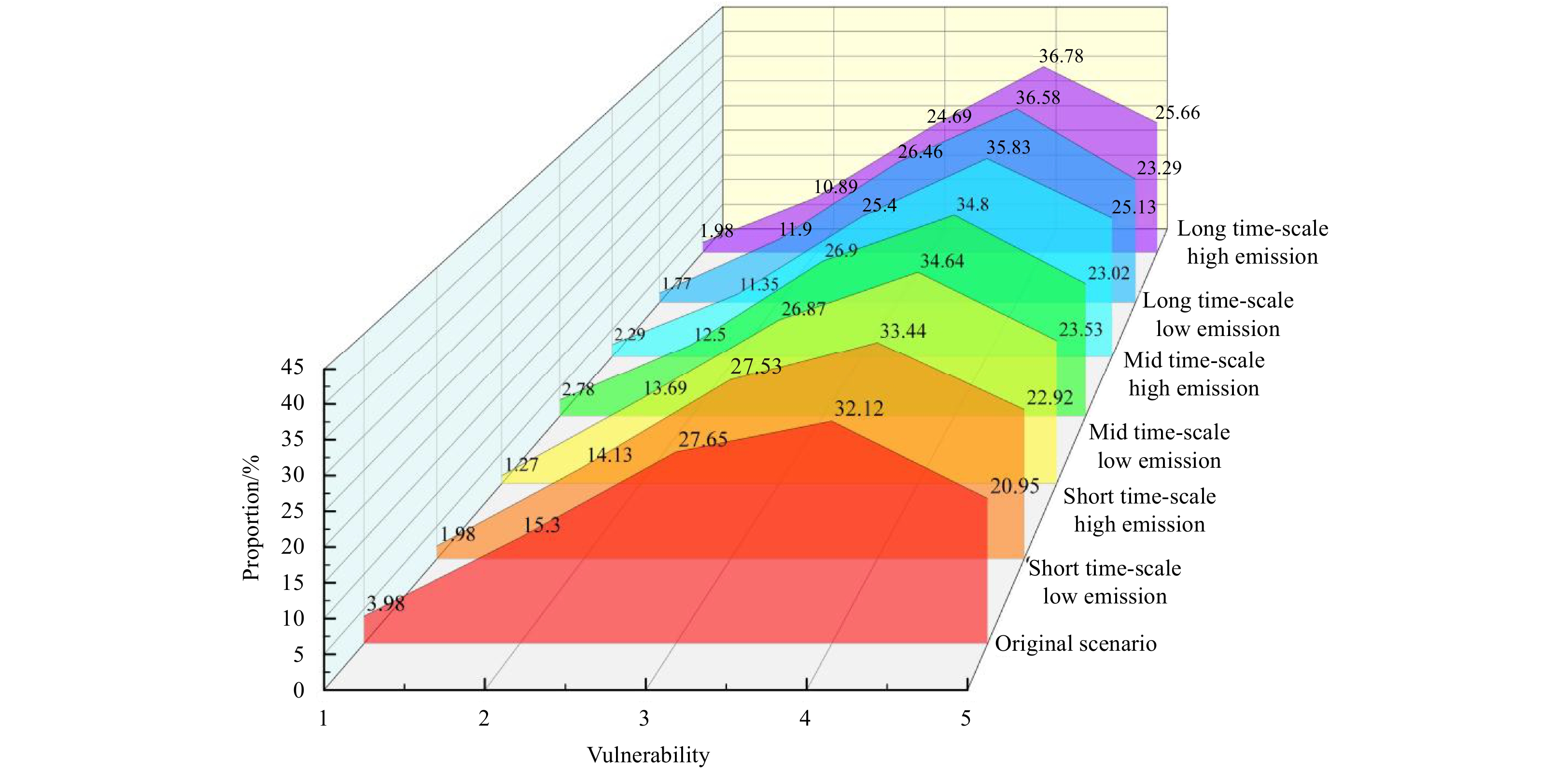
The change of coastal wetland vulnerability affects the ecological environment and the economic development of the estuary area. In the past, most of the assessment studies on the vulnerability of coastal ecosystems stayed in static qualitative research, lacking predictability, and the qualitative and quantitative relationship was not objective enough. In this study, the “Source-Pathway-Receptor-Consequence” model and the Intergovernmental Panel on Climate Change vulnerability definition were used to analyze the main impact of sea level rise caused by climate change on coastal wetland ecosystem in Minjiang River Estuary. The results show that: (1) With the increase of time and carbon emission, the area of high vulnerability and the higher vulnerability increased continuously, and the area of low vulnerability and the lower vulnerability decreased. (2) The eastern and northeastern part of the Culu Island in the Minjiang River Estuary of Fujian Province and the eastern coastal wetland of Meihua Town in Changle District are areas with high vulnerability risk. The area of high vulnerability area of coastal wetland under high emission scenario is wider than that under low emission scenario. (3) Under different sea level rise scenarios, elevation has the greatest impact on the vulnerability of coastal wetlands, and slope has less impact. The impact of sea level rise caused by climate change on the coastal wetland ecosystem in the Minjiang River Estuary is mainly manifested in the sea level rise, which changes the habitat elevation and daily flooding time of coastal wetlands, and then affects the survival and distribution of coastal wetland ecosystems.
As the scattering elements on sea surface are moving under the actions of wind, waves and current, the frequency of a radar signal backscattered from oceanic surface thus experiences a Doppler shift, which is proportional to the line-of-sight velocity of the scattering facets and weighted by their backscattered power (Keller et al., 1986). Consequently, the Doppler features could provide information on the ocean dynamic conditions, in complement to the normalized radar cross section (NRCS) which is related to the surface roughness. Thus, the studies on Doppler features are of practical importance in a number of research areas such as sea surface wind retrieving, sea waves monitoring and oceanic surface current measuring (Chapron et al., 2005; Johannessen et al., 2005; Kudryavtsev et al., 2005; Karaev et al., 2008; Johnson et al., 2009). In recent years, the properties of Doppler spectrum from sea surface have been the subject of extensive investigations, both theoretically and experimentally (Crombie, 1955; Bass et al., 1968; Wright and Keller, 1971; Barrick, 1977; Lipa, 1978; Mouche et al., 2008).
On the theoretical side, Crombie (1955) first investigated the properties of Doppler spectrum based on Bragg theory in the early stage. In Barrick (1977), Barrick built a perturbative model based on a representation of sea waves up to second order, which has been widely used for HF and VHF radars. For microwaves, besides the Bragg theory, the Kirchhoff approximation (KA) and the small slope approximation (SSA) can also be used to predict the Doppler shift of the signals from sea surface (Mouche et al., 2008). However, it should be pointed out that the Doppler shift predicted by the Kirchhoff approximation method (KA), the Bragg theory, and the first-order small slope approximation (SSA-1) in co-polarized configuration are insensitive to the polarization state. And experiment results show that the Doppler shift of horizontally polarized signals are generally larger than those vertically polarized case. Bass et al. (1968) and Wright and Keller (1971) established a two-scale surface scattering model (TSM) which includes modulation by the large scale waves, and makes the results closer to the real sea surface situation. What’s more, the polarization dependence of the Doppler shift can also be well explained by using the two scale surface scattering model. In Wang and Zhang (2011) and Wang et al. (2012, 2013), the differences between co-polarized have been explained by the TSM, and the effects of tilt and hydrodynamic modulation have also been analyzed, which gives a quantitative interpretation of Doppler shift of sea surface echo. Up to now, the two-scale surface model is still as the most practical model to theoretically describe the Doppler spectrum of microwave scattering from sea surface (Zavorotny and Voronovich, 1998; Fuks and Voronovich, 2002). In several researches (Zavorotny and Voronovich, 1998; Fuks and Voronovich, 2002; Wang and Zhang, 2011 ; Wang et al., 2012, 2013), however, it should be pointed out that the local NRCS is calculated by the Bragg scattering theory. As we all know, the scattering coefficient calculated by the Bragg scattering theory generally has an obvious discrepancy with the actual signal backscattered from sea surface in real condition. Compared with the Bragg scattering theory, for a specific radar frequency band, the empirical geophysical model function (GMF) can be used to estimate the NRCS backscattered from sea surface more accurately (Verspeek et al., 2012; Li and Lehner, 2014; Mouche and Chapron, 2015; Shao et al., 2016).
In recent years, the numerical methods were also employed to investigate the Doppler spectra of backscattering from one-dimensional sea surfaces (Toporkov and Brown, 2000; Johnson et al., 2001; Hayslip et al., 2003). At low grazing angles (LGA), Toporkov et al. found that the results of numerical simulations showed an obvious broadening of the bandwidth for nonlinear surfaces and a separation of the vertical and horizontal polarization spectra (Toporkov and Brown, 2000). But for the linear sea surface, this spectral separation cannot be observed. Further, the influences of the hydrodynamic models on the Doppler spectra of L-band backscattered fields have been discussed by Johnson and Hayslip et al. (Johnson et al., 2001; Hayslip et al., 2003). In spite of the advantages of the numerical methods, several questions should be mentioned as following: on the one hand, in order to obtain exact numerical results, Doppler simulations turn out to be quite computationally expensive; on the other hand, the influences of different factors, such as hydrodynamic modulation, tilt modulation of large scale waves and so on cannot be assessed individually.
In addition to the theoretical and the numerical methods, a serious of the empirical Geophysical Model Functions (GMF) based on the Doppler shift observations combined with wind and sea state information have been developed in recent studies. For instance, a C-band empirical geophysical model function (CDOP) has been built for estimating wave-induced Doppler shift (Mouche et al., 2012). On the basis of the observed Doppler shift by Sentine-l SAR, another empirical geophysical model, called CDOP-3S which combined wave information into the model, was established by Moiseev et al. (2020). However, the CDOP-3S model performs an overfit of the empirical GMF during training. A new GMF called CDOP-3SiX has been trained based on the coastal data set in Moiseev et al. (2022). Due to addition of the sea wind and swell information, the CDOP-3SiX improves the accuracy of sea state contribution estimates compared to CDOP model. Although the development of the empirical geophysical model function can significantly facilitate the application of the Doppler information in ocean remote sensing. However, the accurate of the empirical geophysical model depends on the sensor’s performance and optimal instrumental configurations. In addition, the empirical models are not easily used to analyze the physical mechanisms that affect the Doppler properties.
To progress in such investigations, our purpose in this paper is to numerically evaluate the wind induced Doppler shift of the echoes backscattered from sea surface by combining the TSM model and nonlinear sea wave model. Predictions will help to better understand the influence mechanism of incidence angle, polarization sensitivities, and modulation effects of large scale waves. What’s more, in this study, the scattering coefficient in the TSM is calculated by the empirical CSAR model (Mouche and Chapron, 2015) rather than Bragg model to get more accurate results. Numerical results show that the Doppler shift of the C-band sea echoes at moderate incidence angles can be well predicted by the method in this work. In order to facilitate the application, a semi-empirical CSAR-DOP model is also developed based on the predicted Doppler shift in this work. In the following section, the numerical theory for Doppler shift is presented in Section II. The results of the numerical models are analyzed in Section III. Using the predicted Doppler shift, a polynomial fitting formula (CSAR-DOP model) is developed in Section IV. The concluding remarks and perspectives are provided in Section V.
2.
The Doppler shift predicted by TSM
2.1
The two-scale scattering model
As the most practical model for theoretical description of microwave Doppler spectrum from sea surface, the two- scale model can be used to give a qualitative and quantitative interpretation of the Doppler shift. In TSM model, sea surface is artificially partitioned into small- and large-scale waves, such that
where $ x,y $ and $ t $ are spatial (horizontal and vertical) and time coordinates, respectively. $ {Z_l}(x,y,t) $ represents the large-scale portion of the surface elevation. $ {Z_s}(x,y,t) $, which has been modulated by large-scale waves, denotes small-scale roughness with $2{k_{\text{e}}}{{\cos}}\; {\theta _i}{Z_s}(x,y,t) \ll 1.0$. $ {k_{\text{e}}} $ is the wave number of microwave and ${\theta _i}$ denotes the incidence angle. If we assume that $ {Z_l}(x,y,t) $ and $ {Z_s}(x,y,t) $ are statistically independent, the total wave-height spectrum, i.e., $ W( {{\boldsymbol{K}}} ) $, can be written as
where $ {W_{ms}}( {\boldsymbol{K}} ) $ and $ {W_l}( {\boldsymbol{K}} ) $ denote the wave-height spectra corresponding to small- and large-scale surface roughness. In this work, the two-dimensional spectrum proposed by Elfouhaily et al. (1997) is selected for the large-scale sea waves.
According to the linear theory, the sea surface can be described as a sum of large number of harmonics with different amplitudes, frequencies, and random phases. However, if we aim at studying radar Doppler character, the nonlinearities of actual sea surface cannot be neglected, especially, the skewness properties would induce obvious effect on the Doppler shift. In general, the nonlinear sea surface can be expanded in perturbation series. The first order perturbation term corresponds to the linear surface and the higher order corrections come from the expansion of the hydrodynamic formulas in terms of wave interactions. For large-scale waves, the narrow-band assumption is acceptable. On the basis of this narrow band assumption, Tayfun (1986) proposed a nonlinear sea surface model, which results in a random sea surface whose crests are narrow and peaked, and whose troughs are long and flat. Such asymmetry of the vertical direction is referred to as vertical-skewness. At the same time, the horizontal-skewness, which directly affects the surface slope distribution, also occurs in sea waves. In Fung (1994), Fung found that, compared to vertical-skewness, the horizontal-skewness induces more remarkable influence on backscattered signal. The Lagrange Model with linked components (hereinafter referred to as LMLC) is an optional hydrodynamic model for the nonlinear water waves (Lindgren, 2009; Lindgren and Åberg, 2009). The LMLC model can produce the realistic vertical- and horizontal-skewness. For two-dimensional deep water waves, the LMLC can be written as
where $ {x_{\text{0}}} $ and $ {y_{\text{0}}} $ are the abscissa and ordinate of the water particle’s equilibrium position. And $ F\left( {{K_{xm}},{K_{yn}}} \right) $ denotes the Fourier coefficients of sea surface profile, the wavenumber and the angular frequency are $ {K_{mn}} = \sqrt {K_{xm}^2 + K_{yn}^2} \leqslant {K_{{\text{cut}}}} $ and $ {\omega _{mn}} = \sqrt {g{K_{mn}}} $ with ${K_{xm}} = {{2\pi \left( {m - {M /2}} \right)} / {{L_x}}}$, ${K_{yn}} = 2\pi {{\left( {n - {N / 2}} \right)} / {{L_y}}}$. $ {K_{{\text{cut}}}} $ denotes the cut-off wavenumber. ${L_x}$ and ${L_y}$ are the lengths of sea surface along $ \hat x $ and $\hat y$ directions, $m = 1,2, \cdots, M$; $n = 1,2, \cdots, N$. The linking parameter ${\alpha _{mn}} = {\text{γ}} /\omega _{mn}^2$, and ${\text{γ}} $ can be defined by the relation between the horizontal acceleration of the water particles and the vertical displacement (Lindgren, 2009; Lindgren and Åberg, 2009).For narrow-band waves, ${\text{γ}} = 0$ and $ {\text{γ}} = \omega _{mn}^2 $ correspond to the nonlinear sea surface models proposed in Tayfun (1986) and Chen et al.(1993), respectively. In Lindgren and Åberg (2009) and Lindgren (2009), Lindgren set ${\text{γ}} = 0.4$ or 0.8 for horizontal-skewness water waves. However, strong correlation between the biphase $ {\ \beta _{mn}} = {{\arctan}} \left( {{\text{γ}} /\omega _{mn}^2} \right) $ and wind forcing was found by Leykin et al. (1995) through the experiment in a laboratory wave tank under varied wind conditions. But, so far, few data measured from actual situation can be directly compared with the results obtained by Leykin and Donelan et al. (Leykin et al., 1995). In this work, we set ${\text{γ}} = 0.4$. Because the difference of the orbital velocity for linear and nonlinear large scale waves only has negligible influence on the Doppler properties, for simplicity, the orbital velocity components in different directions are still simulated based on the linear wave model, i.e.,
The small-scale roughness of sea waves would be modulated by the large-scale underlying waves, and the spatial variation of $ {W_{ms}}( {\boldsymbol{K}} ) $ induced by the hydrodynamic modulation of large-scale waves can be written as
where $ {W_s}( {\boldsymbol{K}} ) $ denotes the roughness spectrum which is not modulated by large-scale waves. And the hydrodynamic modulation transfer function ${M_{{\rm{hydr}}}}$ takes the form as Alpers et al. (1981),
where $ {{\boldsymbol{K}} _l} $ and $ {{\boldsymbol{K}} _s} $ denote the wavenumbers of large- and small-scale waves, respectively. $\mu $ is the relaxation rate and has to be determined by experiment. For $ \mu=0 $, the maximum of the short wave energy occurs at the crests of the large-scale waves. However, the fact is that a nonvanishing phase shift between the maximum of the short wave spectral energy and the large-scale waves’ crest exists, which yields a different scattering coefficient when radar looks along the upwind and downwind directions. As discussed in Wang et al. (2016), the hydrodynamic modulation of large-scale waves is more significant with wind speed. Thus a reasonable Doppler shift could be obtained by relating the wind speed to the relaxation rate $ \mu $, characterized by setting the nonvanishing phase shift to be about $ \pi /4 $ (i.e., $ \mu {\text{ = }}{\omega _{\text{p}}} $), representing the angle frequency of the spectral peak wave. Thus, based on the two-scale model, the scattering coefficient from each facet on the large scale waves can be expressed as
In the traditional two-scale model, the scattering coefficient $\overline {{\sigma _{{\rm{PP}}}}({\theta '_i})}$ in Eq. (11) is evaluated by the Bragg theory. However, as an analytical approximation method, the Bragg resonance scattering method cannot accurately describe the backscattering field from sea surface. Therefore, in the present work, the dual-polarized C-band empirical geophysical model function (CSAR model) (Mouche and Chapron, 2015) is employed to evaluate the scattering coefficient $\overline {{\sigma _{{\rm{PP}}}}({\theta '_i})}$. The subscript PP represents HH or VV polarization. The local incidence angle $ {\theta '_i} \approx {\theta _i} - {S_l} $, $ {\theta _i} $ is the incidence angle, the slope of the large scale waves along radar look direction is
where ${\varphi _i}$ denotes the azimuth angle of the radar beam (i.e., the angle between radar beam direction and x-axis direction).
2.2
The Doppler centroid frequency shift
Doppler centroid frequency shift ${ (f_D) }$ can be generally considered as the first-order moment of Doppler spectrum and weighted by scattering power. First of all, at moderate incidence angles, the microwave scattering field from sea surface is dominated by resonant Bragg scattering, thus the phase speed of the short Bragg resonant water waves would yield a partial Doppler shift. Accordingly, the corresponding Doppler spectrum would consist of two spectral peaks resulting from the phase speed of the Bragg wave components traveling toward and away from radar. However, under actual sea conditions, these spectral peaks are not only broadened but also shifted due to the modulation effect of the large-scale waves. Considering the effect of the tilt and the hydrodynamic modulation of the large-scale waves, the additional Doppler centroid frequency shift ${(f_M)}$ can be evaluated by
where the velocities $ {V_x}_{mn} $, $ {V_{ymn}} $ and $ {V_z}_{mn} $ can be evaluated by Eqs (6)−(8). Based on the Bragg scattering and the modulation of Bragg waves by longer waves, the Doppler centroid frequency shift of the microwave echoes backscattering from sea surface can be written as
where the wind drift ${{\boldsymbol{U}} _{{\text{drift}}}}{\text{ = }}0.03{{\boldsymbol{U}} _{10}}$ and $ {{\boldsymbol{U}} _{10}} $ denotes the wind speed at a height of 10 m above sea surface. ${{\boldsymbol{K}} _{\text{B}}}$ is the wave number of Bragg wave, $ {\phi _{\text{B}}} $ denotes the azimuth angle of the Bragg wave. $ F(K,\phi ) $ denotes the angle spread function (Apel, 1994).
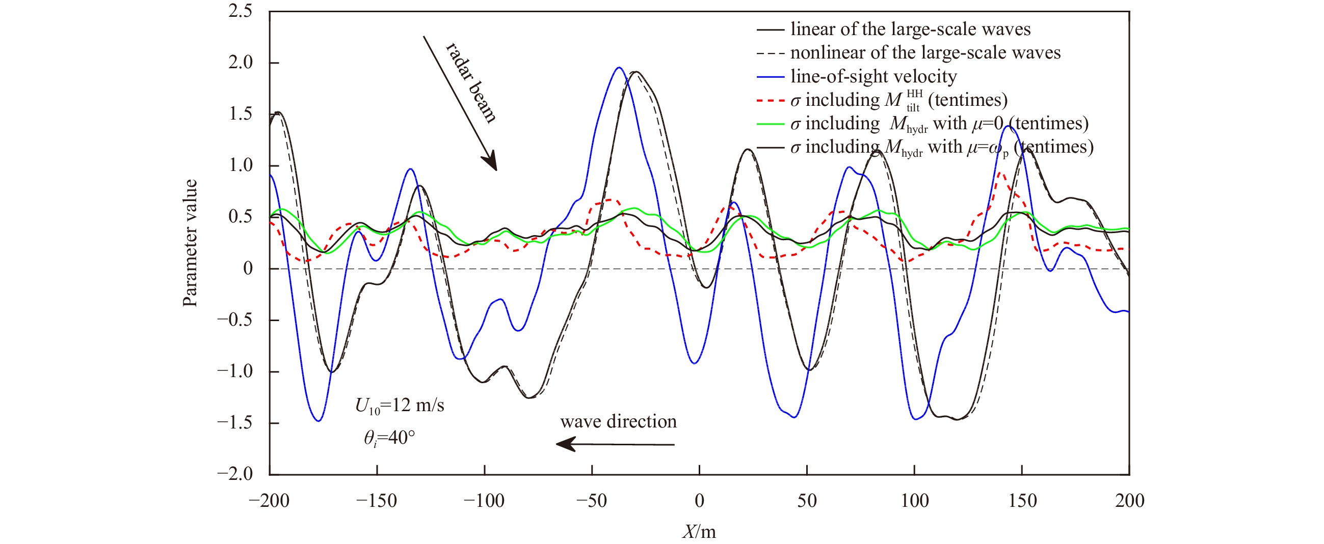
From Eqs (13) and (14) we can find that the predicted Doppler centroid frequency shift would be affected by the locally-modulated radar cross section and the orbital motions of the large-scale waves. Figure 1 illustrates the simulated profiles of the nonlinear surface and the linear surface. Here, the wind speed is ${U_{10}}{ = }12\;{\rm{m/s}}$. From Fig. 1, it can be seen that the main differences between nonlinear and linear profiles are in the crests and troughs. The nonlinear sea surface profile has flattened troughs and narrower peaks. In addition, for the nonlinear sea surface profile, the crests tilt in the downwind direction. Meanwhile, the tilt and the hydrodynamic modulations of the scattering coefficient and the radar line-of-sight velocity of the scattering facets are also presented in Fig. 1. If the large-scale waves propagate towards the radar, the scattering facets with positive slope generally generate higher scattering intensity and move closely to the radar. On the contrary, the scattering facets with negative slope generate lower scattering intensity and move away from the radar. Further, because the small-scale roughness is modulated by the hydrodynamic modulation of the large-scale waves, as shown in Fig. 1, the scattering intensity would also be modulated by the hydrodynamic modulation. When the effect of the hydrodynamic modulation with a relaxation rate $\mu{ = }0$ is considered, the scattering coefficient becomes larger at the crests of the large-scale waves. If the value of the relaxation rate is set to be ωp, as shown in Fig. 1, the modulated scattering coefficient becomes larger at the front of the wave crests. The asymmetries of the scattering intensity induced by the tilt and the hydrodynamic modulations in Fig. 1 would induce an additional Doppler shift.
Figure
1.
The profile and the line-of-sight velocity of the large-scale sea waves, as well as the modulated scattering coefficient. For comparison, the value of the scattering coefficient has been enlarged 10 times.
In the two-scale model, how to set the cut-off wavenumber $ {K_{{\text{cut}}}} $ should be noted. In Fig. 2, the predicted Doppler shifts with different cut-off wavenumbers are presented. Here, the incidence angle ${\theta _i} = 40^\circ$ and the wind speed ${U_{10}} = {{10\;{\text{m}}}/ {\text{s}}}$, and the scattering coefficient is evaluated by the empirical CSAR model. The curves in Fig. 2 show that the absolute values of the Doppler shifts increases with the cut-off wavenumbers until its value up to ${{{K_{\text{B}}}} / {20}}$. When the cut-off wavenumber is higher than ${{{K_{\text{B}}}} / {20}}$, the predicted Doppler shift for both polarizations tend to be constant. Therefore, in our work, we perform the simulation of the large-scale waves with the cut-off wavenumber $ {K_{{\text{cut}}}} = {{{K_{\text{B}}}}/ {20}} $.
Figure
2.
The influence of the cut-off wavenumber on the predicted Doppler shift.
In upwind and downwind directions, the influences of the incidence angle on the Doppler shifts predicted by the TSM are presented in Fig. 3. When the wind speed is 10 m/s, the absolute value of the Doppler shift in upwind direction is always larger than that in downwind direction within the range of medium incidence angle. The numerical results in Wang et al. (2012) showed that the horizontal-skewness of the large-scale waves would induce this difference. As shown in Fig. 1, the scattering coefficient from the local water surface would be modulated by the tilt and the hydrodynamic modulations of the large-scale waves. Because Doppler shifts are weighted by the power of the scattering field, thus the tilt and the hydrodynamic modulations would induce effects on the difference between the absolute values of the Doppler shifts in upwind and downwind directions. The curves in Wang et al. (2016) (Fig. 4 in Wang et al. (2016)) demonstrate that the value of the Doppler shift difference between upwind and downwind directions varies regularly with the relaxation rate for various wind speeds. With the increase of the relaxation rate, this difference gradually increases firstly until reaching the max maximum value, and then decreases with a relative smaller rate. Up to now, however, the relaxation rate is poorly known experimentally. Moreover, the values estimated by various investigators differ by almost one order of magnitude (Caponi et al., 1988). In Caponi et al. (1988), for moderate wind speeds, the value of the relaxation rate is 0.1 s−1 for L-band radar wave, and 1.7 s−1 for X-band radar wave. For C-band radar wave, the relaxation rate obtained by interpolating the values corresponding to L-band and X-band microwaves is 0.92 s−1, which is close to the angular frequency ωp of the dominate wave. Therefore, in this work, the value of the relaxation rate is set to be ωp.
Figure
3.
The absolute values of the Doppler shift predicted by the two-scale surface scattering model with respect to incidence angle for upwind and downwind directions by using different scattering coefficient: Bragg model and CSAR model.
For comparisons, the predicted Doppler shifts when the CSAR model is replaced by the traditional Bragg scattering coefficient are also shown in Fig. 3. In the incidence angle range of 25° to 45°, the absolute values of the Doppler shifts for upwind and downwind directions decrease with the incidence angle. Moreover, the Doppler shifts based on the CSAR model are usually larger than those obtained based on the traditional Bragg theory, except at smaller or larger incidence angles for HH-polarization case. In order to further explain the reason for the difference between the Doppler shifts corresponding to the experimental CSAR model and the traditional Bragg theory, the tilt modulation-transfer functions (MTFs) evaluated by CSAR model and by Bragg theory are shown in Fig. 4. Here, the experimental tilt MTFs for the CSAR model are calculated by
In order to make the theoretical tilt MTFs and the experimental tilt MTFs comparable, in Fig. 4, the values of the tilt MTFs have been normalized with $ {\rm{i}}{k_l} $. First of all, the tilt modulations for both the Bragg theory and the CSAR model decrease with incidence angle. This phenomenon means that the weight effect of the scattering coefficient due to sea surface slope becomes weaker with the increase of the incident angle. And then, the absolute values of the Doppler shift in Fig. 3 would also decrease with the incidence angle. From the comparisons between the theoretical tilt MTFs with the experimental tilt MTFs, we also find that the values of the experimental tilt MTFs are usually larger than those of the theoretical tilt MTFs. Therefore, the Doppler shift corresponding to the CSAR model are usually larger than those corresponding to the traditional Bragg theory. In addition, from Eqs (20) and (21) we can find that the theoretical tilt MTFs for both HH and VV polarizations have nothing to do with wind speed and wind direction. However, the curves in Fig. 4 show that the experimental tilt MTFs becomes the largest when radar looks along crosswind direction, while it has the smallest value when radar looks along upwind direction. These properties of the experimental tilt MTFs would induce somewhat effect on the predicted Doppler shift. The difference between the theoretical and the experimental tilt MTFs mentioned above means that it is necessary to apply the CSAR model rather than the Bragg scattering model.
The effects of different factors on the predicted Doppler shift are presented in Fig. 5. From the results we can find that the Doppler shifts due to the phase velocity of the Bragg of resonant wave, surface drift current, as well as the hydrodynamic modulation of large-scale waves have nothing to do with radar polarization. However, the Doppler shifts caused by the tilt modulations are significantly influenced by radar polarization. And the absolute value of Doppler shift for HH polarization is obvious larger than that corresponding to VV polarization. These differences can be attributed to the fact that the radar signals in HH polarization are more sensitive to the slope of large scale waves than in VV polarization. The comparison between the curves in Figs 5a and b demonstrate that the absolute values of the predicted Doppler shift corresponding to each factor increases with wind speed. On the other hand, the predicted Doppler shifts are all sensitive to the azimuth angle. As anticipated, when the azimuth angle of the radar beam is 90° or 270° (the cross-wind direction), the Doppler shifts due to different factors are all equal to zero, when the radar beam is directed toward the wind direction (upwind), the Doppler shifts are positive whereas they change sign under downwind conditions. Meanwhile, the Doppler shifts corresponding to the tilt and the hydrodynamic modulations show the asymmetries between upwind and downwind observations.
Figure
5.
The effects of different factors on Doppler shift at different wind speeds. a. U10=7 m/s; b. U10=10 m/s.
In order to verify Doppler shift predicted by the TSM model with, the Doppler centroid frequency shift predicted by the CDOP (Mouche et al., 2012), which is an empirical model for C-band echoes backscattered from sea surface, are also given out for comparison in Figs 6 and 7. In Fig. 6, the wind speed is 10 m/s. At different incidence angles, from the comparisons we can find that the predicted Doppler shifts by the TSM are generally in good agreement with the CDOP predictions. What’s more, the TSM model with ${ \sigma _{{\text{Bragg}}} }$ underestimates the frequency shift results slightly compared to TSM model with ${ \sigma _{ {\text{CSAR}} } }$ and CDOP results. In Fig. 8, the comparisons between the TSM and the CDOP are shown for different wind speeds. The absolute values of the Doppler shifts predicted by the TSM model at a low wind speed are somewhat smaller than those predicted by the CDOP model. Meanwhile, from the results in Figs 6 and 7 we can find that the Doppler shifts for HH polarization predicted by the CDOP model are suddenly reduced in the windward direction around the upwind direction (azimuth angle is 0° or 360°). This phenomenon is difficult to explain physically. Moreover, when wind speed is higher, the CDOP model perhaps underestimates the Doppler shift of the VV polarized echoes at downwind direction (as shown in Fig. 7d). In order to further analyze the difference of the Doppler shifts predicted by the TSM and the CDOP models, the predicted Doppler shifts at upwind and downwind directions as functions of wind speed are shown in Fig. 8. With the decrease of wind speed, the values of the predicted Doppler shifts by the TSM model for both polarizations tend to be consistent with each other, however, this phenomenon is not clearly shown in the results of the CDOP model. Meanwhile, the Doppler shifts predicted by the TSM model at lower (higher) wind speed are smaller (larger) than those predicted by the CDOP model.
Figure
6.
Comparisons between the Doppler shift results evaluated by our model (two scale surface scattering model (TSM) with σCSAR), TSM with $ \sigma_{\rm{Bragg}}$ and C-band empirical geophysical model function (CDOP) for different incidence angles.
Figure
7.
Comparisons between the Doppler shift results evaluated by our model (two scale surface scattering model (TSM) with $ {\sigma }_{\text{CSAR}} $), TSM with $ {\sigma }_{\text{Bragg}}$ and C-band empirical geophysical model function (CDOP) for different wind speeds.
Figure
8.
Doppler shift as a function of wind speed for upwind and downwind at 40° incidence angle. TSM: two scale surface scattering model; CDOP: C-band empirical geophysical model function.
Figure 9 shows the comparison of Doppler shift results between our model (TSM model), CDOP and an updated GMF CDOP-3SiX (Moiseev et al., 2022) for different wind speeds and wind directions between 0° (upwind) and 180° (downwind) at two incidence angle 36° (top row) and 44° (bottom row). By comparing the results between three models for 3 m/s wind speed (left column) at both 36° and 44° incidence angles, the values of our model are closer to the CDOP-3SiX model, comparatively, the CDOP model significantly overestimate the Doppler shifts results at such a low wind speed. When the wind speed is 6 m/s (middle column), the results of three models are similar. When the wind speed reaches 12 m/s (right column), the values of the Doppler shift evaluated by our model near upwind and downwind directions are larger than the results of other two models, possibly because the modulations in the TSM model are somewhat larger than actual values at high wind speeds.
Figure
9.
The evaluation of the Doppler shift predicted using different models: C-band empirical geophysical model function (CDOP), CDOP-3SiX, and our model (two scale surface scattering model (TSM)) for different wind speeds and wind directions between 0° (upwind) and 180° (downwind) at two incidence angle 36° (top row) and 44° (bottom row). The dotted black line with circle in panel represents CDOP model from Mouche et al. (2012). The blue dotted line in panel represents CDOP3SiX model from Moiseev et al. (2022).
4.
A fitting model for the predicted Doppler shift
In order to facilitate the application, a fitting model can be applied to give the function relation between the values of the Doppler shift and the incidence angle, wind speed and wind direction. The fitting formulas based on the Doppler shift predicted by numerical TSM model for HH and VV polarizations can be decomposed as a harmonic expressions (hereinafter referred to as CSAR-DOP), i.e.,
where, the coefficients $C_n^{{\rm{PP}}}$ are related to the Doppler shift ${f_{\rm{D}}}$ in two main directions (upwind $\phi = 0$ rad and downwind $\phi = \pi$ rad) by
The polynomial fitting formulas of the coefficients $C_n^{{\rm{PP}}}$ for VV and HH polarizations are given out in Appendix when performed over all wind speeds between 2 m/s and 15 m/s, and all incidence angles between 20° and 45°. The values of the Doppler shift for HH and VV polarizations evaluated by the CSAR-DOP for different wind speeds are shown in Figs 10 and 11. The left patterns of the figures show the values of the Doppler shift and the right patterns show the error between the Doppler shift predicted by TSM and that predicted by the CSAR-DOP. The small error in Figs 10 and 11 means that the CSAR-DOP model can be used to predict the Doppler shift.
Figure
10.
Values of the Doppler shift evaluated by the fitting model for wind speed (u) of 5 m/s (left patterns) and the errors (right patterns).
In this work, we have presented a numerical method based on the TSM and nonlinear sea wave model for predicting the Doppler shift of C-band echoes backscattered from ocean surface at moderate incident angle. Based on the numerical method, the factors and the mechanisms affecting the Doppler frequency shift of sea surface echoes are analyzed in detail. From the predicted Doppler shifts, we can firstly find that the Doppler shifts would be obviously affected by the tilt modulation of the large scale waves. And the Doppler shift for HH polarization is always larger than that for VV polarization just due to the tilt modulation. Secondly, at moderate incidence angles, the difference between the Doppler shift predicted in upwind and downwind direction is mainly affected by the hydrodynamic modulation of the large-scale waves. Compared with the Doppler shift evaluated by the CDOP model, more reasonable Doppler shift at upwind and downwind directions can be predicted by the TSM model at lower wind speeds. Moreover, the Doppler shift results of TSM model under low wind speeds are also found to agree with the CDOP-3SiX. At the end of this work, to facilitate the application, the semi-empirical Doppler shift model (CSAR-DOP) for HH and VV polarization cases have been developed on the basis of the polynomial fitting method. The comparison between the Doppler shifts predicted by TSM and by CSAR-DOP illustrate that CSAR-DOP model can be used to predict the Doppler shift.
Bryan B, Harvey N, Belperio T, et al. 2001. Distributed process modeling for regional assessment of coastal vulnerability to sea-level rise. Environmental Modeling & Assessment, 6(1): 57–65
Chen Bin, Yu Weiwei, Chen Guangcheng, et al. 2019. Coastal wetland restoration: an overview. Journal of Applied Oceanography (in Chinese), 38(4): 464–473
Chu Jinlong, Gao Shu, Xu Jian’gang. 2005. Risk and safety evaluation methodologies for coastal systems: a review. Marine Science Bulletin (in Chinese), 24(3): 80–87
Cui Lifang. 2016. Vulnerability assessment of the coastal wetlands in the Yangtze Estuary, China to sea-level rise (in Chinese) [dissertation]. Shanghai: East China Normal University
Feng Hongyu. 2020. The study on the surface elevation change with the Spartina alterniflora invasion in coastal wetlands of China (in Chinese) [dissertation]. Xiamen: Xiamen University
Gao Yuqin, Lai Lijuan, Yao Min, et al. 2018. Water environment quality assessment based on normal cloud-fuzzy variable coupling model. Journal of Water Resources and Water Engineering (in Chinese), 29(5): 1–7
Gornitz V. 1991. Global coastal hazards from future sea level rise. Global and Planetary Change, 3(4): 379–398. doi: 10.1016/0921-8181(91)90118-G
He Tao, Sun Zhigao, Li Jiabing, et al. 2018. Variations in total sulfur content in plant-soil systems of Phragmites australis and Cyperus malaccensis in the process of their spatial expansion in the Min River Estuary. Acta Ecologica Sinica (in Chinese), 38(5): 1607–1618
Hou Liping. 2016. Application of multi-objective fuzzy hierarchy algorithm in optimization of anti-seepage scheme for reservoir dam foundation. Technical Supervision in Water Resources (in Chinese), 24(6): 42–44, 59
Huo Shiping, Zhong Tiejun, Li Xia, et al. 2022. Research on risk assessment study of engineering blasting project based on IAHP and cloud model. Project Management Technology (in Chinese), 20(9): 67–72
Intergovernmental Panel on Climate Change. 2001. Climate Change 2001: Impacts, Adaptation, and Vulnerability. Cambridge: Cambridge University Press
Li Shasha, Meng Xianwei, Ge Zhenming, et al. 2014. Vulnerability assessment on the mangrove ecosystems in Qinzhou Bay under sea level rise. Acta Ecologica Sinica (in Chinese), 34(10): 2702–2711
Li Ruiqian, Xu Chenglei, Li Yongfu, et al. 2022. Progress of international research on coastal resilience and implications for China. Resources Science (in Chinese), 44(2): 232–246
Liu Baigui. 2008. Litter decomposition of Phragmites australis, Cyperus malaccensis and Spartina alterniflora in the Wetland of Minjiang River Estuary (in Chinese) [dissertation]. Fuzhou: Fujian Normal University
Mi Huishan. 2019. Distribution characteristics of SiO2 and the potential of phytolith sequestration carbon in typical plant communities and ecotones in the Min River Estuary (in Chinese) [dissertation]. Fuzhou: Fujian Normal University
Narayan S, Hanson S, Nicholls R J, et al. 2012. A holistic model for coastal flooding using system diagrams and the Source-Pathway-Receptor (SPR) concept. Natural Hazards and Earth System Sciences, 12(5): 1431–1439. doi: 10.5194/nhess-12-1431-2012
Osland M J, Chivoiu B, Enwright N M, et al. 2022. Migration and transformation of coastal wetlands in response to rising seas. Science Advances, 8(26): eabo5174. doi: 10.1126/sciadv.abo5174
Qi Yue, Fu Yuanbin, Wang Na, et al. 2020. Ecological vulnerability assessment of wetland in Liao Estuary based on objective framework method. Marine Science Bulletin (in Chinese), 39(2): 257–265
Shen Jing. 2018. Research on comprehensive ecological vulnerability assessment and development countermeasures (in Chinese) [dissertation]. Beijing: North China Electric Power University
Shi Jing, Shi Peiji, Wang Ziyang, et al. 2022. Effects of human disturbances on dynamic evolution of ecological vulnerability: a case study over Lanzhou-Xining urban agglomeration. China Environmental Science (in Chinese), 1–13. https://kns.cnki.net/kcms/detail/11.2201.x.20221117.1131.004.html
Tian Wenkai. 2018. Application of normal cloud model in flood risk assessment of flood disaster. Water Resources Planning and Design (in Chinese), (3): 33–35, 132, 135
Wang Ning, Zhang Liquan, Yuan Lin, et al. 2012. Research into vulnerability assessment for coastal zones in the context of climate change. Acta Ecologica Sinica (in Chinese), 32(7): 2248–2258. doi: 10.5846/stxb201109291437
Wang Guodong, Zhao Yantong, Zhao Meiling, et al. 2021. A research paradigm for assessing the vulnerability of coastal wetlands to sea level rise. Wetland Science (in Chinese), 19(1): 59–63
Wu Qinglin. 2014. Research on bid evaluation method of water conservancy project under fuzzy decision theory. Water Resources Planning and Design (in Chinese), (6): 41–43, 54
Wu Guanghe, Wang Naiang, Hu Shuangxi, et al. 2008. Physical Geography (in Chinese). 4th ed. Beijing: Higher Education Press, 18–23
Xu Yijian. 2020. Development strategy of China’s coastal cities for addressing climate change. Climate Change Research (in Chinese), 16(1): 88–98
Zhang Tong, Yu Yongqiang, Xiao Cunde, et al. 2022. Interpretation of IPCC AR6 report: monitoring and projections of global and regional sea level change. Climate Change Research (in Chinese), 18(1): 12–18
Zhou Botao, Qian Jin. 2021. Changes of weather and climate extremes in the IPCC AR6. Climate Change Research (in Chinese), 17(6): 713–718
Zhou Qigang, Zhang Xiaoyuan, Wang Zhaolin. 2014. Land use ecological risk evaluation in Three Gorges Reservoir Area based on normal cloud model. Transactions of the Chinese Society of Agricultural Engineering (in Chinese), 30(23): 289–297
Zhu Zhengtao, Cai Feng, Cao Chao, et al. 2019. Assessment of island coastal vulnerability based on cloud model: a case study of Xiamen Island. Marine Science Bulletin (in Chinese), 38(4): 462–469
Figure 4. Original data index diagram: maps of elevation (a); slop of tidal flat (b); sedimentation erosion (c); vegetation coverage (d); study sampling points (e); and daily average flooding time (f).
Figure 5. Original vulnerability result graph.
Figure 6. Vulnerability distribution graph under different scenarios: Scenario 1 (a); Scenario 2 (b); Scenario 3 (c); Scenario 4 (d); Scenario 5 (e); Scenario 6 (f).
Figure 7. Waterfall map of vulnerability proportion in each situation.


 DownLoad: