Feng Cai, Hang Yin, Hongshuai Qi, Jixiang Zheng, Yuwu Jiang, Zhubin Cao, Yanyu He. Using video imagery to reconstruct the 3D intertidal terrain along a beach with multiple cusps[J]. Acta Oceanologica Sinica, 2023, 42(7): 1-9. doi: 10.1007/s13131-023-2174-x
Citation:
Feng Cai, Hang Yin, Hongshuai Qi, Jixiang Zheng, Yuwu Jiang, Zhubin Cao, Yanyu He. Using video imagery to reconstruct the 3D intertidal terrain along a beach with multiple cusps[J]. Acta Oceanologica Sinica, 2023, 42(7): 1-9. doi: 10.1007/s13131-023-2174-x
Feng Cai, Hang Yin, Hongshuai Qi, Jixiang Zheng, Yuwu Jiang, Zhubin Cao, Yanyu He. Using video imagery to reconstruct the 3D intertidal terrain along a beach with multiple cusps[J]. Acta Oceanologica Sinica, 2023, 42(7): 1-9. doi: 10.1007/s13131-023-2174-x
Citation:
Feng Cai, Hang Yin, Hongshuai Qi, Jixiang Zheng, Yuwu Jiang, Zhubin Cao, Yanyu He. Using video imagery to reconstruct the 3D intertidal terrain along a beach with multiple cusps[J]. Acta Oceanologica Sinica, 2023, 42(7): 1-9. doi: 10.1007/s13131-023-2174-x
Laboratory of Ocean and Coast Geology, Third Institute of Oceanography, Ministry of Natural Resources, Xiamen 361005, China
2.
College of Ocean and Earth Sciences, Xiamen University, Xiamen 361104, China
3.
College of Harbour, Coastal and Offshore Engineering, Hohai University, Nanjing 210098, China
Funds:
The National Key Research and Development Program of China under contract No. 2022YFC3106100; the Key Program of National Natural Science Foundation of China under contract No. 41930538.
A high-frequency, high-resolution shore-based video monitoring system (VMS) was installed on a macrotidal (tidal amplitude >4 m) beach with multiple cusps along the Quanzhou coast, China. Herein, we propose a video imagery-based method that is coupled with waterline and water level observations to reconstruct the terrain of the intertidal zone over one tidal cycle. Furthermore, the beach cusp system (BCS) was precisely processed and embedded into the digital elevation model (DEM) to more effectively express the microrelief and detailed characteristics of the intertidal zone. During a field experiment conducted in January 2022, the reconstructed DEM was deemed satisfactory. The DEM was verified by RTK-GPS and had an average vertical root mean square error along corresponding RTK-GPS-derived intertidal profiles and corresponding BCS points of 0.134 m and 0.065 m, respectively. The results suggest that VMSs are an effective tool for investigating coastal geomorphic processes.
Beaches are commonly developed geomorphic units found along sandy coasts (Cai et al., 2007) and act as frontlines that protect the coastal hinterland from marine-driven erosion and storm surges (Qi et al., 2010; Cai et al., 2022). Beach cusps are rhythmic microrelief features located on the foreshore and usually appear in a sequence that consists of cusp horns separated by the cusp bay, with a spacing ranging from 10 m to 100 m (Masselink et al., 1997; Coco et al., 2000). A geomorphological structure consisting of multiple beach cusps is referred to as a beach cusp system (BCS) (Lopes et al., 2013). As a distinctive pattern of coastal accretion and erosion, BCSs have received increasing attention within the study of beach evolution in recent years (Ali et al., 2017; Nuyts et al., 2021). To gain more insight into the geomorphological processes present along sandy beaches and to reveal the BCS formation mechanism and its correlation with hydrodynamic parameters, it is crucial to efficiently obtain highly accurate 3D intertidal terrain data of beaches with multiple cusps.
Conventionally, a digital elevation model (DEM) of the intertidal area is manually developed by using RTK-GPS at low tide, which is not only operationally complex and expensive, but the spatiotemporal scales covered by this approach are insufficient to achieve continuous and effective monitoring (Alexander and Holman, 2004). Alternatively, the waterline method, coupled with remote sensing imagery and tidal level data, is a preferred technique (Mason et al., 1995). In existing studies, optical or SAR satellite imagery was the most widely used data source (Liu et al., 2013; Salameh et al., 2019). However, due to the constraints established by the revisit period, spatial resolution, and meteorological conditions, open-source satellites are only capable of providing intertidal topographic monitoring data with low accuracies (mean vertical RMSE = 0.5 m) and a low temporal resolution (one month to semiannual) (Bagot et al., 2021). In this context, a comprehensive shore-based video monitoring system (VMS) was developed for nearshore observation (Holman and Stanley, 2007). Plant and Holman (1997) were the first to apply the waterline method to the monitoring of intertidal areas via video imagery and proposed a shoreline intensity maximum (SLIM) model, which inspired various waterline extraction algorithms (Vousdoukas et al., 2011; Osorio et al., 2012; Almar et al., 2019). The development of automated topographic mapping procedures (Uunk et al., 2010; Soloy et al., 2021) has made VMSs a powerful tool for depicting the geomorphology of the intertidal zone. Generally, VMSs offer three main natural advantages in terms of intertidal terrain mapping. (1) Shore-based cameras are less susceptible to cloud and variable light conditions, thus providing a continuous database that allows for contour extraction within one tidal cycle. (2) A VMS has a sampling frequency above 2 Hz, which is sufficient to observe the high-frequency hydrodynamic processes in the swash zone, thus improving the resolution of the waterline elevation measurement. (3) The rectified image typically has a high spatial resolution (0.3 m), which enables further representation of the geomorphological details within the intertidal area and enables the refinement of microrelief topography within the DEM.
There are two main hypotheses regarding the beach cusp formation mechanism: standing edge waves and self-organization (Coco et al., 2000; Ciriano et al., 2005). Coco et al. (1999) observed that three-dimensional observations of BCS morphology and corresponding hydrodynamic observations are urgently needed to improve the investigation of their formation mechanisms. However, the small scale, large undulations, and concentrated distribution of multiple cusps often require more detailed topographic mapping. In the past, labor-intensive DGPS methods have been widely used to detect BCS (Lopes et al., 2013). With the widespread global adoption of VMSs (Van Koningsveld et al., 2007), the advantages of this approach in BCS studies have gradually emerged. Almar et al. (2008) digitized the cusp spacing (the distance between two adjacent cusp horns) by extracting the elevation contours with the greatest contrast from time-exposed imagery at high tide as a proxy for the BCS contour lines; Vousdoukas (2012) explored the erosion-accretion patterns on multiple cusps utilizing monitored changes in BCS contour lines derived from 5-month video imagery; Guest and Hay (2019) characterized the timescale of beach cusp evolution on a gravel-sandy mixed megatidal beach and explored the spatial distribution and grain size sorting properties within BCSs. Nevertheless, to quantify the development of the beach cusp, it is essential to develop high-frequency, high-resolution intertidal DEMs for beaches with multiple cusps that consider the BCS contour lines, which remains a challenge. It is particularly important to note that the current lack of efficient and high-precision multi-cusps beach 3D terrain reconstruction methods means that the advantages of video monitoring technology in microrelief research have not been fully exploited.
This study explores an efficiency- and accuracy-based strategy for reconstructing DEMs from intertidal zones of beaches with multiple cusps using video imagery. A field experiment on a low-energy and macrotidal beach along the Quanzhou coast, China, demonstrated that the methodology was capable of obtaining a highly accurate intertidal DEM (vertical RMSE <0.15 m).
2.
Study area
The Xisha Gulf beach is located on the western side of the Taiwan Strait, east of the Chongwu-Tuoxiu coast of Quanzhou, Fujian Province, China, which presents a typical crescent-shaped headland gulf (Fig. 1b). The shoreline is approximately 1.3 km long and approximately 200 m from the high tide zone to the low tide zone. The beach profile presents a low tide terrace, with a steeper slope tan β = 0.06 − 0.12 from the middle to the high tide zone and a gentle slope (tan β < 0.04) from the low tide zone to below. According to observations and statistical analysis of the Chongwu tide gauge data collected near the study area, the Xisha Gulf beach has a regular semidiurnal tide, with an average tidal range of 4.27 m. According to the tidal classification criteria proposed by Davies (1964), the study area is a macrotidal coast (tidal amplitude >4 m). According to the tidal current observations made by the Third Institute of Oceanography, Ministry of Natural Resources (August 11, 2010, 09:00 to August 12, 2010, 11:00), the maximum high and low tidal current velocities at the observation site (24°53.077′N, 118°53.115′E) were both 32 cm/s, which can represent the typical tidal current type of astronomical high tide in the sea near the study area. According to wave observations made by the Third Institute of Oceanography, Ministry of Natural Resources (September 15, 2010 to October 11, 2011), the dominant incident wave direction throughout the year is from the east; according to the international standard wave classification, the significant wave height is mainly class 2 (0.10–0.50 m) and class 3 (0.50–1.25 m); the mean wave period ranges from 3.30 s to 4.50 s.
Figure
1.
Location of Xisha Gulf beach, including validation profiles and instrument layout (a, b); the video monitoring system (VMS) at Xisha Gulf beach (4 cameras set up on the open terrace on the top floor of the Xisha Gulf holiday hotel) (c, d).
The high tide zone in the west-central part of Xisha Gulf beach develops seasonal multiple cusps, usually forming in winter (November–January) and disappearing in summer (July, September), with a spacing of approximately 20 m and with generally more than 30 cusps within the gulf. The beach is capable of maintaining cusps for an extended time under normal wave conditions, making it an ideal location for studying the evolution of BCSs. Within the framework of this study, a coastal VMS was installed on the top floor of the Xisha Gulf holiday hotel, east of Xisha Gulf beach in July 2021 (Fig. 1c). Four UNV HIC5681 cameras (C1–C4) were used to monitor the beach from different angles, and the full field of view covered the entire beach surface and nearshore area, including the distant reefs and the horizon.
3.
Proposed methodology
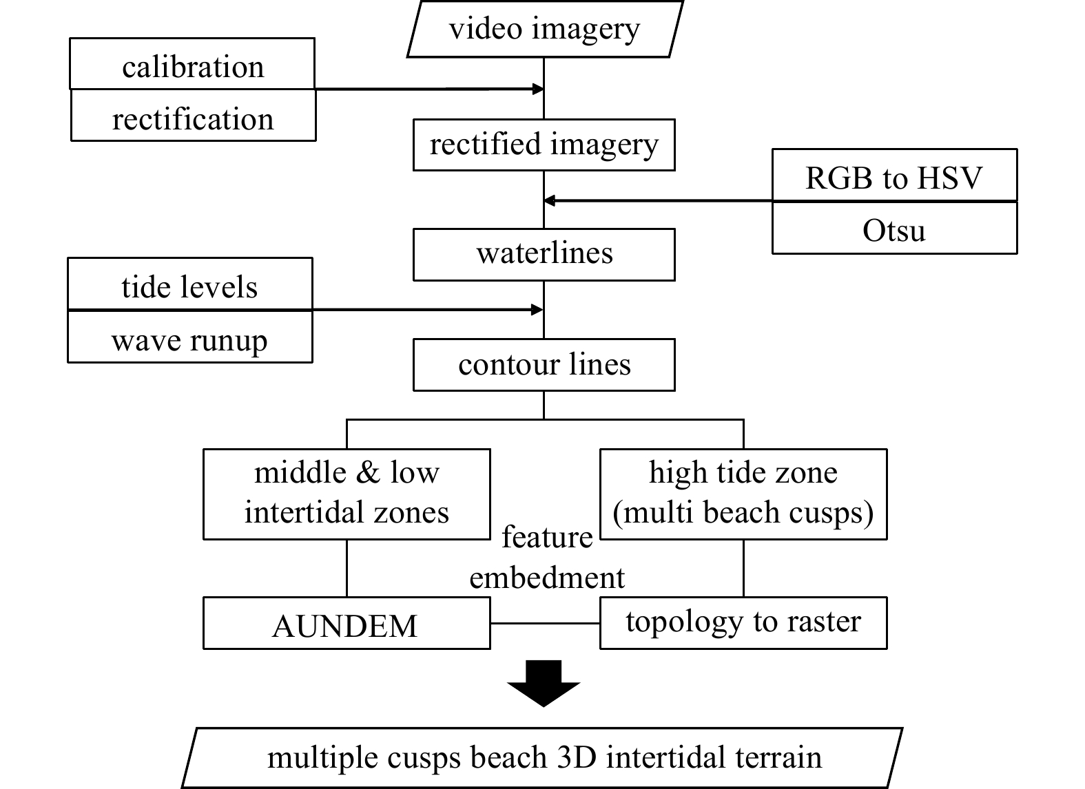
By combining Geographic Information System (GIS) techniques with various video imagery processing algorithms, a specialized methodology was proposed for reconstructing intertidal DEMs for beaches with multiple cusps (Fig. 2). Based on the object-oriented idea, we introduced feature embedding for precision processing to the beach cusp system DEM and selected more suitable waterline extraction and terrain interpolation algorithms after extensive testing.
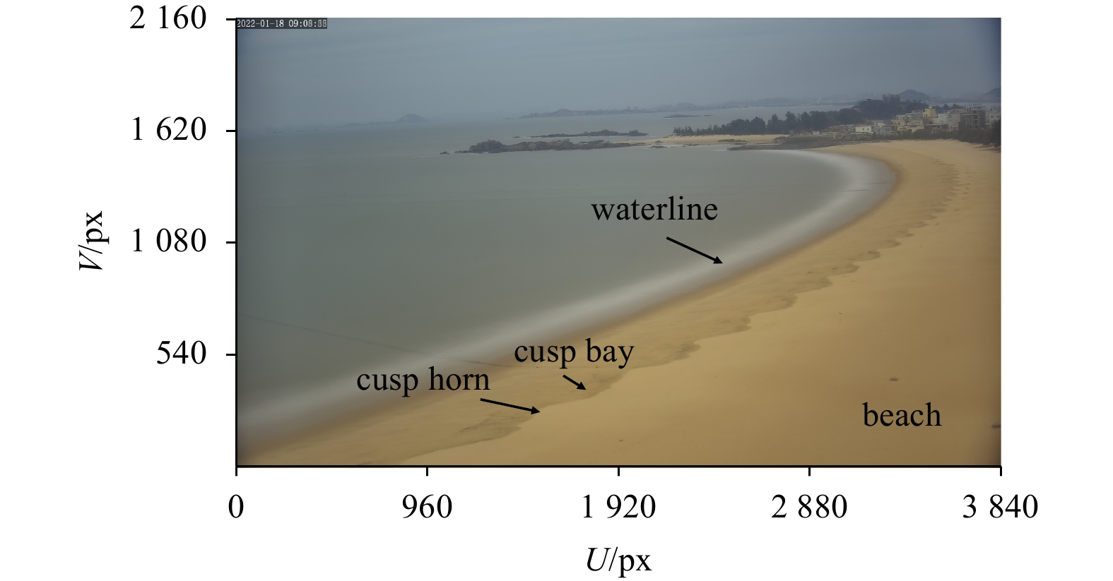
The VMS was set to acquire snap imagery sequences at a frequency of 2 Hz for the first ten minutes (1 200 frames/group) of each hour during the daytime and with a pixel resolution of 3840×2 160. A MATLAB script was used to produce time-exposed (Timex) imagery and time series of pixel intensity values (Timestack) corresponding to each group of snap imagery sequences (Holman and Stanley, 2007). The Timex imagery of the western part of the beach (Fig. 3) shows the spreading characteristics of the BCS, where the temporally smoothed waterline can be used to characterize the water level at that time in the imagery.
Figure
3.
Timex imagery example shot by C4 (U, V).
For quantitative extraction of nearshore information from the VMS, coordinate rectification from the image coordinate system (U, V) to the Cartesian world coordinate system (X, Y, Z) is performed (Holland et al., 1997). For this purpose, calibration (Zhang, 1999) must be carried out to obtain the internal parameters (the intrinsic physical parameters of the cameras) and the external parameters (the geographic position of the cameras and the Euler angles). A total of 14 free parameters need to be determined, and coordinate rectification from (U, V) to (X, Y, Z) was established employing the “common line equation” model (Holland et al., 1997). However, camera parameters are constantly subjected to subtle changes due to disturbances in the external environment that propagate and continue to accumulate during the coordinate rectification process (Sánchez-García et al., 2017). For this reason, we use a new and simplified model proposed by Simarro et al. (2020), which reduces the number of free parameters to 8 by making reasonable approximations. This makes the inversion of the model equations more explicit and allows for automated camera calibration through the application of feature detection and matching algorithms.
For a given point x = (x, y, z) in the world coordinate system, its corresponding distorted coordinates (c, r) in the image coordinate system can be expressed as
where k is the radial distortion factor; s is the pixel size (assumed to be square); (oc, or) are the coordinates of the principal imagery point (assumed to be the center of the imagery); and d2 = u2 + v2, and (u, v) are the undistorted coordinates,
where xc= (xc, yc, zc) are the positions of the camera in the world coordinate system and M = (m1, m2, m3) are the parameters in the orientation matrix calculated through Euler angles (α, τ, θ),
where α is the camera’s azimuth, τ is the pitch, and θ is the lateral tilt.
3.3
Waterline extraction from Timex imagery
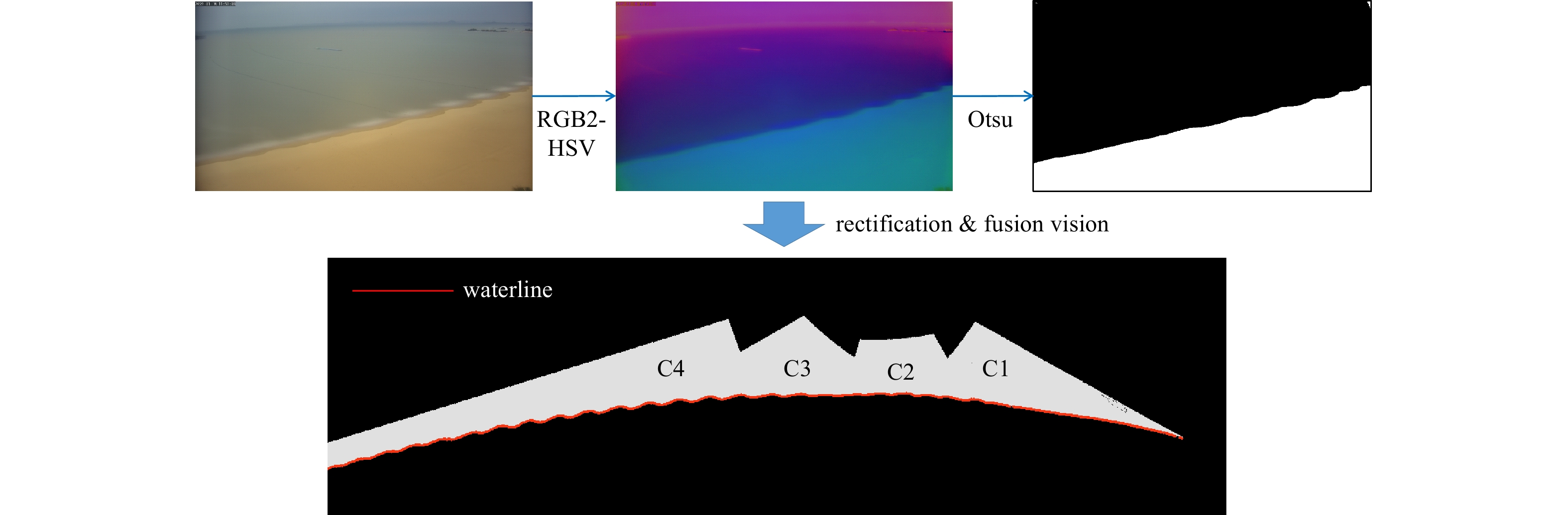
Timex imagery smooths out the high-frequency processes in the swash zone, which results in a less pronounced water‒land edge effect and makes traditional edge detection algorithms less efficient and less accurate in terms of identifying waterlines (Osorio et al., 2012). Aarninkhof et al. (2003) proposed applying HSV (Hue, Saturation, Value) color space in contrast to RGB color space (abbreviated as RGB2HSV algorithm) to enhance the intensity contrast between wet and dry pixels. Moreover, the three components of the HSV model have higher independence. We use the maximum interclass variance algorithm (Otsu) (Otsu, 1979) for the saturation component, which has the best convexity of the waterline. Thus, the optimal threshold is automatically determined, and binarized segmentation is performed. The test results (Fig. 4) show that the combination of the RGB2HSV and Otsu algorithms can improve the efficiency and accuracy of waterline extraction while facilitating a more detailed portrayal of the morphological features of the BCS.
The waterlines extracted from the Timex imagery represent the horizontal location of wave runup at that time. Water level data are used to assign elevations to the waterlines at different tidal phases to obtain intertidal elevation contours. Aarninkhof et al. (2003) gave a “normalized” formula for the waterline elevation,
$$ {z}_{sl}={z}_{o}+{\eta }_{sl}+{z}_{s} ,$$
(4)
where zsl is the waterline elevation, zo includes the astronomical tidal and meteorological nearshore water elevations, ηsl is the wave setup, and zs is the oscillation of the waterline elevation due to wave runup and rundown.
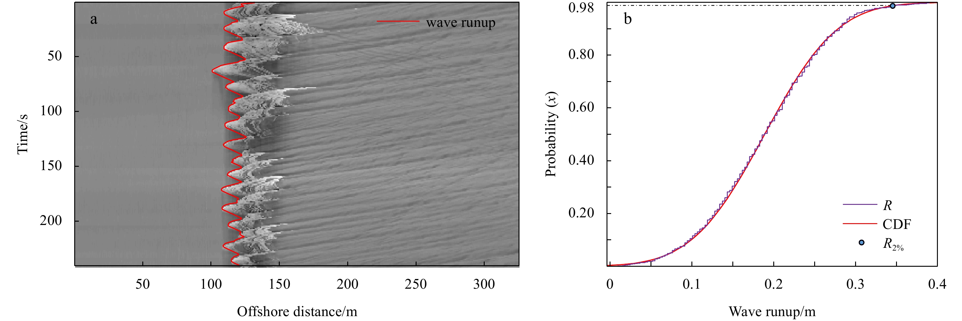
The terms zo and ηsl in Eq. (4) are generally obtained from in situ observations or through local tide gauge stations. While wave runup, as a high-frequency dynamic process, is more difficult to measure in situ (Aarninkhof et al., 2003). Holland et al. (1995) proposed the use of VMSs to collect cross-shore pixel intensity time series to digitally extract the wave runup dynamics based on the sharp pixel brightness contrast between the whitecaps and the background beach (Palmsten and Brodie, 2022). Compared with the measured wave runup threshold R2%(Atkinson et al., 2017), the average positioning accuracy of the algorithm was controlled within 20%, suggesting that it is an effective method for wave runup measurements (da Silva et al., 2020) (Fig. 5).
Figure
5.
Digital extraction of wave runup height at Xisha Gulf beach (a); R2% identification from normal cumulative distribution function (CDF) (b).
3.5
Terrain interpolation and feature embedment within the DEM
The above algorithm was used to obtain intertidal elevation contours with a temporal resolution of 1 h. Multiple contours for one tidal cycle were imported into ArcMap 10.5, and the ANUDEM interpolation algorithm (Hutchinson, 1989) was then used. In ArcGIS, ANUDEM has been integrated into an efficient, semiautomated topographic toolbox consisting of four steps: interpolation, data smoothing, terrain enforcement, and the application of locally adaptive strategies. The algorithm has the advantage that by imposing constraints on the interpolation process, the geomorphological features associated with erosion driven by flowing water can be better represented, thus making it suitable for topographic interpolation within tidal flats (Zhang et al., 2022).
Terrain interpolation can effectively depict the overall topographic trends in the intertidal area. However, due to the relatively complex geomorphic structure of the BCS, it is easily smoothed out during this process. Herein, we propose to enhance the microgeomorphologic details that represent the BCS in the high tide zone by embedding the features into the DEM (Wang et al., 2009) with the following three steps: (1) increase the temporal resolution of the Timex imagery over the high tide zone from 1 h to 0.5 h; (2) precisely process the morphological structure of the beach cusps through visual interpretation and GIS editing and assist the RGB2HSV and Otsu algorithm to ensure more accurate contour extraction; and (3) the triangulated irregular network of the high tidal zone is transformed into a higher spatial resolution (0.30 m) DEM using the topology-to-raster tool and is then mosaiced with the initial intertidal DEM, thus completing the reconstruction of the 3D terrain of the entire intertidal area while preserving the multiple beach cusps.
4.
Field experiment, validation, and analysis
4.1
Field survey
In January 2022, a field experiment was carried out at Xisha Gulf beach. Six cross-shore profiles were laid out and measured at 200 m intervals along the shoreline. In addition, the elevations of more than six hundred sampling points were calculated from east to west in the high tide zone (the region where the BCS developed). The instrument used for the measurements was a Stonex-S9II RTK-GPS, and the horizontal and vertical errors were ±5 mm+1×10⁻⁶ RMS and ±10 mm+1×10⁻⁶ RMS, respectively. All surveys are based on the same geographical reference system, World Geodetic System 1984 (WGS-84), and are projected to the planar coordinate system, Universal Transverse Mercator (UTM) Zone 50 N.
Moreover, an RBR solo3D wave16 wave gauge was deployed at the subtidal zone of Xisha Gulf beach with a sampling interval of 10 min and a frequency of 4 Hz to obtain water levels and nearshore wave parameters. During the field experiment (2022-01-17 06:00 to 2022-01-19 04:20), Xisha Gulf beach experienced four tidal cycles with an average tidal difference of approximately 4.500 m; the significant wave height ranged from 0.139 m to 0.338 m, with a mean value of 0.207 m (Fig. 6). The overall macrotidal conditions and low-energy environment imply an extensive intertidal zone where wave processes have little effect on the water level, which are conditions beneficial for VMS-based DEM reconstruction.
Figure
6.
Water level and significant wave height at Xisha Gulf beach during the experimental period (2022-01-17 06:00 to 2022-01-19 04:20).
Based on the methodology described in Section 3, combined with the field water level observation data, the DEM of the intertidal zone of Xisha Gulf beach was reconstructed, which included the embedded BCS (Fig. 7). The final intertidal DEM has a visually crisp and smooth effect, which allows the geomorphological features along the intertidal beach produced by continuous hydrodynamic scouring to be fully represented. In particular, the unique microgeomorphology of the horn-bay-horn pattern of the BCS is clearly outlined in the high tide zone of the DEM with embedded BCS features.
Figure
7.
Digital elevation model reconstruction effect of the intertidal zone at Xisha Gulf beach, including validation profiles and instrument layout (WGS-84 UTM 50 N zone). BCS: beach cusp system; VMS: video monitoring system.
The vertical accuracy of the intertidal DEM derived by video imagery was evaluated using the RTK-GPS measured profiles. Table 1 shows the comparison between the six profiles measured by the RTK and the measurements extracted from the VMS. The average vertical error is expressed by RMSE,
Table
1.
Average slope of the swash zone (tan β), mean vertical error (Δmean), minimum vertical error (Δmin), and maximum vertical error (Δmax) of the verified profiles
where Δmean is the average vertical error expressed in terms of RMSE, Xrtk is the RTK-GPS measured reference values, Xvms is the VMS measured values of the corresponding points, and n is the total number of the corresponding points.
The corresponding points in profiles P1–P5 show evidence of both underestimation and overestimation, with average vertical errors below 5% of the tidal difference in the study area, which is comparable to the RTK-GPS positioning accuracy in magnitude. However, the vertical accuracy of P6, which is farther away from the VMS, is relatively poor (vertical RMSE = 0.264 m), and the relative error indicates an overall overestimation with a maximum of 0.423 m.
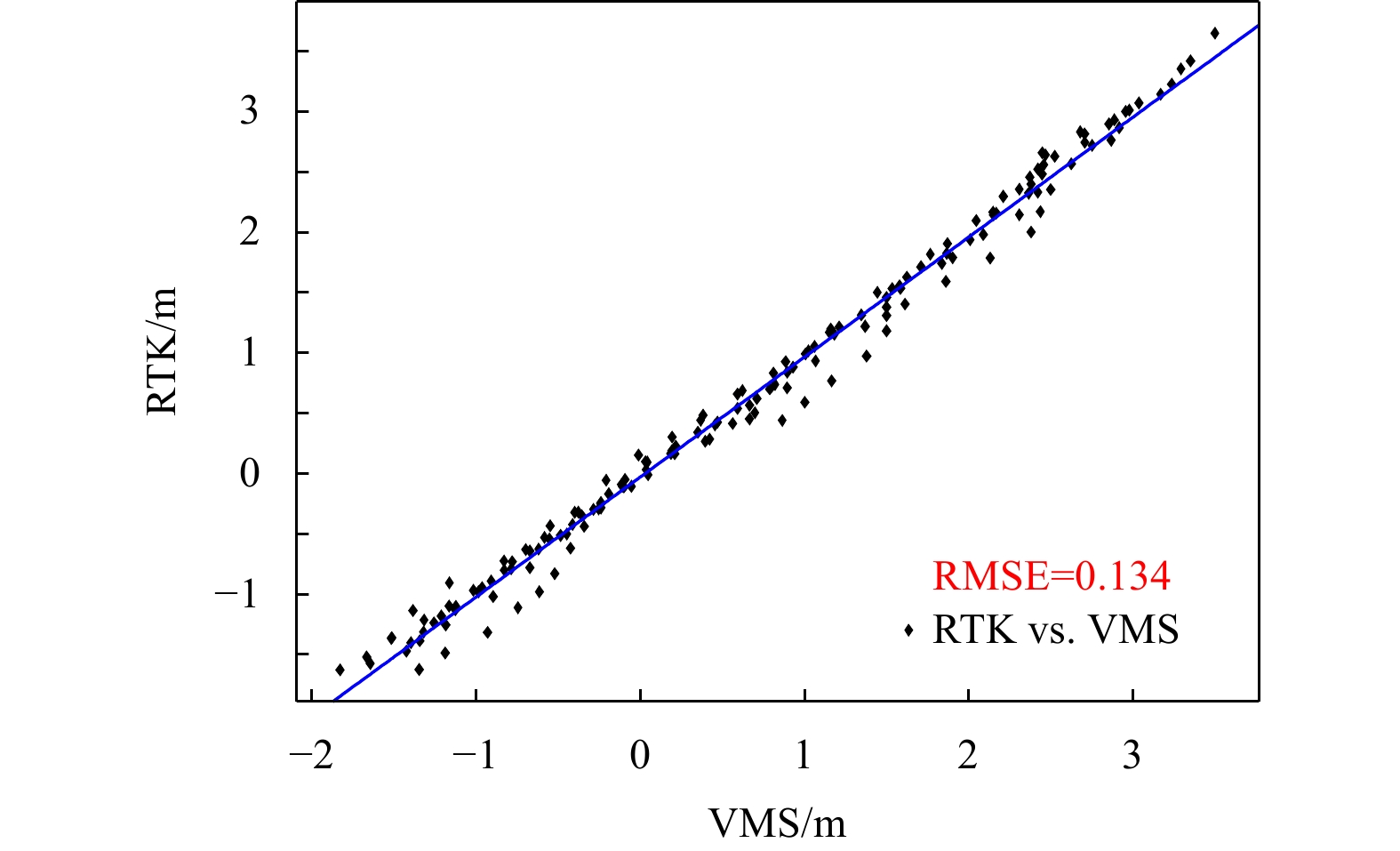
There is a good correlation between the VMS-derived values and the corresponding points from the RTK-GPS measurements for all six profiles (Fig. 8), with an R2 value reaching 0.991, a sum of squared errors (SSE) of 2.888 m, and an RMSE of 0.134 m. Taking the presence of systematic errors and wave runup (R2%) calculation errors into account, the average vertical positioning accuracy of the intertidal DEM constructed in this study is within 0.150 m.
Figure
8.
Correlation fit of the corresponding points on all six profiles. VMS: video monitoring system; RTK: Real-time kinematic.
4.3.2
Profile accuracy evaluation and error analysis
The overall accuracy of the intertidal DEM was verified by the measured profiles, and the average vertical accuracy of the intertidal profiles derived from the video imagery was within 0.150 m, which is comparable to the accuracy obtained by combining LIDAR-video measurements as reported by Andriolo et al. (2018). This indicates that the reconstruction results provide a good indication of the morphological evolution of the intertidal zone over long time scales. This method allows for some assessment of short-term morphological changes in terrain and microrelief. The high-frequency sampling capability and reliability of the VMS also allow for the observation of short-term and abrupt morphological changes in the intertidal zone, such as those caused by anomalous events (e.g., storm surges, cold winter waves, and human activities).
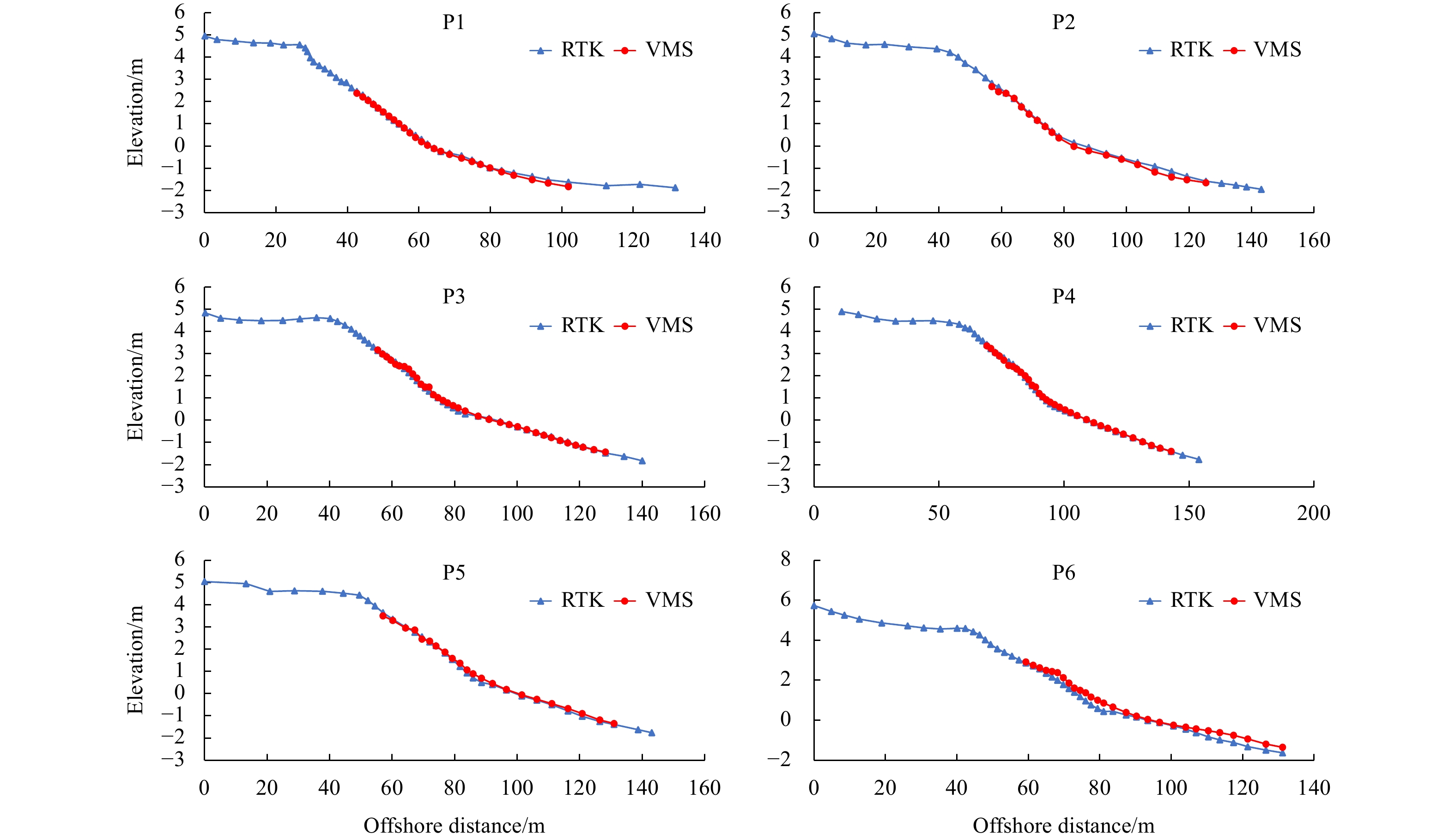
Despite careful consideration of the elements that impact water level elevation, the intertidal DEM profile validation results obtained in this study still have some errors and show significant spatial variability. As shown in Fig. 9, profiles P3 and P4 are located in the central area of the observation field of view. These are relatively closest to the VMS (<200 m) and show the highest quality results (vertical accuracy within 0.100 m). Profiles P1 and P2 are located on the east side of the beach, and the results underestimated the low tide zones. P6 is located in the western part of the beach, more than 500 m away from the VMS, and was determined to have the greatest overestimation.Holman and Stanley, (2007) observed that this is because the increase in the observation distance leads to a reduction in spatial resolution. Therefore, the same image coordinate rectification accuracy (controlled to within 10 pixels in this study) can lead to diverse horizontal offsets when extracting the waterlines that correspond to different tide levels. On the other hand, an accurate estimation of the Euler angles will guarantee that the accuracy of the video imagery when performing coordinate conversion is maintained (Holland et al., 1995). When the camera is mounted on the side of the beach, the inclined attitude is not conducive to properly estimating the Euler angles. Therefore, when considering where to set up the VMS, a higher elevation position in the middle of the beach with the best observation view is ideal.
Figure
9.
Comparison of video-derived intertidal profiles with RTK-GPS-measured profiles. RTK: Real-time kinematic; VMS: video monitoring system.
4.4
Verification and analysis of the BCS terrain model accuracy
4.4.1
Multiple beach cusps identification
The number and spacing of beach cusps were measured using the waterline corresponding to the high tide level as a proxy. The results show that a total of 38 individual beach cusps with an average interval of approximately 20 m were identified within the combined field of view of the four cameras, of which five cusps were distributed independently within the field of view of C2, and the remaining 33 were distributed continuously within the field of view of C3 and C4. The counts and spacing measurements are in general agreement with the results of the field observations.
4.4.2
Validation and comparative analysis of the BCS DEM accuracy
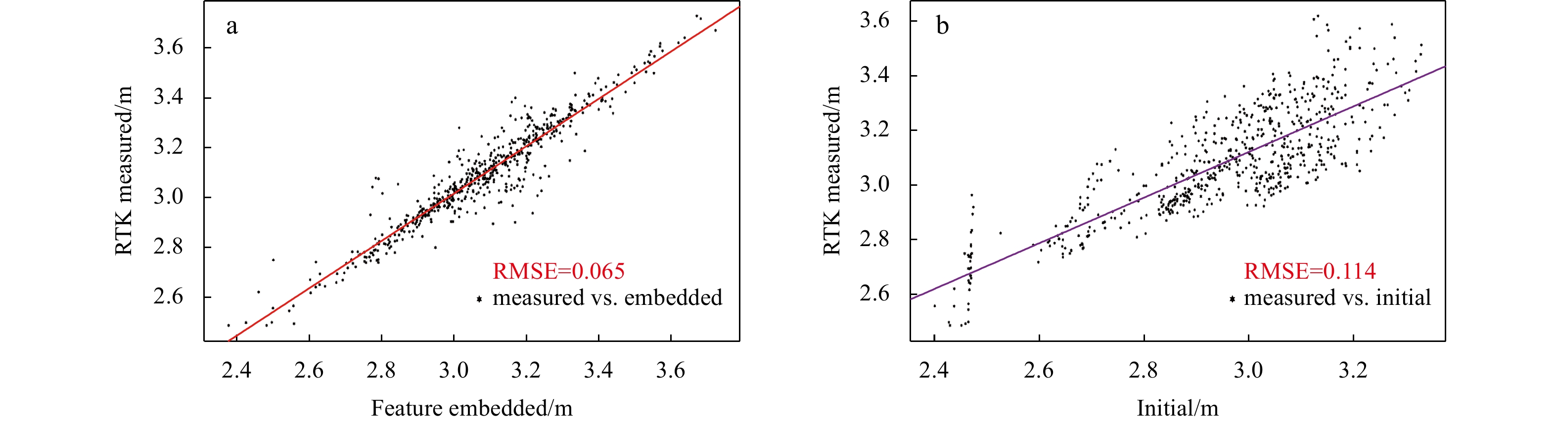
The RMSE obtained from the profile validation reflects the overall accuracy of the intertidal DEM from the land to sea, but the results were relatively poor within the different subdivisions of the intertidal zone. A targeted assessment of the BCS was carried out. Six hundred sampling points were taken throughout the horns and bays of all the beach cusps at Xisha Gulf beach, which were then correlated with the values extracted from the corresponding points in the DEM (Fig. 10).
Figure
10.
Comparison of the feature embedment beach cusp system (BCS) digital elevation mode (DEM) and the corresponding RTK-GPS measured points (a); comparison of the initial DEM and the corresponding RTK-GPS measured points (b). RTK: Real-time kinematic.
The results show that the DEM with the embedded features corresponds to the direct surface measurements with a higher R2 value (0.903 vs. 0.674), lower SSE (2.479 m vs. 8.115 m), and smaller RMSE (0.065 m vs. 0.114 m) than the initial DEM. Notably, the values extracted from the initial DEM show a relatively significant underestimation at the BCS location in terms of the trend line. In contrast, after precision processing and feature embedment, the values extracted from the DEM more closely matched the measured values. It can be stated that the DEM with the embedded BCS features (i.e., BCS DEM) is a significant improvement compared to the initial DEM in terms of goodness of fit and vertical accuracy.
4.4.3
BCS embedded DEM effect and discussion
Embedding features is an effective method of enhancing DEM detail and has been successfully applied to nearshore sandy intertidal landscapes (Zhou et al., 2021), tidal flats, and trenches (Zhang et al., 2022). In this study, the method was used to enhance the details of the unique structural features of BCSs, and the mean vertical accuracy was further improved to within 0.100 m. It can be stated that the BCS DEM obtained in this study is satisfactory in terms of both visual effect and accuracy.
Fully exploiting the sustained observational power of VMSs will have a substantial and positive impact on the study of BCS formation and evolutionary mechanisms. In the USA (van Gaalen et al., 2011), Australia (Montes et al., 2018), and European countries (Almar et al., 2008; Vousdoukas, 2012), some studies have applied video monitoring technology to assess the dynamic geomorphological evolution of BCSs. Furthermore, it is particularly evident that relying on long time series imagery is beneficial to the study of the seasonal evolution pattern of beach cusps. VMS technology was adopted only recently in China, and the details of its users are currently being refined. Tian et al. (2020) reported on the development of beach cusps observed by video imagery as a response to typhoons at Wendeng South beach, Shandong Province. Because of the lack of methods for quantifying 3D topographic changes, the evolutionary mechanisms of beach cusps were not explored in depth. This study presents a means to obtain a BCS DEM with high resolution and high vertical accuracy, which will provide technical support to expand the study of beach cusp formation and evolution.
Comparison with other means of beach terrain observation. Labor-intensive RTK-GPS technology can assure the highest accuracy, but the relatively cumbersome operation and high logistical cost make it difficult to support a high frequency of observation (Lopes et al., 2013). The rapidly developing unmanned aerial vehicle (UAV) technology, coupled with RTK or lidar, is also an effective way to measure beach terrain and microrelief, yet the current research stage still relies on manual deployment, manipulation, and retrieval each time UAV operations are conducted (Pitman et al., 2019; Nuyts et al., 2020). Therefore, the automated, high-frequency information acquisition capability of VMSs determines their irreplaceable role in the field of beach research. It should be particularly noted that the formation mechanism of the beach cusp is somehow associated with storm extremes (Tian et al., 2020), and VMS has the ability to operate stably in all weather, which is not available by RTK, UAV, and other means.
Due to the limitations of VMS performance, the BCS DEM constructed in this study still suffers from specific vertical errors and detail problems, presumably related to the smoothing effect of the Timex imagery on the swash process. The function is not effective in smoothing the waterlines while preserving the microrelief. Constructing the DEM of a specific target beach cusp based on timelapse snap imagery and considering only individual wave runup events may be a more effective solution. Nevertheless, given the random and transient nature of the wave runup process, higher demands are placed on the frequency and accuracy of water level elevation measurements. Herein, coupling video monitoring with automated water level measurement techniques, such as shore-based radar, is advocated to establish a three-dimensional observation system of coastal dynamic and geomorphic processes to continuously monitor the formation and evolution of microgeomorphologic features in real time.
5.
Conclusions
This study proposes a methodology for developing DEMs in the intertidal zone along beaches with multiple cusps. Using video imagery collected over one tidal cycle, the DEM is constructed based on the waterline method. The detailed representation of the BCS is enhanced by embedding features within the DEM. A high degree of vertical accuracy and a clear visual result were obtained, as verified by data collected in situ.
(1) Continuous monitoring by the VMS fully considers the hydrodynamic processes, such as tides and wave runup, that cause oscillations along the waterlines. This allows for a finer characterization of the terrain and microrelief by providing a higher spatial and temporal resolution. By coupling the ANUDEM algorithm with the DEM that contains the embedded features, the three-dimensional terrain of the intertidal zone along a beach with multiple cusps is constructed. This allows for a better representation of the horn-bay-horn interphase distribution pattern of the BCS.
(2) The video-derived DEM was evaluated using RTK-GPS data and had an average vertical accuracy along the measured profiles that was better than 0.150 m. The accuracy can effectively characterize the erosion-accretion patterns of intertidal terrain at different spatial scales. The embedded BCS DEM had an average vertical error within 0.100 m and was significantly more accurate than the initial DEM. Therefore, the BCS DEM can be used to investigate the formation and evolutionary mechanisms of the BCS and its association with hydrodynamic forcing.
(3) The intertidal DEM provided by the VMS shows regional variability. It is fairly intuitive that the vertical accuracy of the video-derived elevations was negatively correlated with the distance of the camera. Embedding the BCS features within the DEM offers a significant improvement in positioning accuracy but still fails to retain the full morphological detail due to the smoothing of the swash process by the Timex imagery. By coupling the methods discussed here with high-frequency water level observation techniques, the study of nearshore topographic evolution by VMS will be further improved.
Acknowledgements:
The authors are grateful to Xisha Gulf holiday hotel for providing the VMS construction site, as well as Haitao Xu, Ronghui Wang, Xu Chen, Yazhuang Zhao (Third Institute of Oceanography, Ministry of Natural Resources) and Jinxin Zhu for their assistance in the field work. We also thank the two anonymous reviewers for their insightful comments.
Aarninkhof S G J, Turner I L, Dronkers T D T, et al. 2003. A video-based technique for mapping intertidal beach bathymetry. Coastal Engineering, 49(4): 275–289. doi: 10.1016/S0378-3839(03)00064-4
Alexander P S, Holman R A. 2004. Quantification of nearshore morphology based on video imaging. Marine Geology, 208(1): 101–111. doi: 10.1016/j.margeo.2004.04.017
Ali S, Darsan J, Wilson M. 2017. Cusp morphodynamics in a micro-tidal exposed beach. Journal of Coastal Conservation, 21(6): 777–788. doi: 10.1007/s11852-017-0536-2
Almar R, Blenkinsopp C, Almeida L P, et al. 2019. Intertidal beach profile estimation from reflected wave measurements. Coastal Engineering, 151: 58–63. doi: 10.1016/j.coastaleng.2019.05.001
Almar R, Coco G, Bryan K R, et al. 2008. Video observations of beach cusp morphodynamics. Marine Geology, 254(3–4): 216–223
Andriolo U, Almeida L P, Almar R. 2018. Coupling terrestrial LiDAR and video imagery to perform 3D intertidal beach topography. Coastal Engineering, 140: 232–239. doi: 10.1016/j.coastaleng.2018.07.009
Atkinson A L, Power H E, Moura T, et al. 2017. Assessment of runup predictions by empirical models on non-truncated beaches on the south-east Australian coast. Coastal Engineering, 119: 15–31. doi: 10.1016/j.coastaleng.2016.10.001
Bagot P, Huybrechts N, Sergent P. 2021. Satellite-derived topography and morphological evolution around authie macrotidal estuary (France). Journal of Marine Science and Engineering, 9(12): 1354. doi: 10.3390/jmse9121354
Cai Feng, Cao Chao, Qi Hongshuai, et al. 2022. Rapid migration of mainland China’s coastal erosion vulnerability due to anthropogenic changes. Journal of Environmental Management, 319: 115632. doi: 10.1016/j.jenvman.2022.115632
Cai Feng, Cao Huimei, Su Xianze, et al. 2007. Analysis on morphodynamics of sandy beaches in South China. Journal of Coastal Research, 23(1): 236–246
Ciriano Y, Coco G, Bryan K R, et al. 2005. Field observations of swash zone infragravity motions and beach cusp evolution. Journal of Geophysical Research: Oceans, 110(C2): C02018
Coco G, Huntley D A, O’Hare T J. 2000. Investigation of a self-organization model for beach cusp formation and development. Journal of Geophysical Research: Oceans, 105(C9): 21991–22002. doi: 10.1029/2000JC900095
Coco G, O’Hare T J, Huntley D A. 1999. Beach cusps: a comparison of data and theories for their formation. Journal of Coastal Research, 15(3): 741–749
da Silva P G, Coco G, Garnier R, et al. 2020. On the prediction of runup, setup and swash on beaches. Earth-Science Reviews, 204: 103148. doi: 10.1016/j.earscirev.2020.103148
Davies J L. 1964. A morphogenic approach to world shorelines. Zeitschrift für Geomorphologie, 8(5): 127–142
Guest T B, Hay A E. 2019. Timescales of beach cusp evolution on a steep, megatidal, mixed sand-gravel beach. Marine Geology, 416: 105984. doi: 10.1016/j.margeo.2019.105984
Holland K T, Holman R A, Lippmann T C, et al. 1997. Practical use of video imagery in nearshore oceanographic field studies. IEEE Journal of Oceanic Engineering, 22(1): 81–92. doi: 10.1109/48.557542
Holland K T, Raubenheimer B, Guza R T, et al. 1995. Runup kinematics on a natural beach. Journal of Geophysical Research: Oceans, 100(C3): 4985–4993. doi: 10.1029/94JC02664
Holman R A, Stanley J. 2007. The history and technical capabilities of Argus. Coastal Engineering, 54(6–7): 477–491
Hutchinson M F. 1989. A new procedure for gridding elevation and stream line data with automatic removal of spurious pits. Journal of Hydrology, 106(3–4): 211–232
Liu Yongxue, Li Manchun, Zhou Minxi, et al. 2013. Quantitative analysis of the waterline method for topographical mapping of tidal flats: a case study in the dongsha sandbank, China. Remote Sensing, 5(11): 6138–6158. doi: 10.3390/rs5116138
Lopes V, Baptista P, Pais-Barbosa J, et al. 2013. DGPS based methods to obtain beach cusp dimensions. Journal of Coastal Research, 65(sp1): 541–546
Mason D C, Davenport I J, Robinson G J H, et al. 1995. Construction of an inter-tidal digital elevation model by the ‘Water-Line’ Method. Geophysical Research Letters, 22(23): 3187–3190. doi: 10.1029/95GL03168
Montes J, Simarro G, Benavente J, et al. 2018. Morphodynamics assessment by means of mesoforms and video-monitoring in a dissipative beach. Geosciences, 8(12): 448. doi: 10.3390/geosciences8120448
Nuyts S, Li Zili, Hickey K, et al. 2021. Field observations of a multilevel beach cusp system and their swash zone dynamics. Geosciences, 11(4): 148. doi: 10.3390/geosciences11040148
Nuyts S, Murphy J, Li Zili, et al. 2020. A methodology to assess the morphological change of a multilevel beach cusp system and their hydrodynamics: case study of Long Strand, Ireland. Journal of Coastal Research, 95(S1): 593–598
Osorio A F, Medina R, Gonzalez M. 2012. An algorithm for the measurement of shoreline and intertidal beach profiles using video imagery: PSDM. Computers & Geosciences, 46: 196–207
Otsu N. 1979. A threshold selection method from gray-level histograms. IEEE Transactions on Systems, Man, and Cybernetics, 9(1): 62–66
Palmsten M L, Brodie K L. 2022. The coastal imaging research network (CIRN). Remote Sensing, 14(3): 453. doi: 10.3390/rs14030453
Pitman S J, Hart D E, Katurji M H. 2019. Application of UAV techniques to expand beach research possibilities: a case study of coarse clastic beach cusps. Continental Shelf Research, 184: 44–53. doi: 10.1016/j.csr.2019.07.008
Plant N G, Holman R A. 1997. Intertidal beach profile estimation using video images. Marine Geology, 140(1–2): 1–24
Qi Hongshuai, Cai Feng, Lei Gang, et al. 2010. The response of three main beach types to tropical storms in South China. Marine Geology, 275(1–4): 244–254
Salameh E, Frappart F, Almar R, et al. 2019. Monitoring beach topography and nearshore bathymetry using spaceborne remote sensing: a review. Remote Sensing, 11(19): 2212. doi: 10.3390/rs11192212
Sánchez-García E, Balaguer-Beser A, Pardo-Pascual J E. 2017. C-Pro: a coastal projector monitoring system using terrestrial photogrammetry with a geometric horizon constraint. ISPRS Journal of Photogrammetry and Remote Sensing, 128: 255–273. doi: 10.1016/j.isprsjprs.2017.03.023
Simarro G, Calvete D, Souto P, et al. 2020. Camera calibration for coastal monitoring using available snapshot images. Remote Sensing, 12(11): 1840. doi: 10.3390/rs12111840
Soloy A, Turki I, Lecoq N, et al. 2021. A fully automated method for monitoring the intertidal topography using Video Monitoring Systems. Coastal Engineering, 167: 103894. doi: 10.1016/j.coastaleng.2021.103894
Tian Ye, Yin Ping, Jia Yonggang, et al. 2020. Response of beach characteristics to typhoon “Yagi”: evidence from Argus video images and on-site measurement. Marine Geology & Quaternary Geology (in Chinese), 40(5): 201–210
Uunk L, Wijnberg K M, Morelissen R. 2010. Automated mapping of the intertidal beach bathymetry from video images. Coastal Engineering, 57(4): 461–469. doi: 10.1016/j.coastaleng.2009.12.002
van Gaalen J F, Kruse S E, Coco G, et al. 2011. Observations of beach cusp evolution at Melbourne Beach, Florida, USA. Geomorphology, 129(1–2): 131–140
Van Koningsveld M, Davidson M, Huntley D, et al. 2007. A critical review of the CoastView project: recent and future developments in coastal management video systems. Coastal Engineering, 54(6–7): 567–576
Vousdoukas M I. 2012. Erosion/accretion patterns and multiple beach cusp systems on a meso-tidal, steeply-sloping beach. Geomorphology, 141–142: 34–46
Vousdoukas M I, Ferreira P M, Almeida L P, et al. 2011. Performance of intertidal topography video monitoring of a meso-tidal reflective beach in South Portugal. Ocean Dynamics, 61(10): 1521–1540. doi: 10.1007/s10236-011-0440-5
Wang Chun, Tang Guoan, Liu Xuejun, et al. 2009. The model of terrain features preserved in grid DEM. Geomatics and Information Science of Wuhan University (in Chinese), 34(10): 1149–1154
Zhang Zhengyou. 1999. Flexible camera calibration by viewing a plane from unknown orientations. In: Proceedings of the Seventh IEEE International Conference on Computer Vision. Kerkyra: IEEE
Zhang Dong, Zhang Huiming, Zhou Yong, et al. 2022. An evaluation of wind turbine-induced topographic change in the offshore intertidal sandbank using remote sensing-constructed digital elevation model data. Remote Sensing, 14(9): 2255. doi: 10.3390/rs14092255
Zhou Yong, Zhang Dong, Deng Huili, et al. 2021. The enhanced construction method for intertidal terrain of offshore sandbanks by remote sensing. Haiyang Xuebao (in Chinese), 43(12): 133–143
Nan Xu, Lin Wang, Hao Xu, et al. Deriving Accurate Intertidal Topography for Sandy Beaches Using ICESat-2 Data and Sentinel-2 Imagery. Journal of Remote Sensing, 2024, 4 doi:10.34133/remotesensing.0305
Feng Cai, Hang Yin, Hongshuai Qi, Jixiang Zheng, Yuwu Jiang, Zhubin Cao, Yanyu He. Using video imagery to reconstruct the 3D intertidal terrain along a beach with multiple cusps[J]. Acta Oceanologica Sinica, 2023, 42(7): 1-9. doi: 10.1007/s13131-023-2174-x
Feng Cai, Hang Yin, Hongshuai Qi, Jixiang Zheng, Yuwu Jiang, Zhubin Cao, Yanyu He. Using video imagery to reconstruct the 3D intertidal terrain along a beach with multiple cusps[J]. Acta Oceanologica Sinica, 2023, 42(7): 1-9. doi: 10.1007/s13131-023-2174-x
Table
1.
Average slope of the swash zone (tan β), mean vertical error (Δmean), minimum vertical error (Δmin), and maximum vertical error (Δmax) of the verified profiles
Figure 1. Location of Xisha Gulf beach, including validation profiles and instrument layout (a, b); the video monitoring system (VMS) at Xisha Gulf beach (4 cameras set up on the open terrace on the top floor of the Xisha Gulf holiday hotel) (c, d).
Figure 2. Flow chart of the proposed methodology.
Figure 3. Timex imagery example shot by C4 (U, V).
Figure 5. Digital extraction of wave runup height at Xisha Gulf beach (a); R2% identification from normal cumulative distribution function (CDF) (b).
Figure 6. Water level and significant wave height at Xisha Gulf beach during the experimental period (2022-01-17 06:00 to 2022-01-19 04:20).
Figure 7. Digital elevation model reconstruction effect of the intertidal zone at Xisha Gulf beach, including validation profiles and instrument layout (WGS-84 UTM 50 N zone). BCS: beach cusp system; VMS: video monitoring system.
Figure 8. Correlation fit of the corresponding points on all six profiles. VMS: video monitoring system; RTK: Real-time kinematic.
Figure 9. Comparison of video-derived intertidal profiles with RTK-GPS-measured profiles. RTK: Real-time kinematic; VMS: video monitoring system.
Figure 10. Comparison of the feature embedment beach cusp system (BCS) digital elevation mode (DEM) and the corresponding RTK-GPS measured points (a); comparison of the initial DEM and the corresponding RTK-GPS measured points (b). RTK: Real-time kinematic.


 DownLoad:


 DownLoad:


 DownLoad: